Introduction
Fuel cells powered by liquid hydrogen are a promising propulsion technology to reduce environmentally harmful emissions such as
Besides control, transient behavior and degradation the thermal management is one of the key challenges which have to be overcome by engineers to establish fuel cells as a competitive propulsion technology in aviation. In contrast to gas turbines or piston engines, fuel cells release only 10% to 20% of their waste heat by their exhaust flow (Berger, 2009). With the exception of a small system power up to approximately 3 kW, fuel cell stacks must be cooled directly with a cooling fluid (Barbir, 2013). As the efficiency of the fuel cell system is about 50%, approximately the same amount of power the fuel cell provides as electric power has to be released by the thermal management. From a heat exchange perspective, the low operating temperature range of 60 °C to 90 °C of a LT-PEMFC poses an additional challenge. For hot day conditions (
The large amount of waste heat and the small temperature difference result in large heat exchanger surfaces. The additional drag and weight of the heat exchanger is particularly disadvantageous for an aviation application. The challenge of cooling a fuel cell is also apparent in flying testbeds, which are equipped with large cooling air ducts that contain the heat exchangers. To either reduce the necessary heat exchanger surface by increasing the cooling air velocity or to compensate the loss of momentum of the cooling air flow, an additional cooling fan can be installed. However, it is important to note that such a cooling fan requires a significant amount of electric power, which must also be provided by the fuel cell.
Early publications on the design of fuel cell systems for aircraft propulsion have often simplified the thermal management to a function of the fuel cell power in terms of mass and power demand (Moffitt et al., 2006; Thirkell et al., 2017; Kadyk et al., 2018, 2019; Nicolay et al., 2021; Palladino et al., 2021). The additional drag due to the heat exchanger frontal area was completely neglected. Recent publications have focused on the detailed design of the thermal management system and evaluated its impact on the overall propulsion system. Kožulović (2020) has designed a heat exchanger for a mid-size airliner based on a counterflow liquid-air heat exchanger with corrugated fins. The heat exchanger is installed within a cowling with a diffusor and nozzle but without an additional fan. His analysis states that the propulsion power requirement increases by 27.3% during cruise phase due to the heat exchanger. The design is most efficient when reducing the air velocity prior to the heat exchanger to 15% of the freestream velocity. A subsequent study by Juschus (2021) is based on this approach. Hintermayr and Kazula (2023) optimized the air duct inlet of a 300 kW fuel cell system in terms of performance and sizing. They also considered an additional cooling fan to compensate the total pressure loss of the inlet section. In their studies, the fan had a power of about 20% to 95% of the fuel cell power, showing a strong dependency on the total pressure ratios of the inlet section and the heat exchanger. Hartmann et al. (2022) designed a thermal management for a fuel cell system that uses the liquid hydrogen as a heat sink. The remaining waste heat has to be dissipated by a heat exchanger with a fan. The used design approach does not rely on physics-based calculations to size the thermal management. Instead, scaling factors for the mass and the power demand by evaluating existing studies on aircraft heat exchangers have been used. Kellermann et al. (2021) designed a thermal management system using ram air and an additional cooling fan. The authors demonstrated that a fan can reduce the fuel burn for a turboelectric propulsion system and thereby increase its overall efficiency. Especially under hot conditions, the fan is beneficial in terms of reducing mass, drag, and fuel consumption. An architecture without a fan would need to be significantly larger to meet the same requirements. Eissele et al. (2023) used the results of Kellermann et al. (2021) to develop a scaling factor for the heat exchanger drag. They applied this scaling factor to a fuel cell propulsion system as part of an overall aircraft design but neglected the additional power demand.
Overall, the thermal management causes additional drag, weight and electric power demand in a relevant order of magnitude. The performance of the propulsion system is directly affected by the design of the heat exchanger and the cooling fan. Therefore, the thermal management design cannot be covered by simple scaling factors in the performance calculation of a fuel cell propulsion system but must be integrated into the design process.
This paper is structured as follows: The methodology for calculating the performance is presented first. This includes the definition of the cycle processes, the development of the applied component models and the design algorithm to solve the design problem. In the next section we conduct a design exploration study for typical design variables to demonstrate the benefits of the novel performance calculation approach. Finally, the results of the study for a reference propulsion system are presented and discussed.
Methodology
First, we give a brief introduction to the propulsion system under study. Then, we examine the cycle process of the propeller and the thermal management. By combining the energy conversion and the cycle processes, we derive general equations for the performance calculation of a fuel cell propulsion system. Similar to conventional propulsion systems we define thrust, efficiency and specific fuel consumption. To calculate the thermodynamic processes between the separate stations as well as the energy conversion of the fuel cell powertrain we develop component models. The methodology section concludes with a description of the iterative design calculation process that uses the component models to solve the cycle processes.
Performance calculation
This section describes the performance calculation of the fuel cell propulsion system. We first examine the energy conversion in the powertrain system from the hydrogen tank to the shaft power of the propeller and the resulting conversion losses. Next, we analyze the propeller and the thermal management by interpreting them as two independent cycle processes. The stations for each process are defined, and the state changes are sketched in the
Fuel cell powertrain
The fuel cell powertrain is shown in Figure 1. A cryogenic tank supplies hydrogen with the power
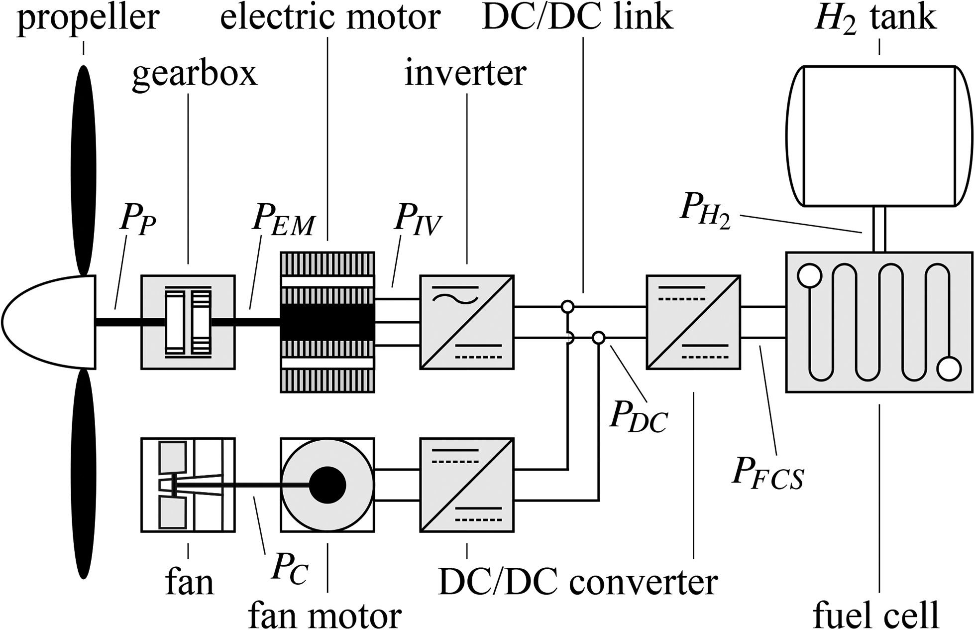
In addition to the powertrain path, the DC bus also supplies power to additional loads. This includes the power required by the cooling air fan, denoted as
During the numerous energy conversions, losses depending on the component efficiencies
Cycle process of the propeller
Figure 2 shows the stations of the propeller cycle process (Figure 2a) and the thermodynamic state changes in the
Figure 2.
Cycle process of the propeller of an aircraft fuel cell propulsion system. (a) Stations and (b) Thermodynamic changes in h , s
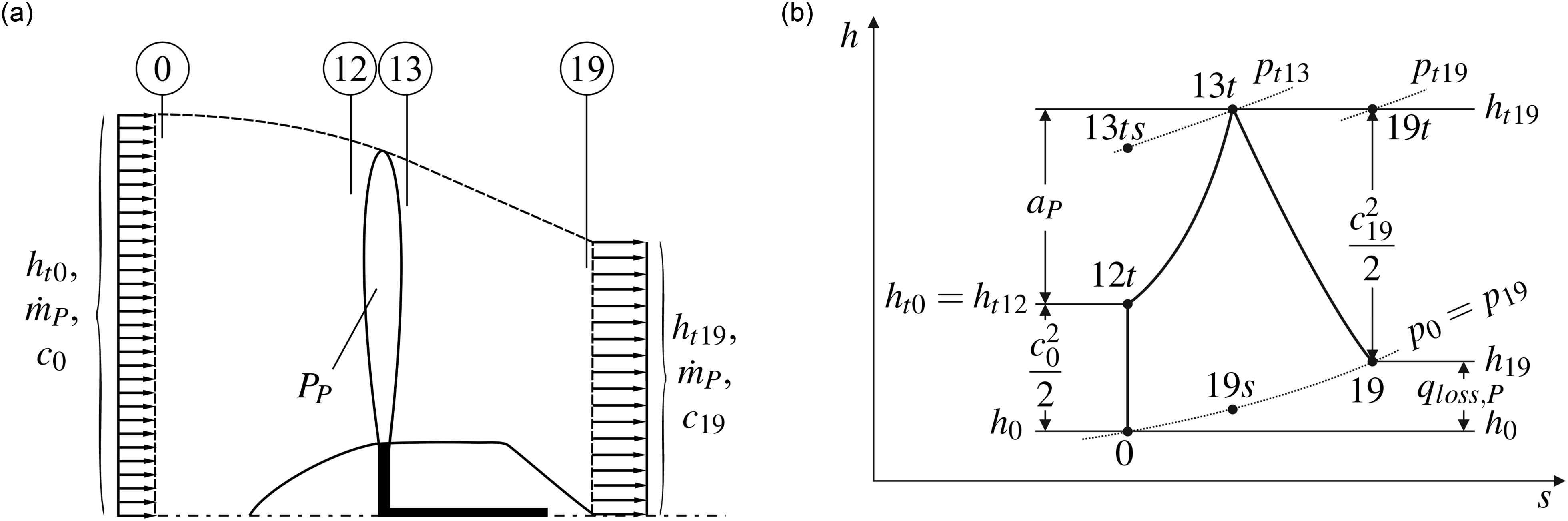
with the propeller mass flow
However, the supplied power is not isentropically converted into a total pressure increase. Therefore, we define the isentropic propeller efficiency
Similarly, the isentropic nozzle efficiency
which leads us to the thermal efficiency of the propeller with Equation 3
As the static pressures upstream and downstream of the propeller are equal
which leads us to the propulsion power
With the equations above the cycle process of the propeller is completely defined.
Cycle process of the thermal management
Figure 3 presents the stations of the thermal management cycle process (Figure 3a) and the thermodynamic state changes in the
Figure 3.
Cycle process of the thermal management of an aircraft fuel cell propulsion system. (a) Stations and (b) Thermodynamic changes in h , s
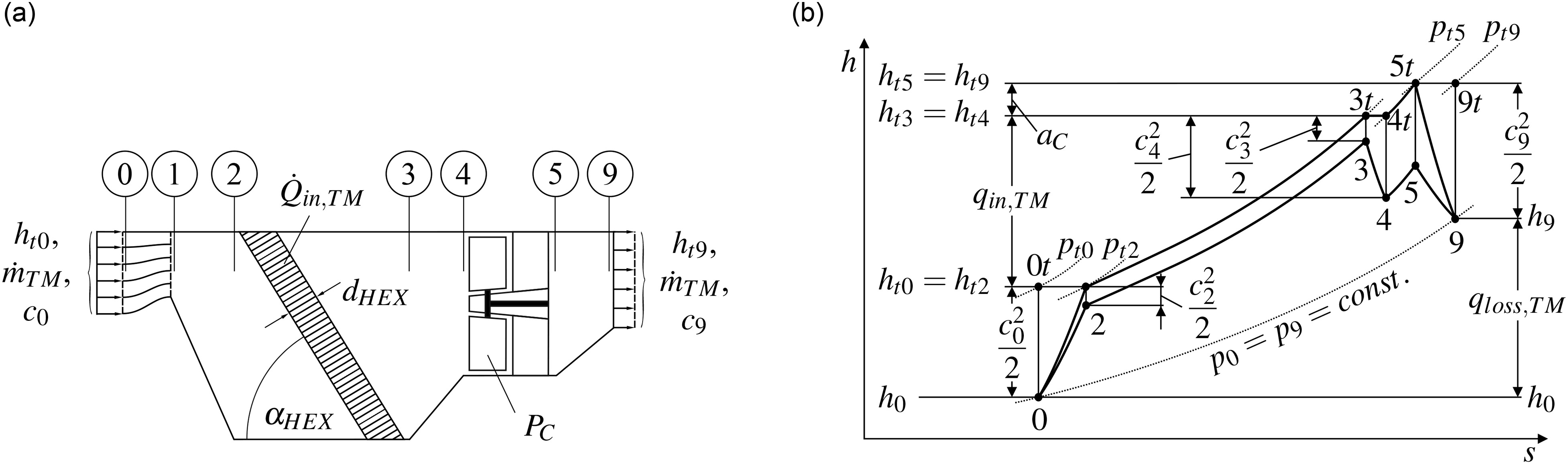
In the heat exchanger from station 2 to 3 the power loss of the energy conversion system Equation 2 is transferred to the cooling air mass flow
Due to inner wall friction as well as expansion and compression of the cooling air, a total pressure loss occurs across the heat exchanger
that is a function of the geometry, fin design, air flow and fluid properties. To decouple the cross sections of the heat exchanger and the cooling fan, a transition duct from station 3 to 4 with the total pressure ratio
is assumed. Between station 4 and 5 a cooling fan with the total pressure ratio
and the isentropic efficiency
Figure 3b demonstrates that the air is perfectly compressed or expanded to ambient pressure (
For this cycle process, we define the power input and output. The usable output power of the cycle process is defined as
As there is a difference in velocity of the air between the inlet and outlet, the cooling air mass flow generates a force
The cowling which covers heat exchanger and cooling fan creates an additional drag
we calculate its propulsion power
Overall propulsion system
The energy conversion processes of the powertrain and propeller, along with the thermal management cycle, have been fully defined. The next step is to aggregate the equations of the three subsystems to calculate the power, thrust, and efficiency of the entire fuel cell propulsion system. The overall usable output power is calculated with Equations 6 and 17
With Equation 21 and the supplied hydrogen power
The total thrust of the fuel cell propulsion system consists of Equations 8 and 19
We also define the specific fuel consumption
with the hydrogen mass flow
with which we calculate the propulsion efficiency
and finally the overall efficiency of propulsion system
Component models
Next, we develop component models which describe the energy conversion and thermodynamic changes of state.
Fuel cell system
As shown in the Figure 1, the fuel cell provides the net electrical power
The fuel cell system consists of multiple stacks, which in turn consist of multiple cells. The operating point of a cell is defined by its current density
which relates the current
we also get the electric power generated by a single cell. With Equation 28 we calculate the number of cells needed
Having defined the operating point and the design of the fuel cell we now calculate the hydrogen consumption of the fuel cell system. The reaction equation of the fuel cell provides the charge number of hydrogen as
and for the fuel cell system with the number of cells from Equation 31
The formula to calculate the hydrogen mass flow is derived in Appendix B. In real operation, more hydrogen is supplied than required for the stoichiometric ratio. In this study, we assume the use of a fuel cell with hydrogen recirculation. Any excess hydrogen that is not consumed is not considered in the fuel calculation as it remains within the system. With Equation 33 and the lower heating value of hydrogen
and the efficiency of the fuel cell system as
The fuel cell system’s total power loss is determined by
A part of the supplied fuel power is released into the environment as waste heat via the exhaust gas flow expressed by the factor
The mass of the fuel cell system
is calculated with the specific power
Heat exchanger
The heat exchanger is illustrated in Figure 3a from station 2 to 3. We assume a plate-fin heat exchanger with offset fins. This is a crossflow heat exchanger with thin fins attached to its plates to increase the heat exchange surface to the passing air. The fins do not run in a longitudinal direction through the entire depth of the heat exchanger. Instead, they end after a certain distance and are offset to the side. This design interrupts the boundary layer formation of the passing cooling air and thus increases the heat transfer. Depending on the heat exchanger’s design, the offsets may be repeated multiple times. This heat exchanger type is appropriate for transferring heat from liquid to gas. It is distinguished by a large heat transfer surface area per unit volume and high heat transfer coefficients at Reynolds numbers ranging from
is defined as the product of the heat exchanger effectiveness
The pressure loss across the heat exchanger defined in Equation 12 is comprised as
consisting of three parts for the inflow into the heat exchanger, the friction in the core and the outflow according to Shah and Sekulić (2003). The core loss accounts for the largest share
significantly influenced by the Fanning friction factor
Cowling
The external drag of the cowling is calculated using a drag coefficient
Thrust is considered positive when the force acts in the direction of flight. Therefore, it is necessary to include a negative sign. Hoerner (1965) gives typical values for drag coefficients of belly-type radiator installations and therefore we define
Since the air always flows perpendicular to
Further propulsion system components
This study does not focus on the powertrain components, such as the electric motor, inverter, and DC/DC converter. Therefore, constant efficiencies and power densities are assumed in the design process. The data utilized in this study are presented in Appendix F. The mass of the gearbox is calculated using a correlation from Brown et al. (2005). A correlation by Chapman et al. (2020) is used for the mass of the cooling fan. The propeller mass was calculated using a correlation from LTH (2022).
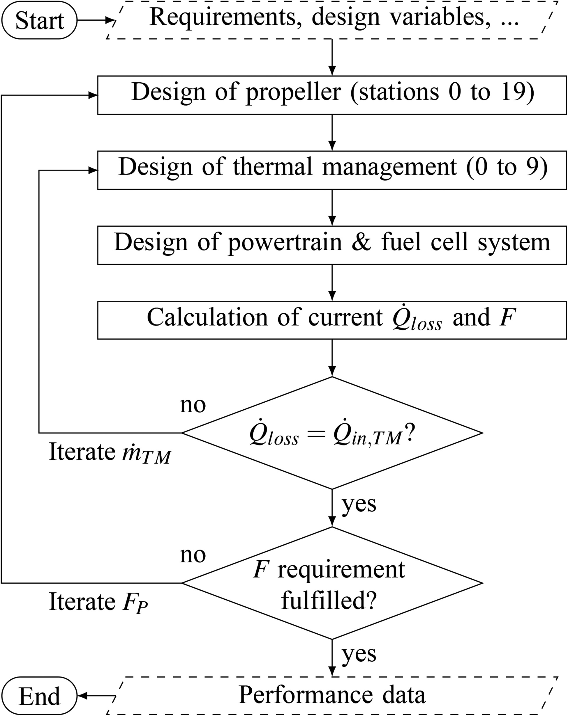
Design calculation process
The flowchart of the design process is shown in Appendix C. It is important to note that some of the variables to be calculated are interdependent. For instance, the power of the cooling air fan
Results and discussion
The design methodology described in this paper is applied to a reference propulsion system. The sensitivities in relation to the thermal management and the overall propulsion system are then discussed by varying three exemplary design variables.
Reference propulsion system
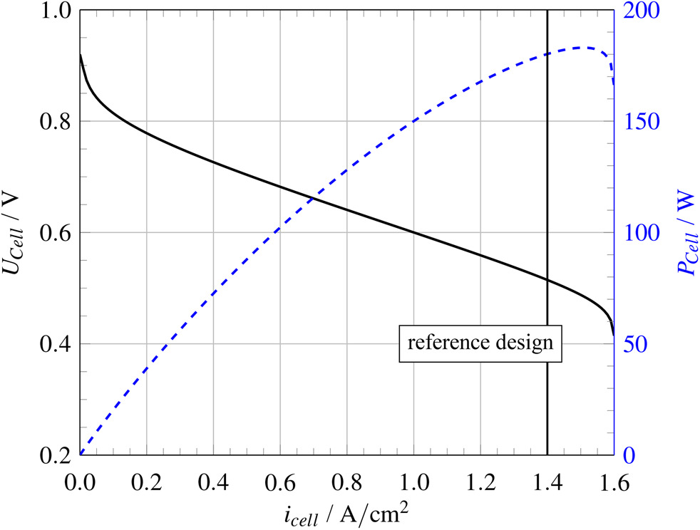
A small four-seater aircraft is used as reference application. Table 1 summarizes the design requirements and environmental conditions for the selected design point during cruise flight. The requirements are derived from typical general aviation aircraft and are otherwise arbitrarily defined. We assume here, that the fuel cell system is designed for the cruise operation point, while a battery provides additional power for take-off and climb. An exemplary design that fulfills the requirements of Table 1 is presented in Table 2. The data utilized for the design of the fuel cell are listed in Appendix D. The resulting polarization curve is presented in Appendix E. The remaining parameters for the powertrain components, which were assumed to be constant for the reference design and the design exploration study, are listed in Appendix F. We now apply the design methodology described and the reference values from Table 2 to the performance requirements and boundary conditions during cruise flight from Table 1. Thereby we obtain the performance data of our reference design as shown in Table 3 that serves as a reference for the following studies.
Table 1.
Performance requirements and boundary conditions during cruise flight.
| Parameter | Value |
|---|---|
| Thrust | 1,000 N |
| Altitude | 3,000 m |
| Ambient condition | ISA + 15 K |
| Airspeed | 85 m∕s |
Design space exploration
By exemplarily varying the design variables
Total pressure ratio of the cooling fan π C
The results of varying
Figure 4.
Plot of m ˙ T M P C F T M , e x t F T M , e x t m T M π C
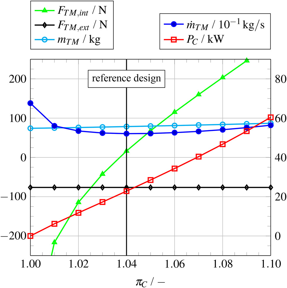
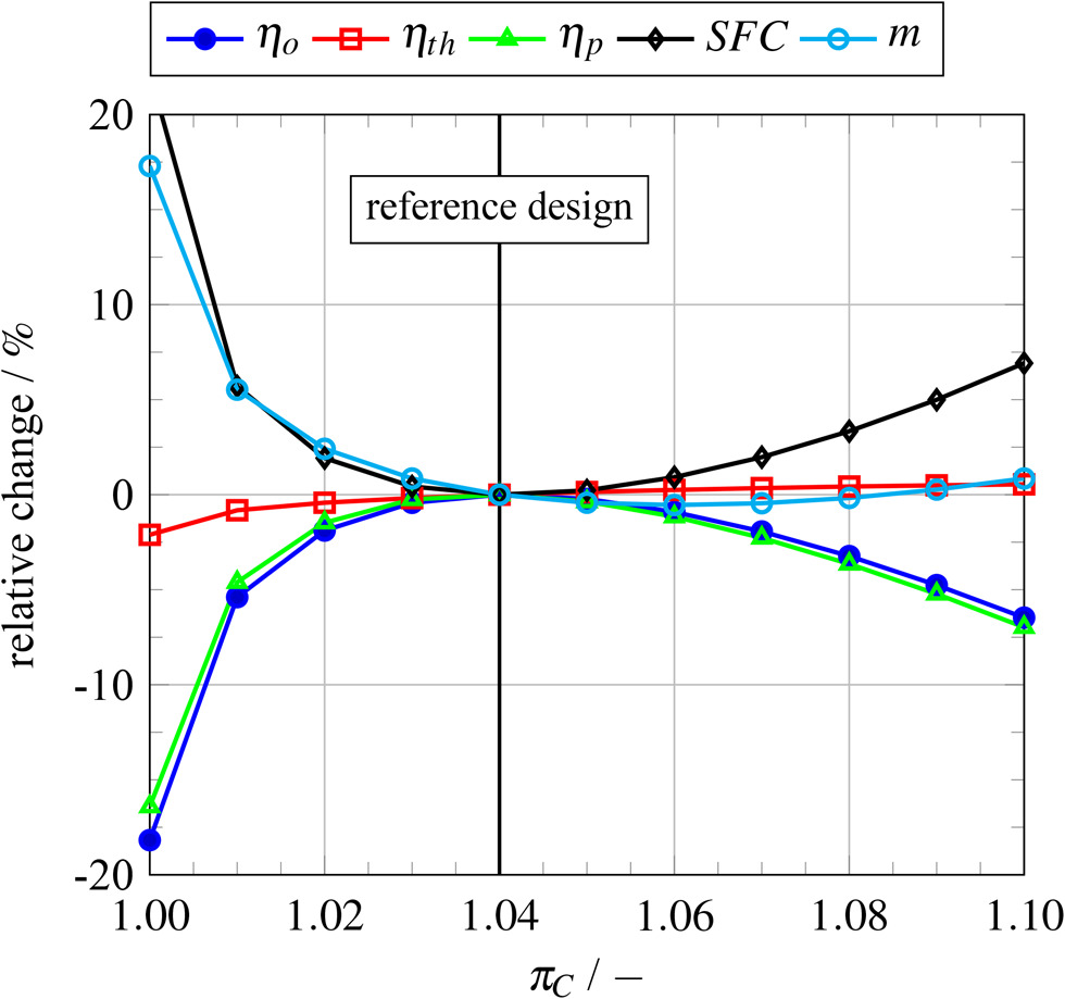
Figure 5.
Plot of the relative change from the reference design (Table 3) of η o η p η t h S F C m π C
Contrary to expectations,
Figure 5 illustrates that
As
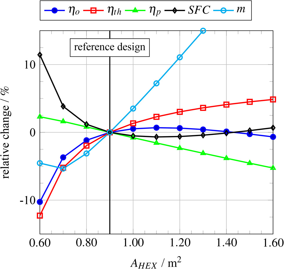
Cross section area of the heat exchanger A H E X
The variation of the heat exchanger area in Figure 6 starts at
Figure 6.
Plot of m ˙ T M P C F T M , e x t F T M , e x t m T M A H E X
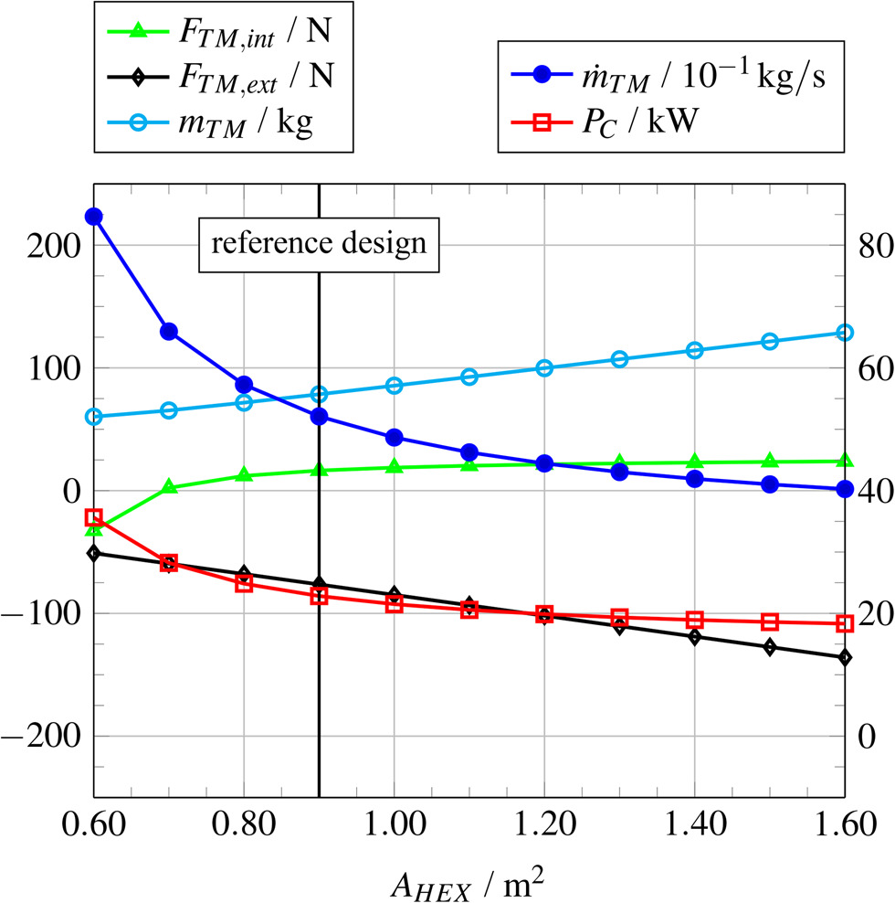
To compensate for the increasing
Figure 7.
Plot of the relative change from the reference design (Table 3) of η o η p η t h S F C m A H E X
Current density of the fuel cell system i c e l l
The cell current density
Figure 8.
Plot of m ˙ T M P C F T M , e x t F T M , e x t m T M i c e l l
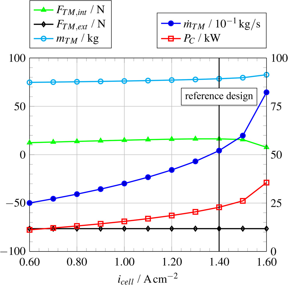
Figure 9.
Plot of the relative change from the reference design (Table 3) of η o η p η t h S F C m i c e l l
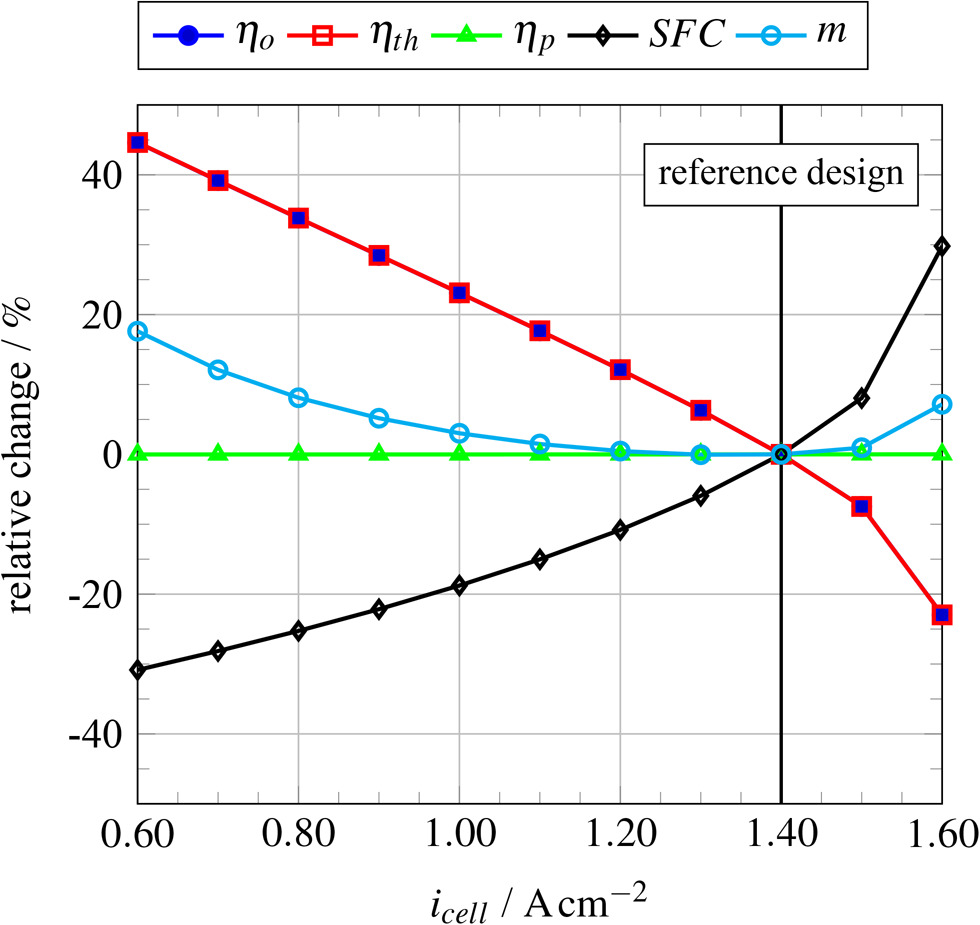
Figure 9 illustrates that
Conclusion
This paper illustrates the integration of the thermal management for a fuel cell propulsion system into the engine performance calculation. The thermal management air path is treated as a separate cycle, similar to conventional engines. Together with the propeller cycle process and the energy conversion from hydrogen to mechanical propeller power, key performance data of the engine performance calculation for the fuel cell powertrain are thus derived. Physically scalable models have been developed for the powertrain and the thermal management components. These models describe the changes in state of the cycle processes and the conversion of energy as a function of their design variables.
The capabilities of the presented method are demonstrated by a design space exploration. First, the fuel cell powertrain system and the thermal management are designed for a small aircraft as a reference application. The reference aircraft engine has an overall efficiency of
The presented method for calculating the performance of fuel cell thermal management systems will be used to analyze key components in more detail in the future. The heat exchanger has a significant impact on the drag, mass, and power demand of the thermal management system. While this study considered a conventional heat exchanger, future enhancements of the method will incorporate new heat exchanger geometries to assess their impact on engine performance. The same applies to the detailed design of the cooling air fan, the air intake, and two-phase cooling concepts. Further potential lies in the coupling of thermal management and hydrogen vaporization. The impact of the thermal management on overall propulsion performance is expected to be even more significant at higher airspeeds. We will therefore extend the method to larger aircraft for up to 50 passengers. The methodology presented thus enables the evaluation of innovative thermal management technologies for fuel cells in aviation.