Introduction

Cavity modes (CMs) are large scale nonsynchronous unsteady pressure fluctuations, which are mainly observed at the cavity exit where the cavity discharge flow interacts with the main flow of the turbine. The nonsynchronous term is used due to the different rotational speed of the CMs when compared to the rotor speed. This nonsynchronous behavior makes it difficult to resolve them with section simulation or current sensor technology. In fact, the CMs have frequencies between the rotor and rotor blade passing frequency (BPF). If these unsteady fluctuations are not controlled, they will be convected into the main flow affecting the performance of the turbine in different ways. The CMs impact has been discussed on different topics such as the profiled endwall performance (Schuepbach et al., 2010), noise (Rebholz et al., 2016), sealing effectiveness (Chilla et al, 2013), rotor loss (Schädler et al., 2016) and also hot gas ingestion into the hub cavity and wheel space (Boudet et al., 2006; Julien et al., 2010).

Although the first openly published study on the rim seal flow was (Bayley and Owen, 1970), but the evidence of the large scale nonsynchronous cavity modes was discussed in detail by (Cao et al., 2004). Recently, (Chew et al., 2018) carried out an excellent review study of the flow mechanisms on the axial turbine rim sealing with a focus on cavity modes.

Schädler et al. (2016) performed extensive experimental and full annular computations studying the migration of the cavity modes into the annulus flow under two purge flow rates. They reported that the reduced rotor loss due to lowering the purge flow rate is weakened by the contribution of the cavity modes. The authors stress the importance of considering the cavity modes during the turbine design process in order to reduce the loss and noise emission by stabilizing the cavity dynamics. The stabilizing effect of the increased purge flow is also mentioned in the study of (Jakoby et al., 2004; Schuepbach et al., 2010). Also, (Chilla et al., 2013) investigated the interaction between the annulus and rim seal flow by simulating a generic high-pressure turbine with different sealing geometry, specifically the overlap-type. They reported that the frequency of the cavity induced vortices is related to rim seal geometry and suggested the stabilization of the modes by either increasing the sealing mass flow or sealing tangential velocity. CMs are also observed by (Boudet et al., 2006) with the frequency of f/f_bld = 0.44. The author relates the generation of these modes to the centrifugal force and pressure gradient inside the hub cavity.

More recently, (Horwood et al., 2018) investigated the flow instabilities at the turbine rim seal using both experimental and computational methods. Their computations showed 16 modes with a rotational speed of 85% of the rotor while the experiments showed 23 < N < 26 modes rotating at 95% of the rotor speed. The authors attribute the origin of these modes to Kelvin-Helmholtz instabilities in the tangential shear layer at the cavity exit. Their finding confirms the reduction in the intensity of the cavity modes by increasing the purge flow rate. But (Gao et al., 2020) relates the cavity modes to the inertial waves attributed with Coriolis forces. By a computational study of three typical rim seal geometries (chute, axial, and radial), they observed large scale fluctuations rotating at an angular speed close to the core flow. Authors believe that due to the complexity and high Reynolds number of the flow, it is difficult to relate the results to the classical phenomena such as Kelvin-Helmholtz instabilities.

In this paper, the impact of different variations on the behavior of the CMs will be studied from experimental investigations. Different cavity geometry modifications such as axial gap change or implementing flow deflectors are taken into account. Furthermore, the pressure ratio of the turbine is altered for three test cases to evaluate the characteristic change in the behavior of the CMs. Eventually, experimental evidences are shown to evaluate the origin of these modes and discuss possible approaches to control their growth.

Methodology

The experiments were conducted on the “LISA” axial turbine test facility at the Laboratory of Energy Conversion (LEC) at ETH Zurich. Figure 1 depicts the layout of the test facility.

Figure 1.

Schematic of the “LISA” test facility.

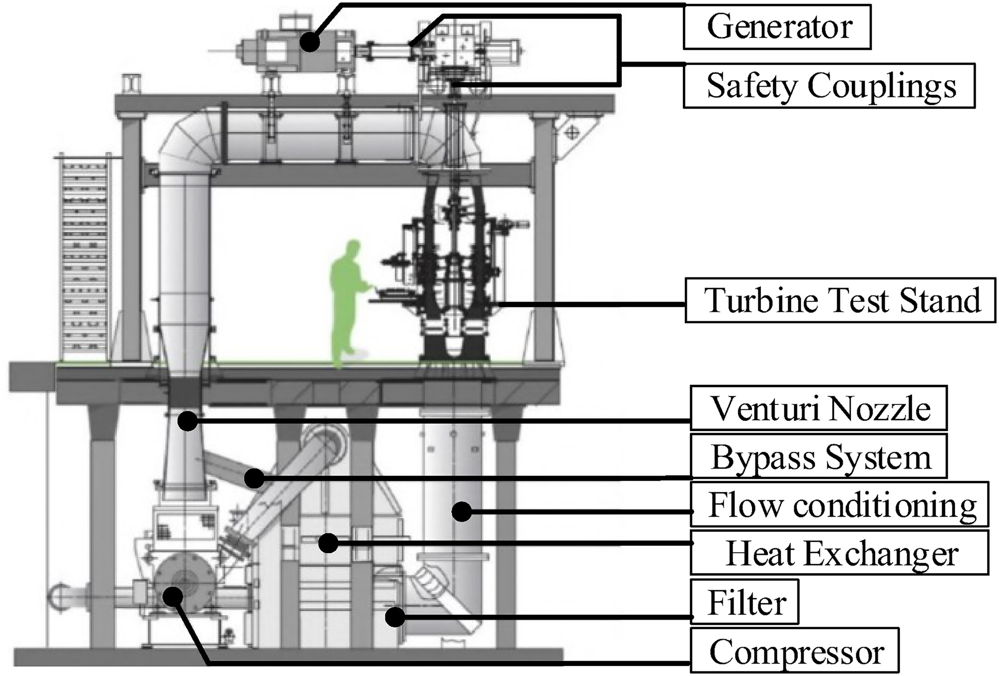
The core airflow was produced using a centrifugal compressor upstream of the test section. Later the flow passes through a heat exchanger, which is used to control the temperature of the flow at the turbine inlet. Electrical power generated from the test turbine was fed back into the electrical grid through the generator, which was placed after the turbine and the gearbox. The generator was also responsible for maintaining the rotational speed of the turbine, which was 45 Hz for all cases. For more details regarding the test facility, please refer to (Sell et al., 2001).

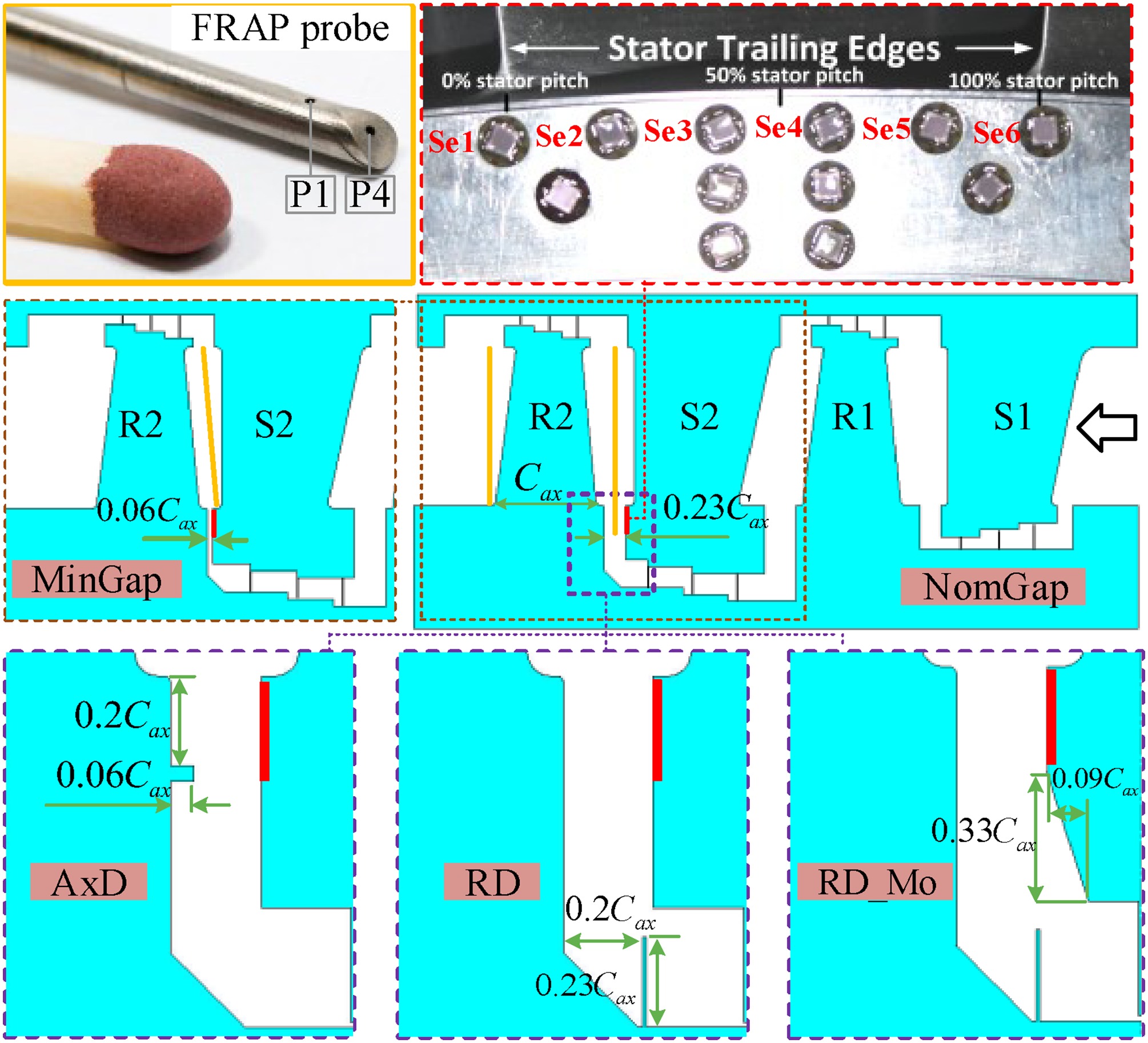
A two-stage turbine configuration representative of a high-pressure steam turbine was designed and tested. The 2nd stage was the test section, while the first stage provided a controlled flow and imposed the multi-stage effect. The hub cavity of the 2nd stage had large dimensions, which is a necessity in the steam turbines to compensate for thermal expansions. Figure 2 depicts the geometry of different test cases. Two test cases with different axial gap distance at the cavity exit, which are referred to as the nominal gap (NomGap), and minimum gap (MinGap) cases with 23% and 6% axial gap normalized to the 2nd rotor axial chord, respectively. Then, three cases were introduced by implementing different flow deflectors on the base geometry of the NomGap case. The axial deflector (AxD) case has a deflector aligned with the flow path with a height of 6% and a depth of 20% inside the cavity. This feature would interact with the rotor pumping flow and the boundary layer of the rotating wall. The radial deflector (RD) case has a radially aligned deflector deep inside the cavity exit. This design aims to keep the cavity flow away from the rotor wall, which is expected to delay the boundary layer generation and the thickness. In order to minimize the high-speed jet created between the radial deflector and stator hub cavity wall, a modified design (RD_Mo) was also introduced by creating a cut on the stator wall to open up the gap and allow for smoother penetration of the cavity flow. The deflectors were designed considering the boundaries given by the industrial partner to assure the applicability of the modifications. All other geometrical details of the test cases were identical.

Figure 2.

Schematic of experimental test cases as well as measurement technologies that are used.

The operating conditions of the turbine are summarized in Table 1. Turbine exit static pressure was measured at the hub wall of the 2nd stage exit using seven circumferentially distributed pressure taps. Also, four total pressure pitot tubes installed at the upstream of the 1st stage stator to measure the inlet total pressure. The ratio of the inlet total pressure to exit static pressure was defined as the turbine pressure ratio and was controlled with a standard deviation of 0.07%. The nominal pressure ratio of the turbine is 1.35. For some test cases, this parameter was altered to 1.3, 1.4. 1.42, 1.45, and 1.47 to study the off-design conditions. The upstream heat exchanger also controlled the total inlet temperature of the turbine. The inlet temperature of 313.15 ± 0.3 K was kept constant for all test cases.

Details of the measurement technologies and the locations they were used are also depicted in Figure 2. The measurements were completed using a Fast Response Aerodynamic Probe (FRAP) and wall-mounted unsteady pressure transducers. FRAP probe had two actual P₁ and P₄ sensors, and two virtual P₂ and P₃ sensors, which were measured by rotating the probe along its axis (Pfau et al., 2002). A trigger installed on the rotor shaft was used to synchronize P_1–4 for any synchronous fluctuations. The sampling frequency of the probe is 200 kHz. Probe measurements were conducted at the 2nd rotor inlet and outlet planes. The outlet plane was always radially aligned. The mid-plane had to be tilted by −3 degrees for the MinGap case to avoid damaging the probe by the rotor. Each measurement plane consisted of 1,705 grid points (55 radial × 31 circumferential points) to cover a full stator pitch. The unsteady pressure transducers were installed at the stationary wall of the 2nd stage hub cavity exit. These sensors were implemented to measure the characteristic parameters of the CMs without blocking the flow path.

Results and discussion

The current study discusses the characteristic behavior of the CMs at different conditions. CMs are considered as pressure waves with the mode number of N which are rotating with a certain speed of ωCM. A single unsteady pressure sensor would capture the frequency spectrum of these modes but will not provide any information regarding the speed or mode numbers. As an example, the measured averaged frequency spectrum from the Se1∼6 at the stationary wall is shown in Figure 3 for the NomGap case. The horizontal axis is frequency normalized with the rotor blade passing frequency (BPF = 2,340 Hz), and the vertical axis is pressure normalized with the pressure of the BPF. At this location (−3% span), the peak amplitude of the CMs is 3.6, which shows the strength and importance of the CMs. In addition to BPF and frequency of the CMs, engine orders 1 and 2 (EO1&2) can also be recognized in the frequency spectrum.

Figure 3.

Frequency spectrum of the CMs from wall-mounted Se1∼6 (averaged) for the NomGap case at the nominal pressure ratio of 1.35.

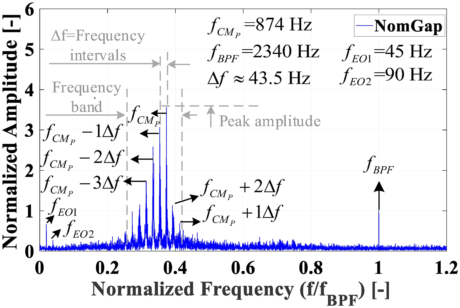
The frequency content of the CMs has an intricate pattern that needs to be analyzed if a physical mechanism is going to be explained. The amplified frequency band due to the CMs is from 0.25 to 0.45 (585 to 1,053 Hz) for this condition. In the frequency band, in addition to the peak frequency (fCMP), eight other distinct peaks can be observed, with their associated frequencies differing by a multiple of a constant number, respectively, which will be referred to as frequency interval (Δf). These parameters will be affected by design or operational variations, which will be assessed in detail.

The rotational speed and the mode number of a single CM with a specific frequency can be measured using a pair of sensors measuring simultaneously. If the measured phase angle of a particular CM is plotted versus the actual geometrical angle difference between the sensors, then the slope of the line would be the mode number. By using more than two sensors (6 sensors (Se1∼6) for this study), the accuracy of the measured mode number will be higher. Figure 4 depicts an example of the measured phase angle for two frequencies of fBPF and fCMP.

Figure 4.

Measured phase angle from Se1 to 6 for the frequencies of peak cavity mode and BPF (NomGap case).

The fBPF is plotted to show the accuracy of using six sensors. For this frequency, the mode number is the blade count (52). If two sensors were used, then the mode number would fluctuate between 48 to 53, but with six sensors, the slope is 52.01, which is accurately the expected mode number. This approach also suggests that using two sensors on a broader gap would give a better estimation of the mode number. For example, if Se1 and Se6 were used to evaluate the mode number, then the results would be 52.6, which is closer to the expected value. Nevertheless, the maximum distance between the sensors is limited by the highest frequency that needs to be resolved. For fCMP the calculated mode number is 20.1 (≈20), which corresponds to a rotational speed of the CM of 43.3 Hz (3.8% slower than the rotor speed). It is interesting to mention that this rotational speed is relatively close to the observed frequency interval of 43.5 Hz.

For the MinGap case, the pattern is considerably different. Figure 5 demonstrates the averaged frequency spectrum from Se1∼6 at a nominal pressure ratio (PR) of 1.35. The fCMP for the MinGap case is shifted down to 0.25 (620 Hz), which is 29.1% smaller than the fCMP for the NomGap. Also, while the rotational speed of the fCMP was reduced from 43.3 to 34.4 Hz (−21%), the peak mode number only decreased from 20 to 18. More interestingly, the frequency intervals are approximately 34.5 Hz, which are again comparable to the rotational speed of the fCMP.

Figure 5.

Averaged frequency spectrum of pressure fluctuations from the Se1∼6 sensors for the MinGap case at the nominal PR of 1.35.

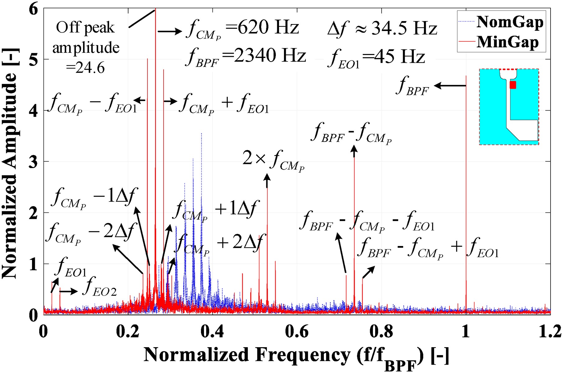
Regarding the peak amplitude, it is 6.8 times higher than the NomGap case while the amplitude of fCMp±nΔf fluctuations drop much faster when compared to the fCMP. The frequency spectrum of the MinGap case shows new contents that were not observed for the NomGap case, which are mainly the interaction frequencies. The distinct structure of the fCMP leads to an interaction with the rotor frequency showing fCMP±fnEO in the spectrum. Also, the fCMpinteracts energetically with the fBPF leading to fBPF±fCMP. The spectrum becomes more complicated when the new frequencies start interacting with each other, as shown in Figure 5. In addition, the 1st harmonic of the fCMp is observed which was not the case for the NomGap.

The impact of the geometrical modifications is depicted in Figure 6. All three deflectors were successful in suppressing the CMs. The AxD case is considered the most effective approach due to the complete suppression of the CMs. The RD and RD_Mo cases reduced the CMs amplitudes down to 0.5 and 0.68, respectively. For these cases, a broader range of frequencies is amplified, showing 18 and 19 peaks for RD and RD_Mo cases, respectively.

Figure 6.

The impact of cavity geometry modification on the behavior of the CMs from wall-mounted Se1∼6.

To mimic the off-design condition, the PR of the turbine has been altered from the nominal PR of 1.35. This test was performed for NomGap (strong CMs), RD (weak CMs), and AxD (No CMs) cases. The variations in the frequency spectrum for the NomGap and RD cases are shown in Figure 7.

Figure 7.

The impact of turbine PR change on the frequency spectrum of the CMs averaged from Se1∼6.

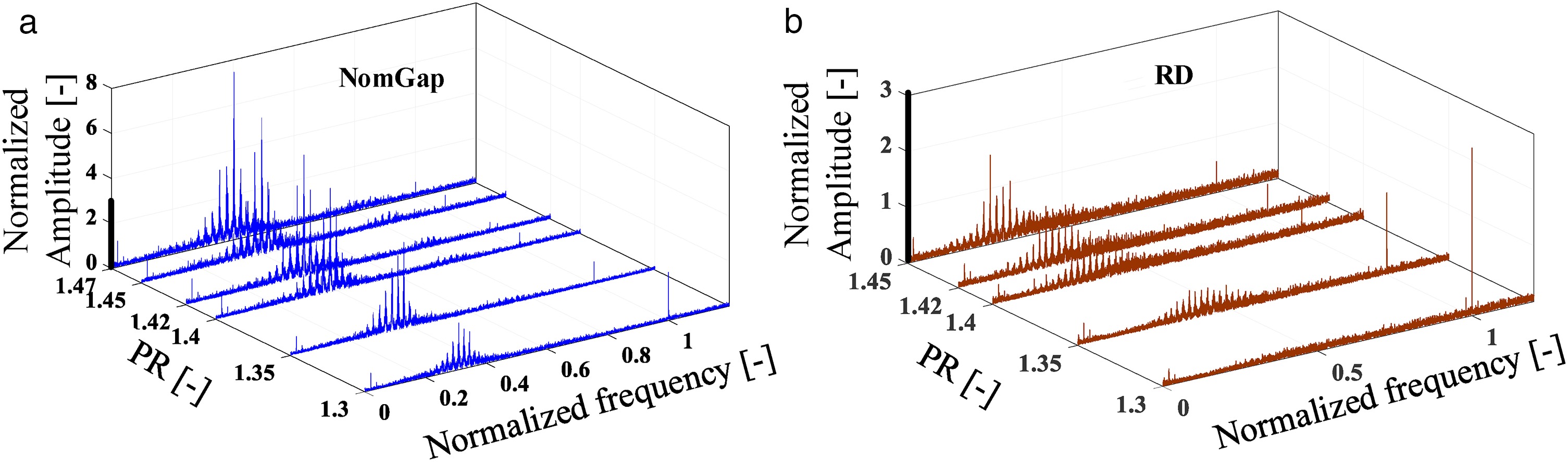
The amplitude of the CMs grows by increasing the turbine PR. For the NomGap case, at the maximum PR of 1.47, the normalized peak amplitude is 7.8, which is 2.2 times higher compared to the nominal PR. Also, the frequency band gets wider due to the increased frequency interval between the peaks. However, the number of peaks stays constant at 9. Also, a gradual frequency shift occurs toward higher frequencies. The RD case shows a similar response but on a smaller scale. Comparably, the RD case shows 3.2 times higher amplitude at PR = 1.45 compared to nominal PR. The amplified frequency band also gets broader, but the frequency shift does not show a clear pattern. Interestingly, for the AxD case, even at elevated PR of 1.47, no sign of the CMs were observed. The AxD case remains effective even at off-design conditions.

In order to quantify the strength of the CMs, both the amplitude and the associated amplified frequency band must be taken into account. For this purpose, the Power Spectral Density (PSD) of the pressure signal from S1∼6 is calculated and the band power for the amplified frequencies due to the CMs is integrated for different conditions. The calculated power is then normalized with the NomGap power of the CMs at the nominal PR of 1.35. Figure 8 depicts the variations in the normalized band power. It’s worth mentioning that for the NomGap case at nominal PR, the band power of the CMs (which is normalized to 1 in Figure 8) is significantly higher than the band power for the BPF.

Figure 8.

The impact of turbine PR change on the band power of the CMs.

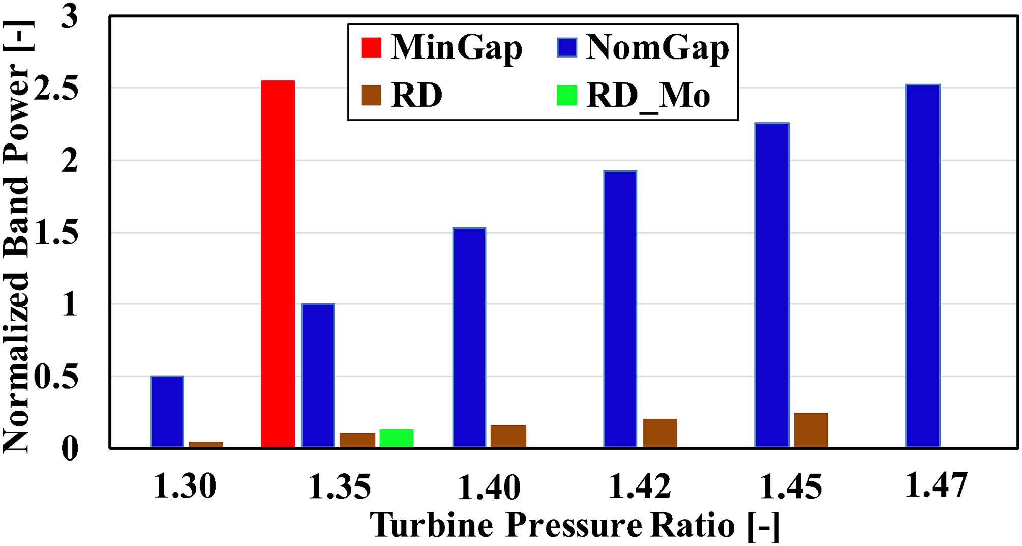
At the nominal PR, the MinGap case shows 2.6 times higher band power compared to the NomGap case. The high amplitude of the peak frequency and intense interactions with rotor and BPF cause the observed increase in band power. Also, as it was expected, a significant drop in the band power is calculated for the RD and RD_Mo. These cases show 0.1 (90% lower) and 0.12 (88% lower) band power compared to the NomGap case, respectively. Also, the AxD case, which is not shown here, has negligible band-power.

Regarding the impact of PR change, the RD and NomGap cases are plotted. For both cases, the band power increases by the increase in PR. Compared to the nominal PR, the NomGap case shows 2.5 times higher value at maximum PR of 1.47. The higher amplitude of the CMs and the broader range of amplified frequencies causes this increase. More importantly, this increase is almost equal to the MinGap case at nominal PR, which shows the importance of off-design condition. Also, reducing the PR to 1.3 leads to 50% reduction in the band power. For the RD case, at the minimum PR of 1.3, the CMs were not observed (see Figure 7b). Also, at the maximum tested PR of 1.45, the band power is 0.24, which is 1.2 times the band power at nominal PR.

Another interesting topic to discuss is the damping ratio. According to half-band power criteria (Zhang and Hoshino, 2019), the non-dimensional damping ratio (ξ) can be estimated using the frequency spectrum of a resonance. To calculate this, first the frequency band in which the half of the power is accumulated is found. Then, the half frequency band is divided by the peak resonance frequency (fCMP) to calculate the damping ratio. Table 2 summarizes these results.

The MinGap case has the smallest damping equal to 0.0008. The low damping for the MinGap case is reasonable, considering the observed distinct peak. For the NomGap case, damping is 0.028, which is 35 times higher. A pressure wave that is generated at the cavity exit would travel towards the rotating and stationary walls of the rotor and stator and hit the walls and bounce back. Moving through a fluid would lead to the damping of the wave energy. For the NomGap case, the gap is four times wider, and therefore, the pressure wave must travel a longer distance to reach the wall causing substantial damping.

Regarding the deflectors, damping is increased by 3.4 times relative to the NomGap case, which shows a minor impact of the deflectors compared to the axial gap change. PR change also has a negligible impact on the damping. The slight decrease is due to the positive shift in the peak resonance frequency. In the RD case, the peak frequency shifts slightly to lower values, and for this reason, the damping increase with increasing the PR.

The relation between the characteristic parameters of the CMs and the base flow conditions at the cavity exit is evaluated in this section. In the past, the tangential velocity at the cavity exit (Chilla et al., 2013) and also the mass flow ratio of the cavity flow (Jakoby et al., 2004; Schuepbach et al., 2010; Schädler et al., 2016) was found to be affecting the CMs behavior. The goal here is to analyze these two factors in the turbine and try to relate the variations to the CMs. The NomGap case is selected for this analysis. For both parameters, the measurements in the nominal PR is used for approximation in off-design condition. The maximum tangential velocity at 2% span is measured to be 116 m/s. Considering the mass flow of the turbine, which is directly measured at each PR, and also the flow angle at nominal PR, the tangential velocity is estimated at increased PRs. For the mass flow of the cavity, the following equation is used from (Axel Pfau, 2003):

In this formula, the static pressure and temperature at the cavity inlet and outlet are measured with the probes. Regarding the seal geometry, this formula only considers the seal gap size (A). The discharge coefficient (C_D) needs to be multiplied with the ideal mass flow to calculate the actual value. For this, only the computational studies can be used. From computations, the cavity mass flow ratio is 0.85% at nominal PR, which leads to a discharge coefficient of 0.36. These geometric parameters remain constant at different PRs, and the pressure and temperature can be estimated from the measured turbine operating conditions. Figure 9 demonstrates the variations in the relevant turbine parameters as well as the characteristics of the CMs.

Figure 9.

The impact of turbine PR on (a) variations in turbine parameters, and (b) The characteristic parameters of the peak frequency of the CMs.

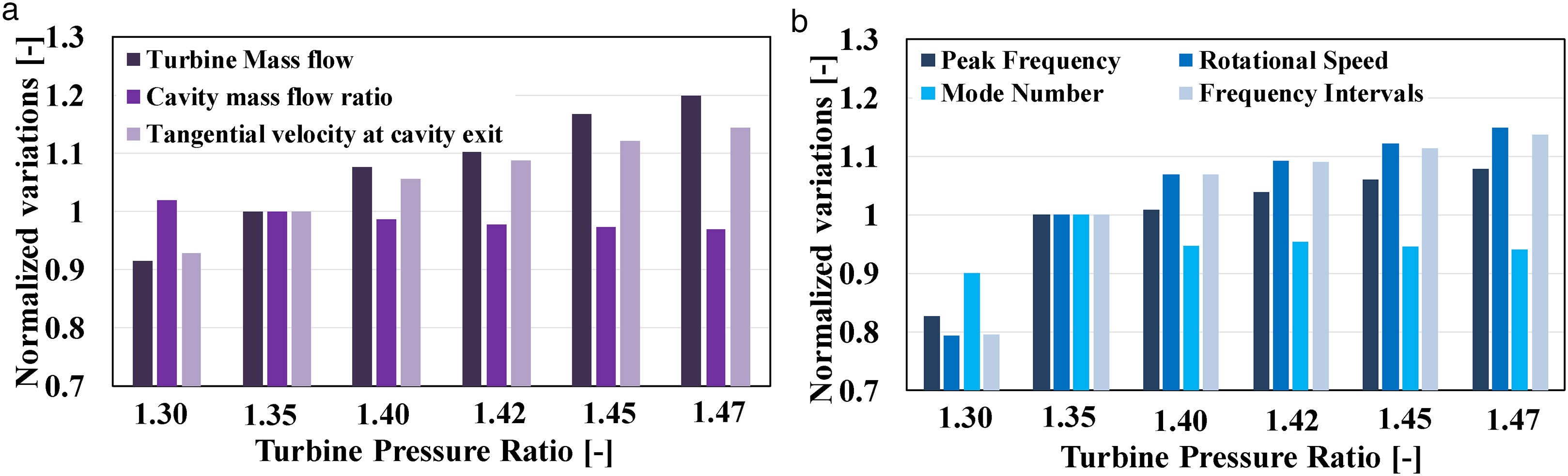
An 8.8% increase in the turbine PR leads to a 20% increase in the mass flow of the turbine. Although the cavity mass flow increases as well, but the dominant increase in the turbine mass flow drops the mass flow ratio by 4%. The change in the mass flow ratio can be considered minimal. The peak tangential velocity, on the other hand, increases by 14% from 116 m/s to 132 m/s. Interestingly, the rotational speed of the CMs also increases by almost the same amount. In fact, the variations in the rotational speed of the CMs is linked to the tangential velocity variations. In addition, the peak mode number, which was 20 for nominal PR, drops to 19 at PR = 1.40 and then remain constant. At the minimum PR, the mode number is 18, which is also a minor change. Therefore, the frequency shift is mainly driven by the increase in the rotational speed of the CMs, which is driven by the tangential velocity of the base flow. Another interesting fact to mention here is that the above PR = 1.42, the CMs speed actually exceeds the speed of the rotor itself (9.6% faster than rotor at maximum PR). This has not been reported before. Finally, the variations in the frequency intervals show a similar pattern to the rotational speed. In fact, as it was observed at nominal PR, for the elevated PRs, also the frequency intervals are comparable to the rotational speed.

So far, the characteristic parameters of the CMs were only discussed for the peak frequency. It would be encouraging to calculate the mode numbers for other peaks in the frequency spectrum and study their relation to the frequency intervals. Figure 10 demonstrates the mode number of the multiple peaks at different operating conditions and geometrical variations. For each peak, a frequency range of ±4 Hz was evaluated based on the half-band power method. The mode number is then calculated at the frequency range of the peak. The markers show the averaged mode number for each peak, and the error bars are the standard deviation from the averaged value. For each case, a set of mode numbers are amplified, which their difference is approximately 1 (ΔN≈1). For the MinGap case, five mode numbers from 16 to 20 are amplified in which the N = 18 has the highest amplification. For the NomGap case at nominal PR, the mode numbers are from 14 to 22 with a peak at 20, and at maximum PR same mode numbers are amplified, but the peak amplitude is at N = 19.

Figure 10.

The mode number of multiple peaks of the CMs and their dependency on the geometrical and operational variations.

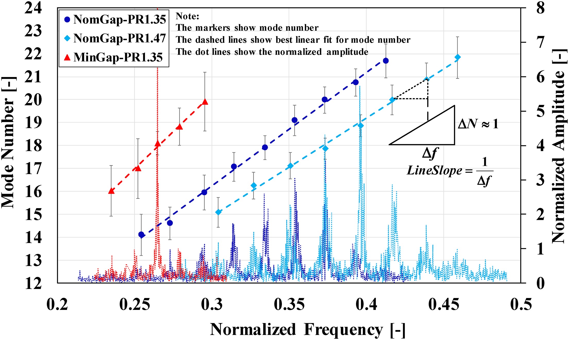
But interesting to consider is the linear change in the mode number versus the frequency. A small triangle is shown to discuss the importance of this linear relation and the slope of the line. Since the difference between the mode numbers is approximately 1, then the slope of the line would be inverse of Δf. Also, observations show that the Δf is basically equal to the rotational speed of the CMs. From MinGap to NomGap at maximum PR, the slope decreases gradually. This means that the rotational speed increase, which is consistent with the measured values. This finding also has a practical importance since the CMs speed and mode number can be estimated using only one sensor. In the frequency spectrum of a single sensor, the rotational speed would be the frequency intervals between the peaks. Therefore, the mode number will also be calculated by dividing each peak frequency through the rotational speed (which was shown to be constant for all mode numbers). This approach is applicable only if the intervals are not equal to rotor frequency because then it will be due to interaction between the peak CM and the engine order fluctuations.

From all different conditions which were studied, at the nominal PR, the MinGap case is the most affected geometry. In this part, the relation between the CMs and stator and rotor hub flow structures such as wake and passage vortices will be evaluated from the FRAP probe data. Similar to wall-mounted sensors, the P₁ and P₄ sensors of the FRAP probe can also be evaluated to study the fluctuations. In Figure 11a, the normalized amplitude of fCMP is shown at the stator exit from the P₁ sensor of the FRAP. The normalization factor is similar to the previous plots. The P₁ sensor is always aligned to the flow direction, and therefore, it’s variations are representative of the total pressure fluctuations. Also, the time-averaged total pressure coefficient (Cpt=PtPtturbineinlet) is shown to identify the location of the loss structures.

Figure 11.

(a) The normalized pressure fluctuations for the peak cavity mode from P₁ sensor and, (b) the time-averaged Cpt, both at S2 exit and from FRAP probe for the MinGap case.

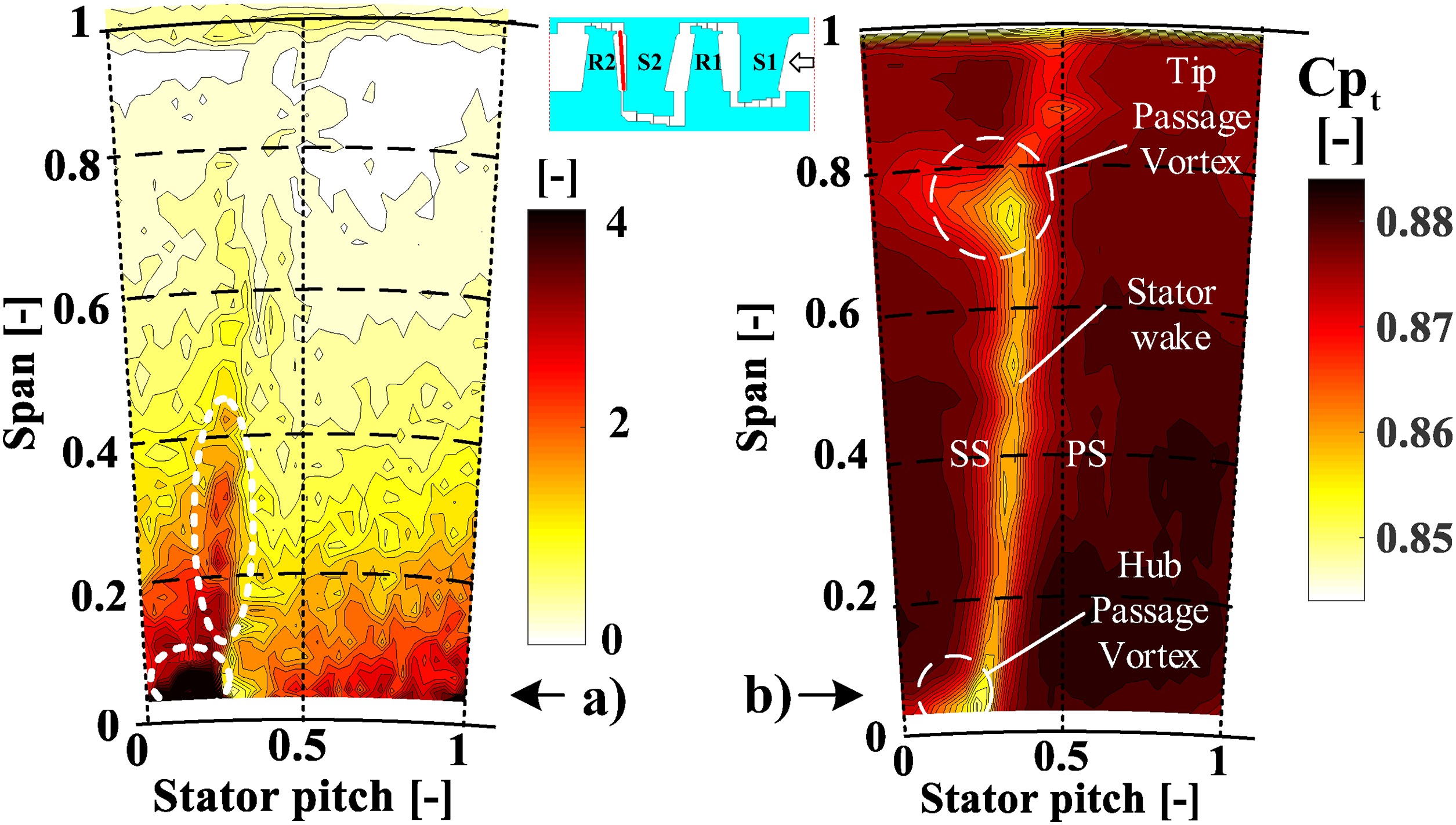
Three main flow structures are the hub and tip passage vortices and also the stator wake. It is clear that the amplitude of the fCMP is higher at the hub passage vortex and also at the wake. The suction side of the stator wake is more affected than the pressure side. The interesting fact to consider is that near the hub, the probe tip is actually located at the upstream of the cavity exit (−3° tilting of the probe) but still shows high fluctuations amplitude for the CMs, which is comparable to the fluctuations at the stator wall measured by the wall sensors. This means that despite the high Mach number near the hub, the CMs can travel upstream of the cavity exit and influence the condition at the stator passage. In addition, due to the strength of the CMs, they are observed up to 100% of the span at the stator exit plane.

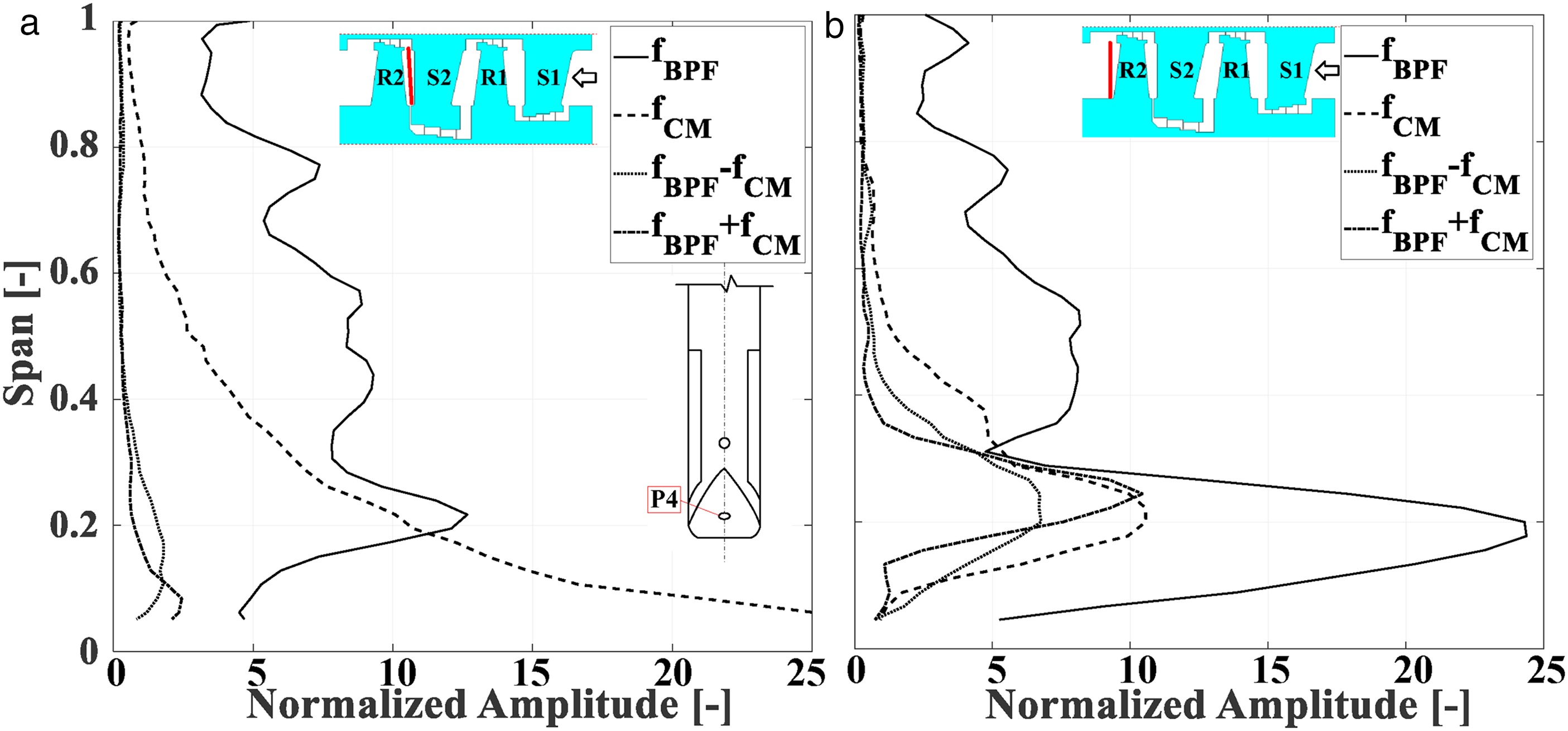
The interaction frequencies, which were discussed from wall-mounted sensors in Figure 5, can also be studied from the FRAP probe sensors in the passage. These interactions, which are due to rotor passing, are more intense in the P₄ sensor of the FRAP probe. Figure 12 depicts the normalized amplitude of the fluctuations for different frequencies. The fBPFis also shown to compare the amplitudes with the blade passing fluctuations. At the rotor inlet (Figure 12a), below 18% span, the fluctuations are completely dominated by the fCMP. At minimum span location, the amplitude of the peak CM is five times stronger than the BPF. However, the interaction frequencies of fBPF±fCMP are relatively small. Moving to the rotor exit (Figure 12b), the amplitude of the interaction frequencies grow considerably to be as strong as the fCMP. Also, at 30% span the CMs and their interactions have comparable strength as the BPF. The peak amplitude of the CMs is observed at around 25% span while the BPF peak is at a slightly lower span location (20% span). Eventually, the CMs presence is observed up to about 60% span.

Figure 12.

The normalized amplitude of pressure fluctuations from the P₄ sensor of the FRAP probe at (a) rotor inlet and, (b) rotor exit.

In Figure 12, the variations are shown in a stationary frame of reference. In order to see the interaction of the CMs with hub flow structures of the rotor, the fluctuations must be studied in the rotor frame of reference. For this purpose, the measured total pressure signal is split into three parts as below:

Pt¯ is the averaged total pressure, Pt~(t)and′Pt(t) are the phase-lock averaged pressure (synchronous with rotor blade passing) and random part of the fluctuation referred to RMS, respectively. The RMS of the total pressure fluctuations at the rotor exit is shown in Figure 13 for the NomGap and MinGap cases.

Figure 13.

The time-averaged (2D plots) and time&mass averaged (1D lines) of the total pressure RMS at the rotor exit from FRAP probe.

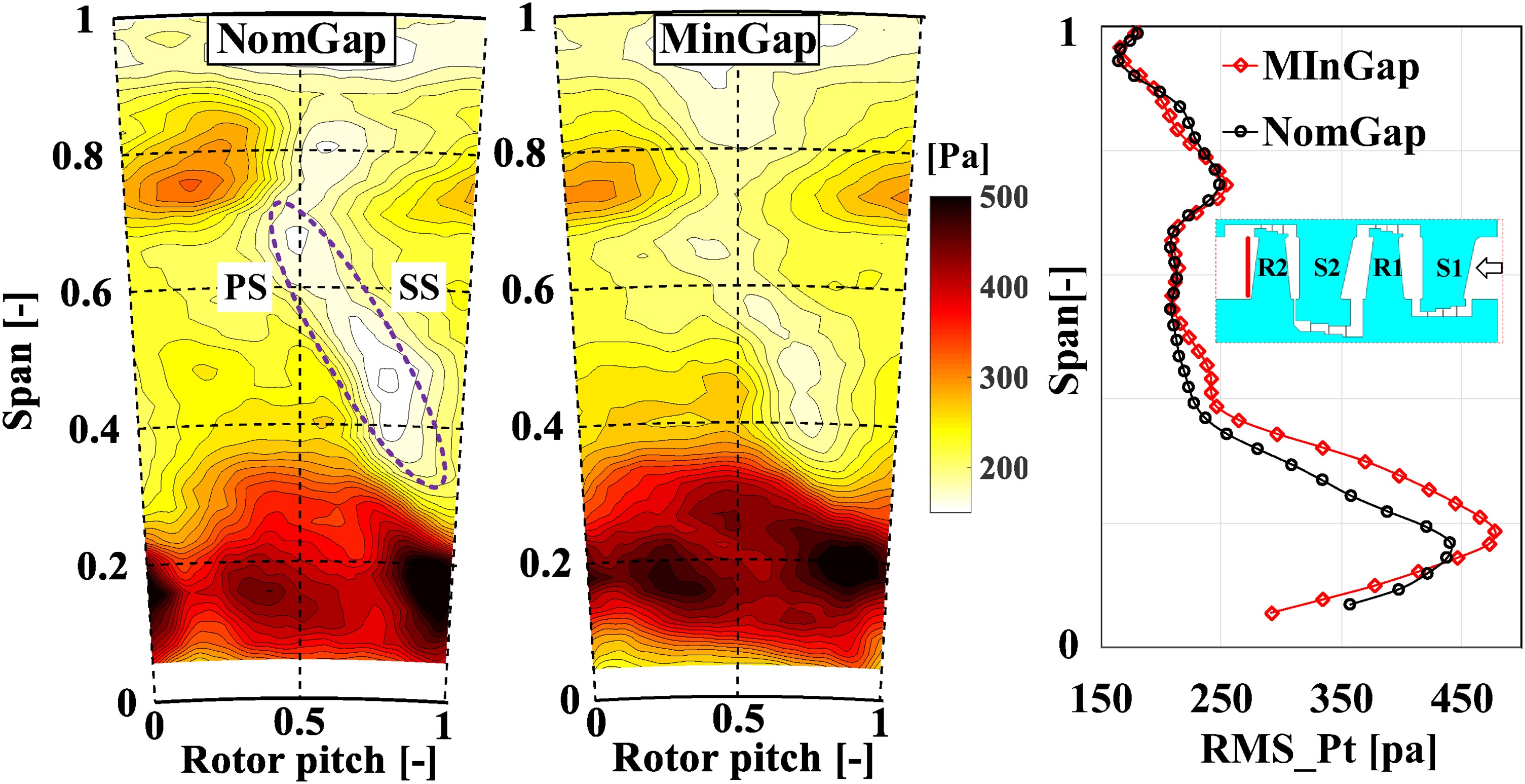
Both time-averaged and mass-averaged comparisons are plotted. In the time-averaged plots, it can be seen that the Pt_RMS is higher below 40% span and from 70 to 90% span. The first is due to hub flow structures, and the later is related to tip flow structures. Also, there are two local peaks at the hub region between 10% to 30% span. The first one, which has a core at around 35% rotor pitch, is related to hub trailing shed vortex. The second one with a peak at around 80% rotor pitch is because of the hub passage vortex.

In the mass-averaged plot, a local peak is present at 19% span for the MinGap case, which is shifted down to 16% for the NomGap case. This can be linked to the higher radial velocity at the hub cavity exit for MinGap case (narrow gap creates a stronger radial jet), The RMS differences between the MinGap and NomGap cases are apparent below 55% span. This is also an indication from the impact of the CMs, considering the fact that they were also observed slightly below the 60% span in the frequency spectrum. In the mass-averaged plot, up to 14% span, the NomGap case has slightly higher RMS, but from 14% to 53% span, the MinGap case shows a higher RMS value with a peak of 478 pa. At the same span location, the RMS value for the NomGap case is 420 pa (13.8% lower compared to MinGap case). In the time-averaged plots, it is clear that this increase mainly occurs at the local peaks in the circumferential direction, which are due to hub flow structures. The total averaged value of the Pt_RMS along the span is 276 pa for the MinGap case and 260 pa for the NomGap case, which means a 6.2% lower value.

So far, it was shown in Figures 8 and 9 that the increase in the turbine pressure ratio would lead to a higher shear layer velocity difference and also stronger CMs. Such effect is expected if the instabilities are of Kelvin-Helmholtz type. According to Rayleigh theorem (Rayleigh, 1879), the existence of an inflection point in the velocity profile of parallel flow is a necessary (but not sufficient) condition for instability. The Rayleigh criteria were later extended by (Fjørtoft, 1950). The theorem states that; in order to have the instability, the necessary (but still not sufficient) condition is that the inflection point corresponds to vorticity maximum. To investigate this criterion, the mass-averaged tangential velocity (Vθ), the velocity gradient (∂Vθ/∂r), and the normalized amplitude of the CMs at the cavity exit region are depicted in Figure 14 for the NomGap case from the FRAP probe.

Figure 14.

The relation between the tangential velocity and the CMs amplitudes at the 2nd hub cavity exit for NomGap case measured by the FRAP probe.

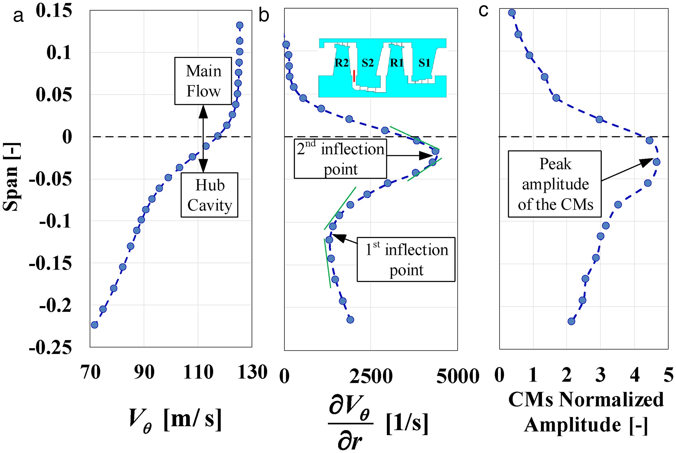
The tangential velocity gradient is basically representing the axial vorticity. Two inflection points are present in the shear layer at −11% span and −3% span. Based on the Rayleigh theorem, both of these points are a candidate for instability, but considering the Fjϕrtoft theorem, only the inflection point at −3% span is an unstable condition since it also corresponds to a vorticity maximum. Interestingly, the radial distribution of the CMs amplitude, which is also plotted from the P₄ sensor of the FRAP probe, shows a maximum at −3% span. The velocity profile of the current shear layer can be modelled with a hyperbolic tangent function. The stability analysis of this velocity profile is studied by (Michalke, 1964) and discussed in different textbooks, such as (Charru, 2011). In Figure 15, the dispersion curve for the unstable modes is depicted.

Figure 15.

The dispersion curve of the unstable modes for a hyperbolic tangent shear layer velocity profile (Michalke, 1964).

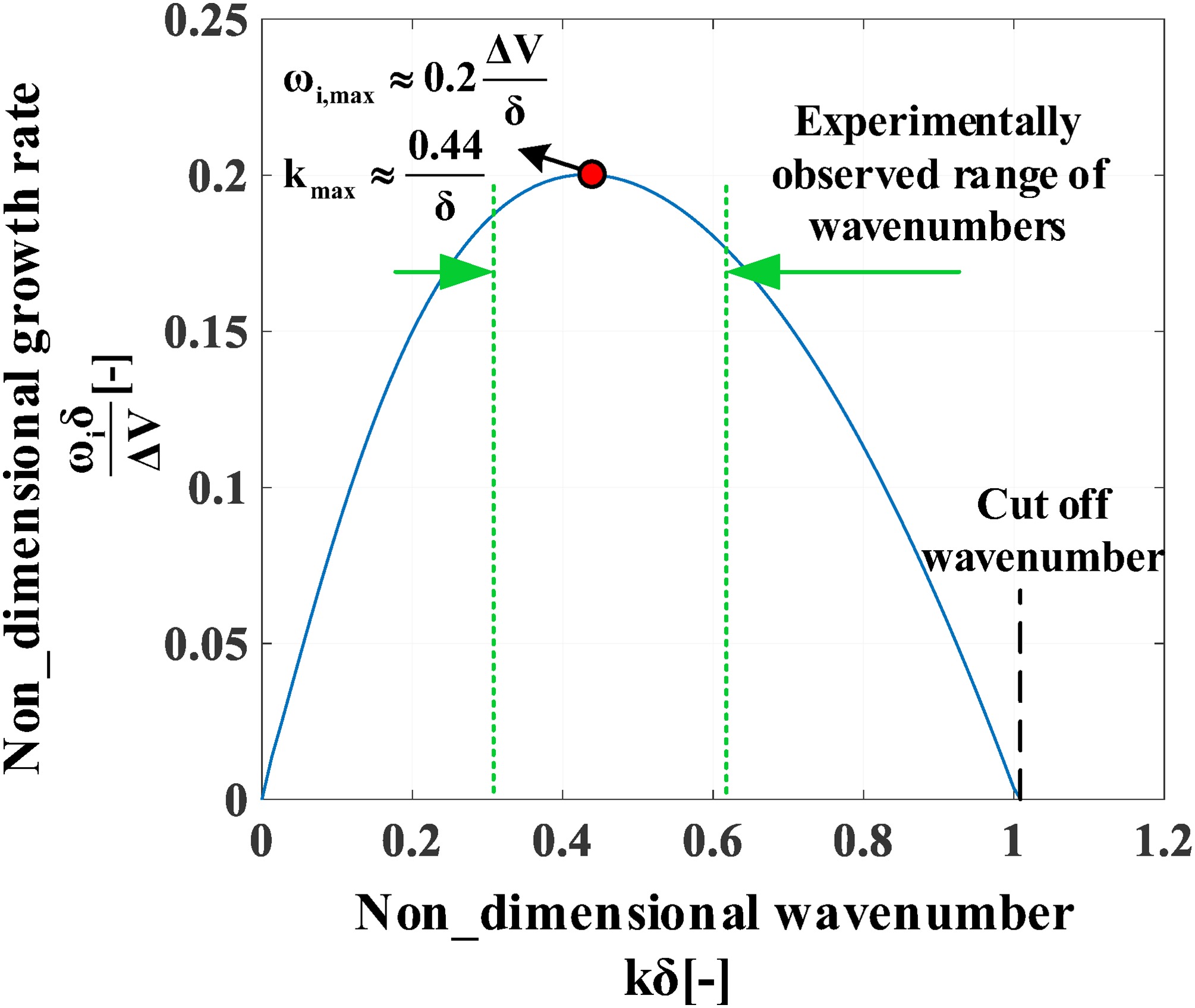
According to (Michalke, 1964), the non-dimensional wave number with the highest growth rate is kδ=0.44. The mode number can be converted to wavenumber by dividing it with hub radius (k = N/r). Considering the thickness of the shear layer for the NomGap case (δ=7.5mm) , this corresponds to a mode number of N≈18, which is fairly close to the peak mode numbers observed from the experiments. More importantly, the maximum growth rate of instabilities (ωi,max) is linearly proportional to the velocity difference in the shear layer, meaning that an increase in the velocity difference would lead to higher growth rates. In the cavity interaction zone, several factors can change the shear layer velocity difference. The tangential velocity of the main flow can be altered by the turbine pressure ratio, as shown before. Also, using design criteria such as forced-vortex below 10% span of the stator exit can significantly reduce the tangential velocity difference in the interaction zone. On the other hand, the minimum tangential velocity inside the cavity mainly depends on the rotational speed of the rotor. Hence, an increase or decrease in the rotational speed can also provoke or lessen the velocity difference, respectively. In addition, increasing the mass flow of the cavity by actions such as purge flow (air turbine) or clearance opening (steam turbine) can drop the cavity tangential velocity, enhancing the growth of instabilities. Such an effect can also be seen in the work of (Schädler, 2019) when the increase in the purge flow from 0 to 0.8% led to stronger CMs while the tangential velocity difference became stronger due to the drop in the cavity rotational velocity.

Conclusions

This paper presented the sensitivity of the turbine hub cavity modes (CMs) on the geometrical variations and also at the off-design condition. The experimental tests were conducted at a two-stage axial turbine with the hub cavity design of a high-pressure steam turbine. The axial gap at the hub cavity exit has been varied, and also different deflectors were implemented. Also, the turbine pressure ratio (PR) has been varied to study the off-design conditions.

For the MinGap case with an axial gap of 0.06 C_ax, the CMs showed a distinct peak in the frequency spectrum, and intense interaction with the stator and rotor hub flow structures were observed. Four times increase in the axial gap for the NomGap case led to considerable damping of the CMs. The peak amplitude was 6.8 times smaller, but a broader range of frequencies was amplified. The band-power was 2.5 times lower, and the damping ratio 35 times bigger. Also, the interaction frequencies were mainly eliminated. But, an 8.8% increase in the PR led to the same increase in the band-power for the NomGap case. Implementing the deflectors was found to be a successful method to eliminate the CMs. A radial deflector deep inside the cavity reduced the band-power by 90% compared to the NomGap case and an axial deflector attached to the rotor wall at the cavity exit, has eliminated the CMs completely.

Although the mode number of the peak frequency was constant at 19 ± 1, the rotational speed of the CMs depended on different conditions causing the frequency shift. The speed was closely linked to the tangential velocity of the base flow at the interaction zone. For a 14% increase in the base flow tangential velocity, an equal increase in the speed of the CMs was observed. Interestingly, at increased PRs, the CMs rotational speed exceeded the rotor speed. In addition to the peak mode number, several other mode numbers were also amplified. A linear relation was found between the mode number and the frequency, in which the slope of the line was related to the rotational speed of the CMs.

The variations observed in the behavior of the CMs were mainly concurrent with the variations in the shear layer at the interaction zone. The radial location of the maximum peak of the CMs at cavity exit coincided with the inflection point in the tangential velocity profile. This condition is necessary bud not sufficient requirement to have instability in the shear layer, based on the Fjϕrtoft theorem for Kelvin-Helmholtz instability. Also, the K-H instability suggests that the growth rate of instabilities is linearly proportional to the velocity difference in the shear layer, and decreasing the velocity difference can potentially weaken the CMs.

Nomenclature

Abbreviations