
Introduction
Corner separation is one kind of the 3D separated flows that is commonly observed at the junction of the endwall and blade suction surface within axial compressors. At off-design flow conditions, this separation can appear to be large and localized, which can contribute significantly to the passage blockage. This places a limit on the loading and static pressure rise achievable by the compressor (Gbadebo et al., 2005). Furthermore, once flow separates, the mixing within the separation region, and the mixing of the separated flow with the main passage flow may lead to a considerable stagnation pressure loss and thus reduction in the compressor efficiency (Dong et al., 1986). Therefore, it is necessary for Computational Fluid Dynamics (CFD) to predict corner separation and its consequences with good confidence, in order for it to be used as a reliable design and analysis tool.
Despite the significant advances in the scale-resolving simulation techniques in industrial CFD, RANS is still widely used in the industrial flow simulations, and will remain in high demand at least until the mid-21st century (Spalart, 2015). This is largely because of its cost-effectiveness, numerical robustness, and relatively easy of use. However, several eddy-viscosity based turbulence closure models that are commonly used in industry, such as the Spalart-Allmaras (SA) model (Spalart and Allmaras, 1992) and the Menter's hybrid
To reduce the modelling uncertainties for corner flows, a number of studies have been available focusing on mathematically formulating the nonlinear stress-strain relation for more turbulence anisotropic effects to be realistically modelled, e.g., Pope (1975), Hanjalić and Launder (1976), Gatski and Speziale (1993), Spalart (2000), and Hellsten and Wallin (2009). As explained by Gatski and Speziale (1993), the secondary flow of the second kind, as observed around corners, acts as one of the main physical mechanisms to determine the location of the corner separation onset. In other words, it is observed that the secondary flow driven by the anisotropy in the Reynolds normal stresses extracts momentum from the main passage flow into the corner. This leads to the corner flow being more resistant to the adverse pressure gradient, and thus delays the separation onset. The secondary flow of the second kind can only be captured via the incorporation of higher-order terms in the stress-strain relation. All turbulence closures that are based on the linear stress-strain relation are intrinsically incapable to predict this flow phenomenon.
In the current paper, the primary goal is to investigate the predictive capabilities of a recently developed nonlinear stress-strain relation (Menter et al., 2018) for the secondary flows in corners. This is an explicit constitutive relation which is capable of reproducing turbulence anisotropy without a large penalty on model simplicity, computational cost, and numerical robustness. Coupled with the Menter's hybrid
Model formulation
The explicit quadratic constitutive relation
By adding various forms of the scalar product of second-order tensors (i.e., mean strain-rate tensor and mean vorticity tensor), the Menter et al.'s nonlinear stress-strain constitutive relation is regarded as an explicit extension of the Boussinesq constitutive relation, which is shown as follows (Menter et al., 2018):
where
The Menter's hybrid k − ω / k − ε
The Menter's hybrid
where the production of TKE
The turbulent eddy viscosity is computed as:
Computational details
Flow solver
In the current research, all validation cases are conducted using the ANSYS FLUENT solver, in which the above explicit quadratic constitutive relation is activated and modified via the user-defined macros. The numerical scheme adopted is the pressure-based pressure-velocity segregated algorithm, with the second-order upwind scheme used for the discretization of convection terms in all transport equations. For pressure interpolation the second-order scheme is adopted, and the gradients are approximated with the use of the node-based Green-Gauss method.
The LMFA-NACA65 cascade
A linear compressor cascade which was experimentally investigated by Ma et al. (2011) and Zambonini et al. (2016) at Laboratoire de Mécanique des Fluides et d’Acoustique (LMFA) is used here for the numerical investigation of corner separation. The LMFA-NACA65 compressor cascade consists of 13 NACA65-009 blades mounted at the end of an open circuit subsonic wind tunnel. In the experiment, two strips of sandpaper with 3.0 mm width by 0.3 mm thickness were stuck at an arc length of 6 mm from the leading edge of both the blade suction and pressure surfaces. The aim is to trigger the laminar-to-turbulent transition process at the early stage of the blade surface boundary layer development, whereby removing the impact of boundary layer transition on the downstream corner separation. This contributes to reducing the difficulties of RANS simulations, as no transitional model is needed in addition to the fully turbulent RANS models. The main geometrical parameters are presented in Table 1 (Zambonini et al., 2016).
Mesh
The computational domain for the LMFA-NACA65 cascade is shown in Figure 1. The inlet plane is located at

As the pitchwise periodicity of the time-mean flow was ensured throughout the measurement process (Ma et al., 2011), one single blade passage is simulated, with the pitchwise boundaries set as translational periodicity. Furthermore, as the surface oil flow measurements indicate the flow symmetry with respect to the mid-span (Ma et al., 2011), one half of the blade span is simulated, with the mid-span boundary set as symmetry.
As for the mesh topology, an O4H topology is used, and hexahedral meshes are generated using NUMECA Autogridv5. 376 points are wrapped around the blade and in the near-wall region above the blade surface (O block), 41 points are distributed in the wall-normal direction, with the average
Boundary conditions
As for the mean-flow boundary conditions, the inlet mean velocity profile, flow angle, density, static temperature, and the outlet mean static pressure are prescribed to match the experimental measurements. At inlet, the velocity profile is specified based on a precursor RANS simulation on a zero-pressure-gradient flat plate turbulent boundary layer, with the results of which matching the single hotwire measurements of the cascade inlet endwall boundary layer. Figure 2 compares the computed inflow velocity profile with the experimental measurements (Zambonini et al., 2016). It can be shown that the extracted velocity profile almost reproduces the measurements. The inlet freestream flow parameters are listed in Table 2 and the inlet boundary layer integral parameters are listed in Table 3.
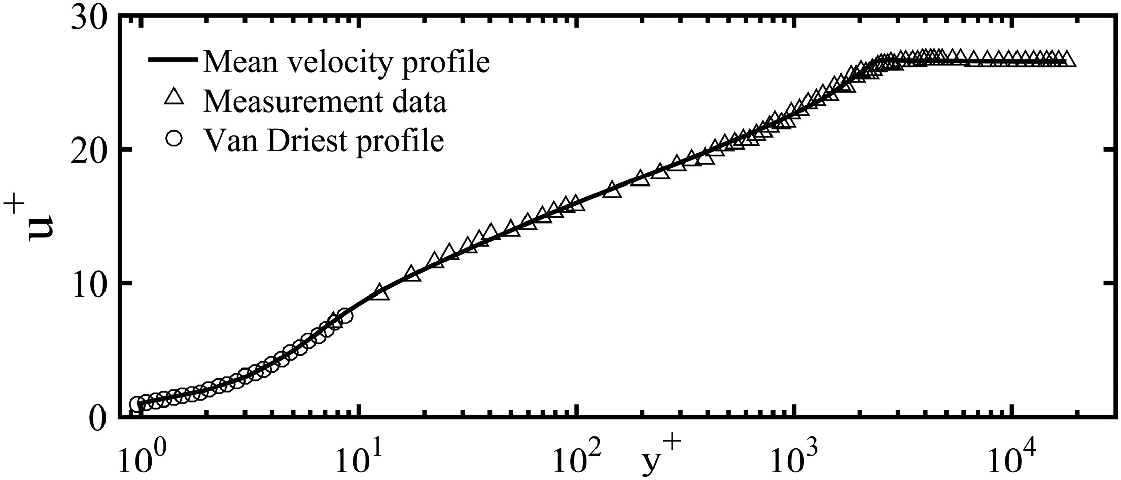
Table 2.
Inlet freestream flow parameters.
| Parameter | Value |
|---|---|
| Chord-based Reynolds number, | 3.82 × 10⁵ |
| Inlet freestream Mach number, M | 0.12 |
| Inlet freestream turbulence intensity, | 0.8% |
Table 3.
Inlet endwall boundary layer integral parameters.
As for the inlet turbulence specification, no detailed hotwire measurements of the fluctuating velocities inside the endwall boundary layer are available. Some uncertainties thus inevitably exist on the treatment of the inlet turbulence boundary conditions. Here the extracted boundary layer velocity profile, as well as the corresponding profiles of turbulent variables (TKE k and specific dissipation rate
Results and discussion
Model validation
In this section, two flow cases for the LMFA-NACA65 compressor cascade are computed and discussed. The purpose is to demonstrate that compared with the BSL-2003 model with the Boussinesq constitutive relation (BSL-2003-L), BSL-2003 with the above-mentioned nonlinear stress-strain constitutive relation (BSL-2003-NL) yields improved predictions of the size of corner separation at various flow conditions.
Case 1 ( i = 0 ∘ )
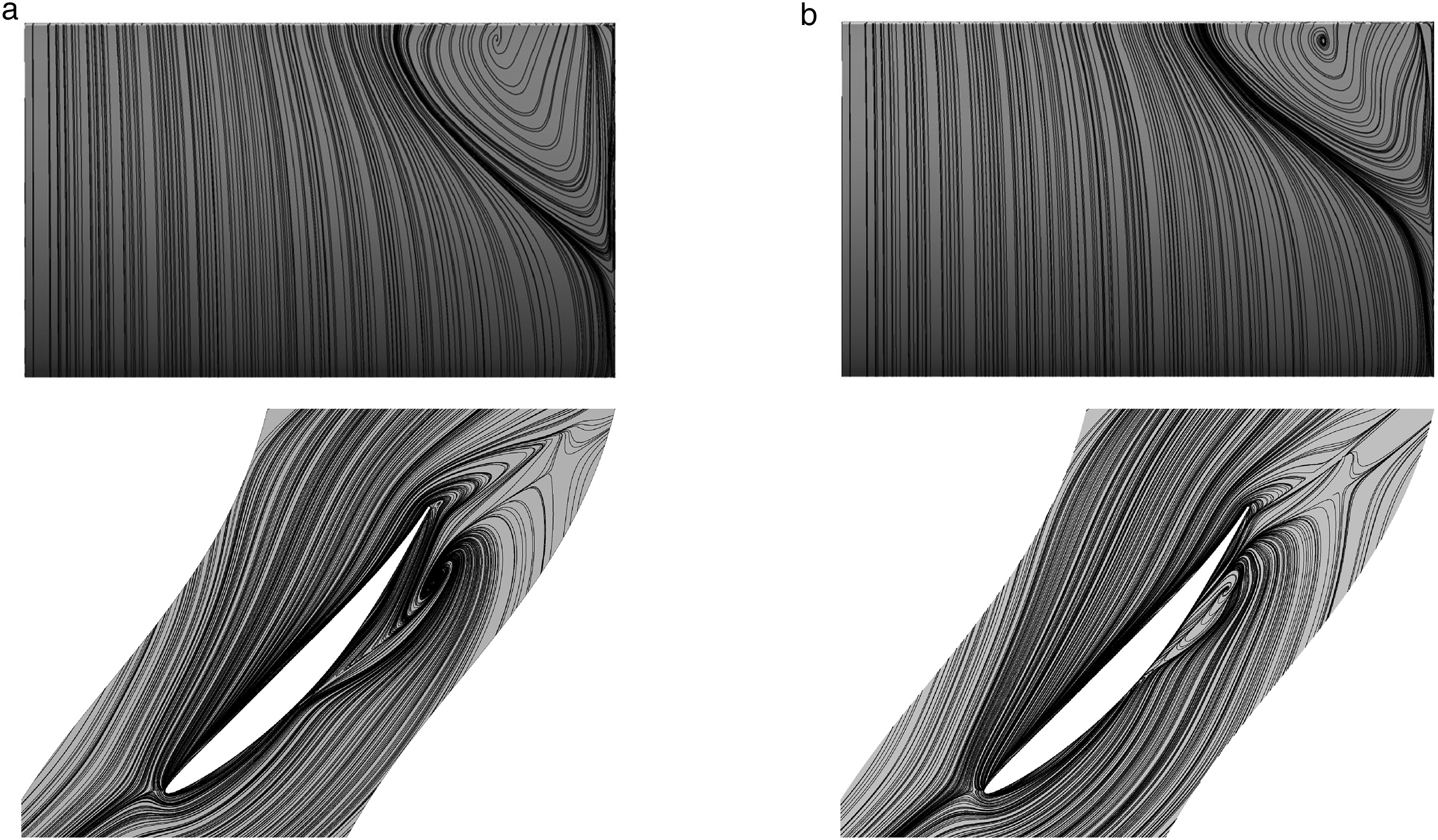
Figure 3 compares the surface limiting streamlines distribution by the BSL-2003-L and BSL-2003-NL models at the design flow condition. As shown on the endwall surface, the boundary layer predicted by the BSL-2003-NL model exhibits stronger resistance to the adverse pressure gradient when migrating to the blade suction surface, thus leading to the smaller size of corner separation and the delayed onset of separation. On the suction surface, the corner separation size predicted by BSL-2003-NL is also shown to be smaller in the chordwise direction than that by the BSL model with the linear Reynolds stress closure. The validation results confirm that the addition of the anisotropic effect of turbulence in the corner region acts to suppress the over-prediction of corner separation.
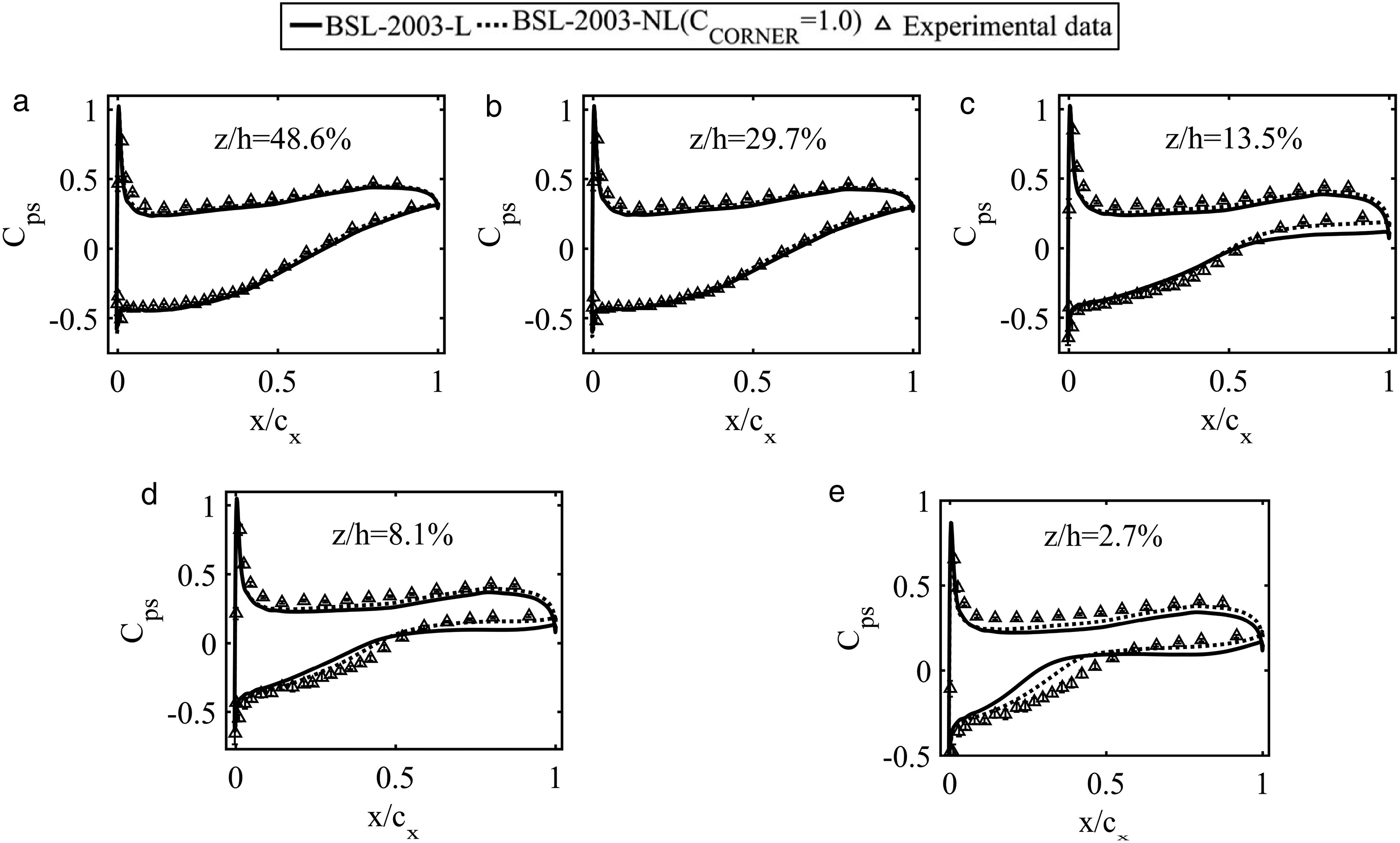
To see how the overpredicted blockage affects the blade loading, Figure 4 presents the distributions of static pressure coefficient Cps on the blade surface. Above the endwall separation region (above

In the endwall separation region, the original BSL-2003 model predicts premature corner separation, while the BSL-2003 model with the explicit nonlinear turbulence closure almost reflects the real flow field. As seen in Figure 4c and 4d, the BSL-2003-L model results in the early boundary layer separation on the suction surface. In contrast, a better pressure recovery is achieved by BSL-2003-NL in the rear part of the suction surface, which matches closely with the experimental measurements. However, in the region closest to the endwall (2.7%h), the BSL-2003-L model results in the overprediction of both the streamwise and pitchwise extent of corner separation, while the BSL-2003-NL model gives results that almost reproduce measurements. This indicates that the corner separation size can be predicted with high accuracy if the anisotropic properties of the flow in the corner region are reasonably modelled.
Overall, it is encouraging to see that the prediction results for corner separation are quite promising. This means that some of the corner separation physics is reasonably captured by addition of the quadratic strain-vorticity term to the Boussinesq constitutive relation.
Next, the validation results of a more challenging flow case are shown to highlight the generality of this nonlinear stress-strain relation for the corner separation prediction.
Case 2 ( i = 2 ∘ )
At the off-design flow condition, as with the design condition, the shrink of the size of corner separation is observed in both the chordwise and pitchwise directions (see in Figure 5). However, the spanwise extent of corner separation turns to be larger than that predicted by the original BSL model. This is due to the increased spanwise velocity close to the blade suction surface within the separation region, a resulting effect of the reconstruction of Reynolds stresses in the spanwise momentum transport equation.
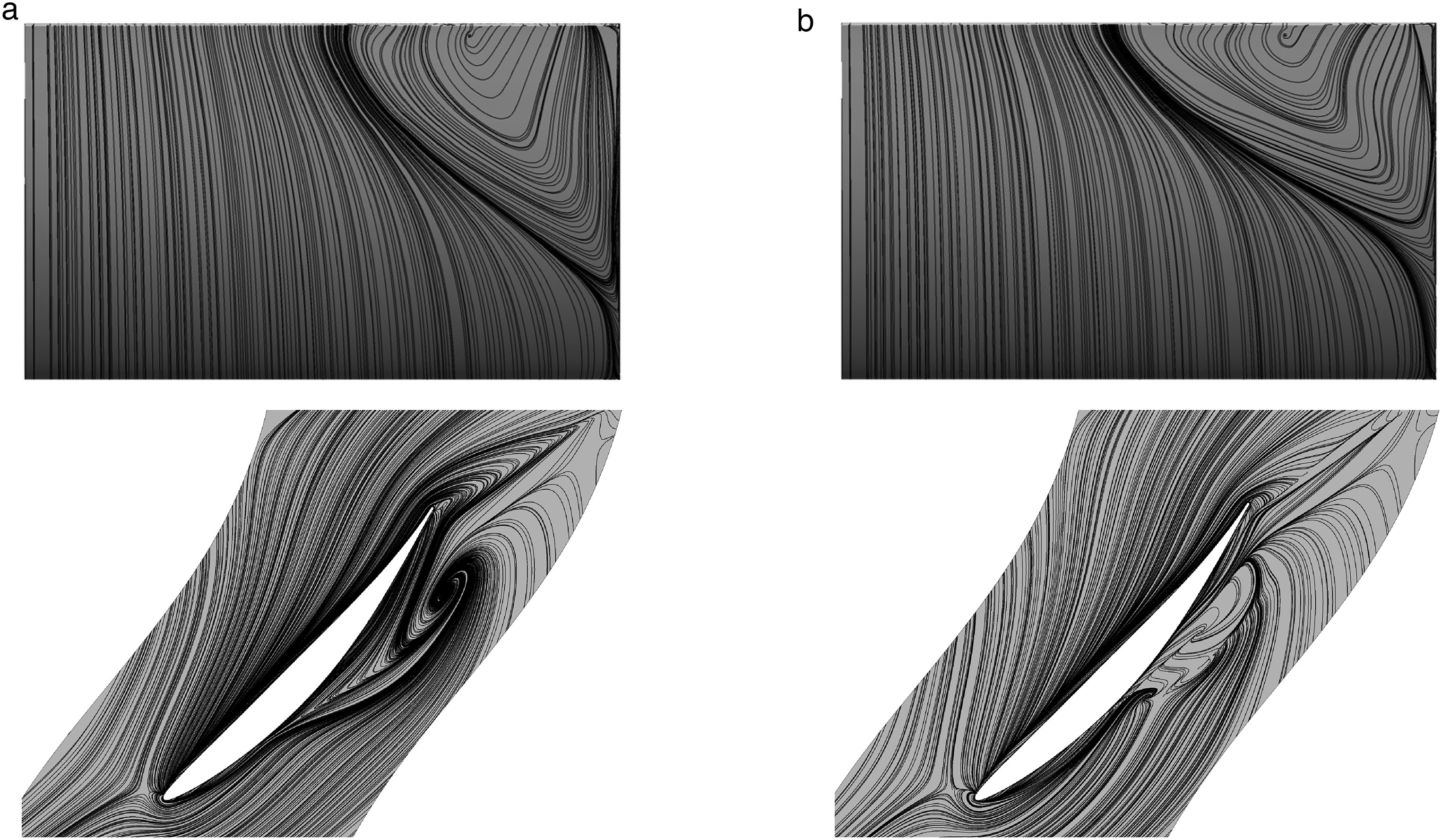
Figure 6 shows the effect of the predicted corner separation on the blade loading distribution. Above the endwall separation (above
However, in the region closest to the endwall (see in Figure 6e), the BSL-2003-NL model predicts the corner separation onset earlier than measurements. One of the physical reasons is hypothesized to be the underestimation of the anisotropic effects of turbulence in the corner separation. As explained in the section “model formulation”,
In the next section, the flow field around the corner region will be analysed to reveal the effect of the anisotropic modification on the mean flow field.
Flow field analysis
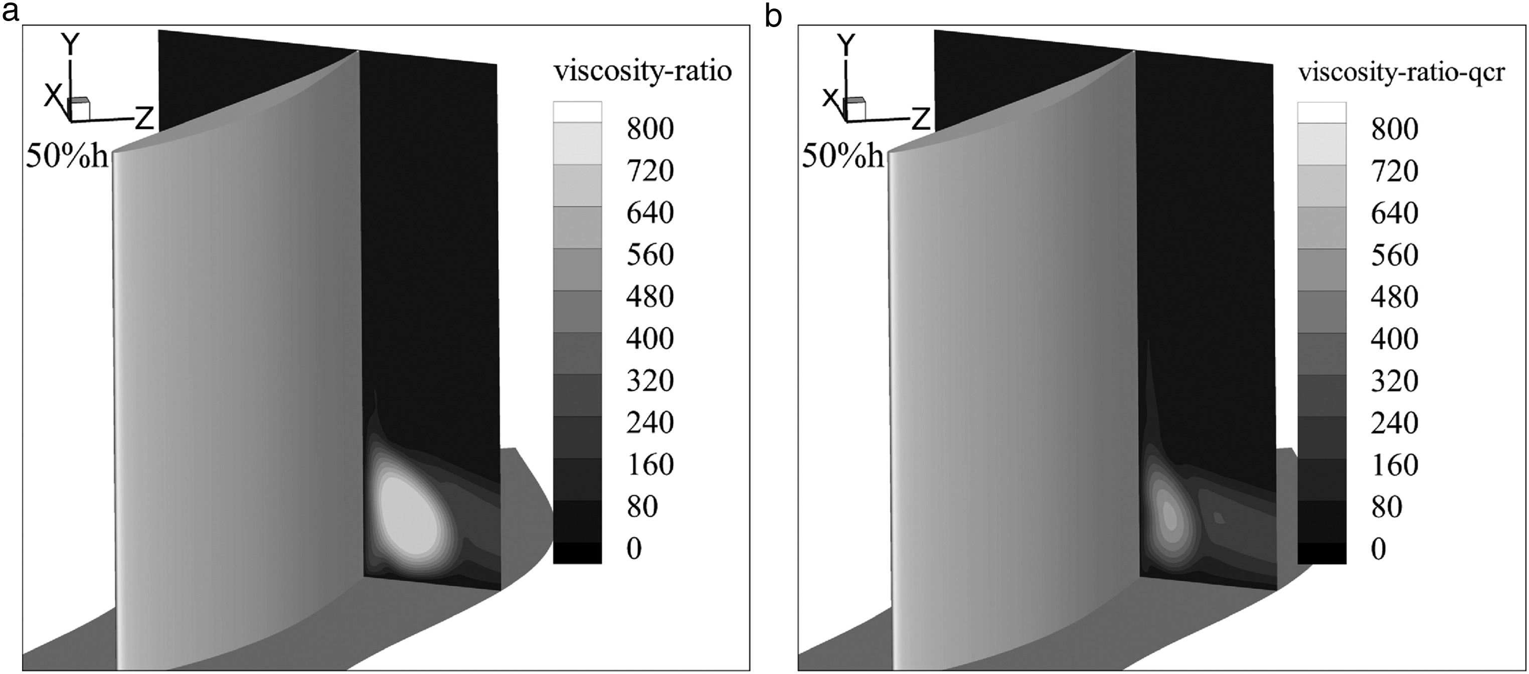
Figure 7 compares the size of corner separation via the distribution of the eddy-to-molecular viscosity ratio
Figure 7.
Comparison of the eddy-to-molecular viscosity ratio ( i = 0 ∘ )
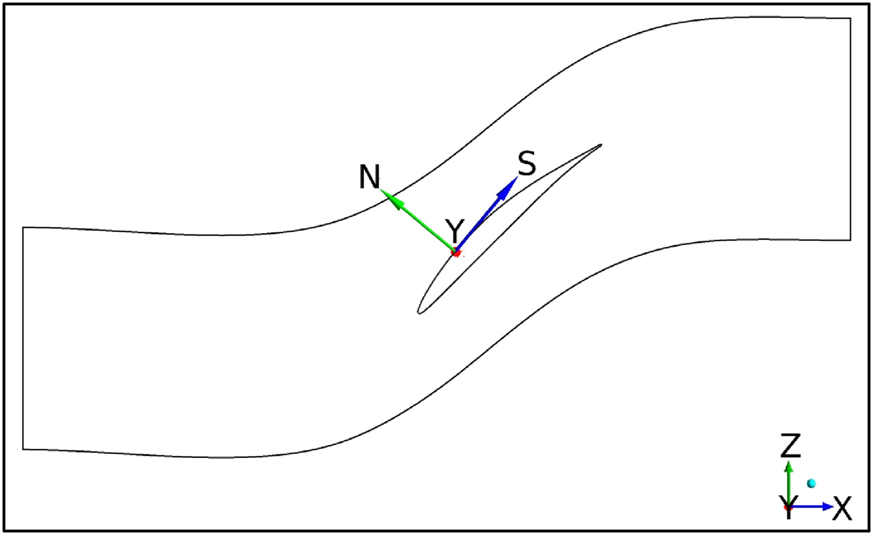
In order to more intuitively compare the mean vorticity field and Reynolds stress field below, a local coordinate system is setup with its three axes s, y, and n respectively representing the streamwise, blade-spanwise, and blade-surface-normal directions (see in Figure 8). The velocity vector, vorticity vector and the Reynolds stress tensor that are computed in the Cartesian coordinate system are projected onto the new local coordinate system.
The generation of vortices in the corner can be described with the use of the streamwise (s axis) vorticity transport equation. With the assumption of incompressible and steady, this equation can be written as (Perkins, 1970):
(8)
where
According to Perkins,
In the discussions below, the effect of the explicit anisotropic modification on the mean vorticity field is first illustrated by checking the streamwise vorticity source terms
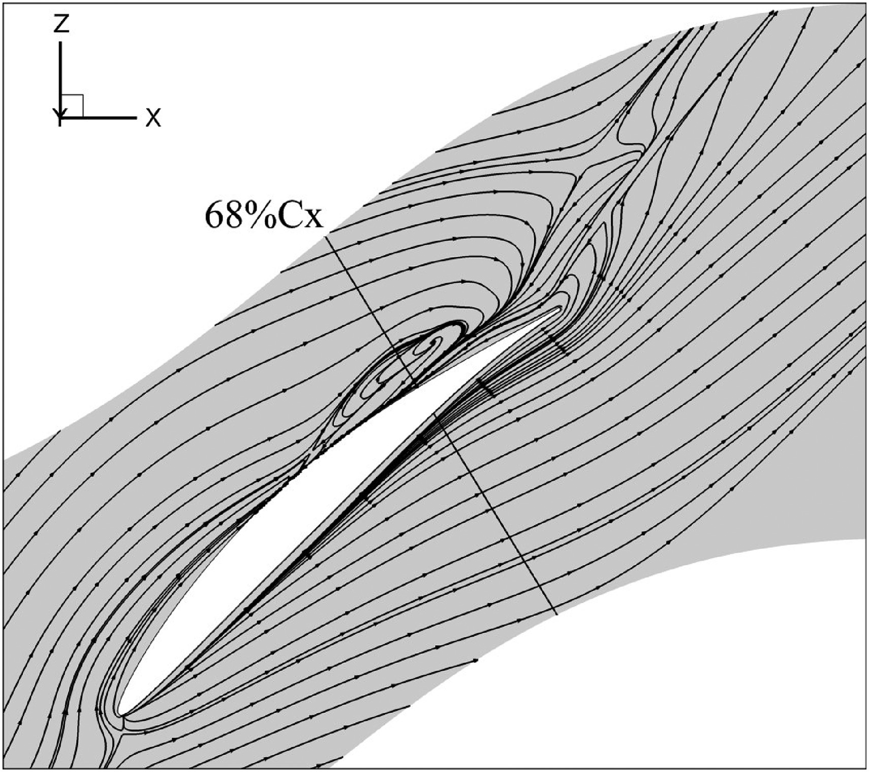
Figure 9 shows one selected cut plane that is normal to the blade camber line, i.e.,
Figure 9.
Endwall surface friction lines, BSL-2003-NL, i = 0 ∘

Figure 10 shows the distribution of

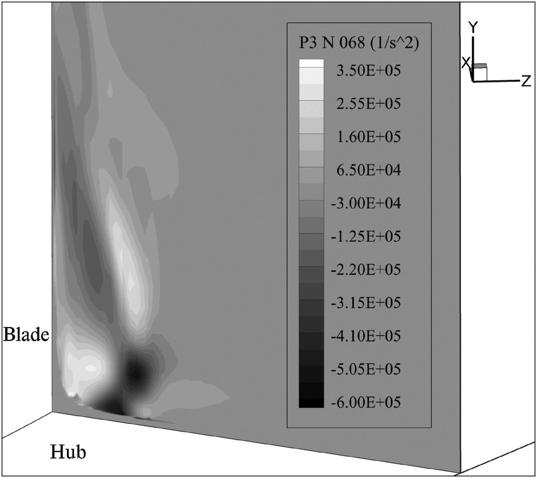
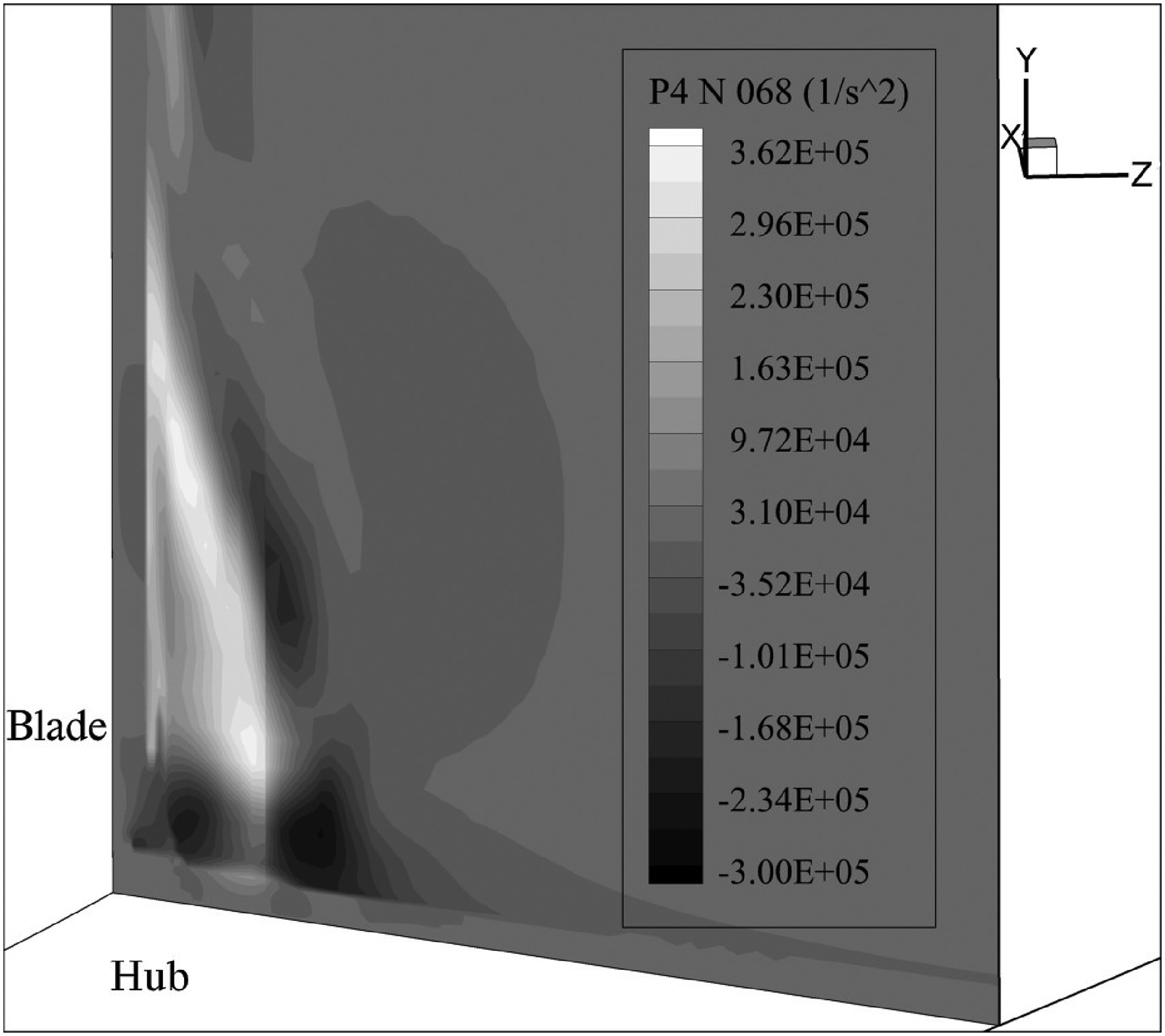
Figures 11, 12, and 13 show the distributions of the non-linear part of the source terms
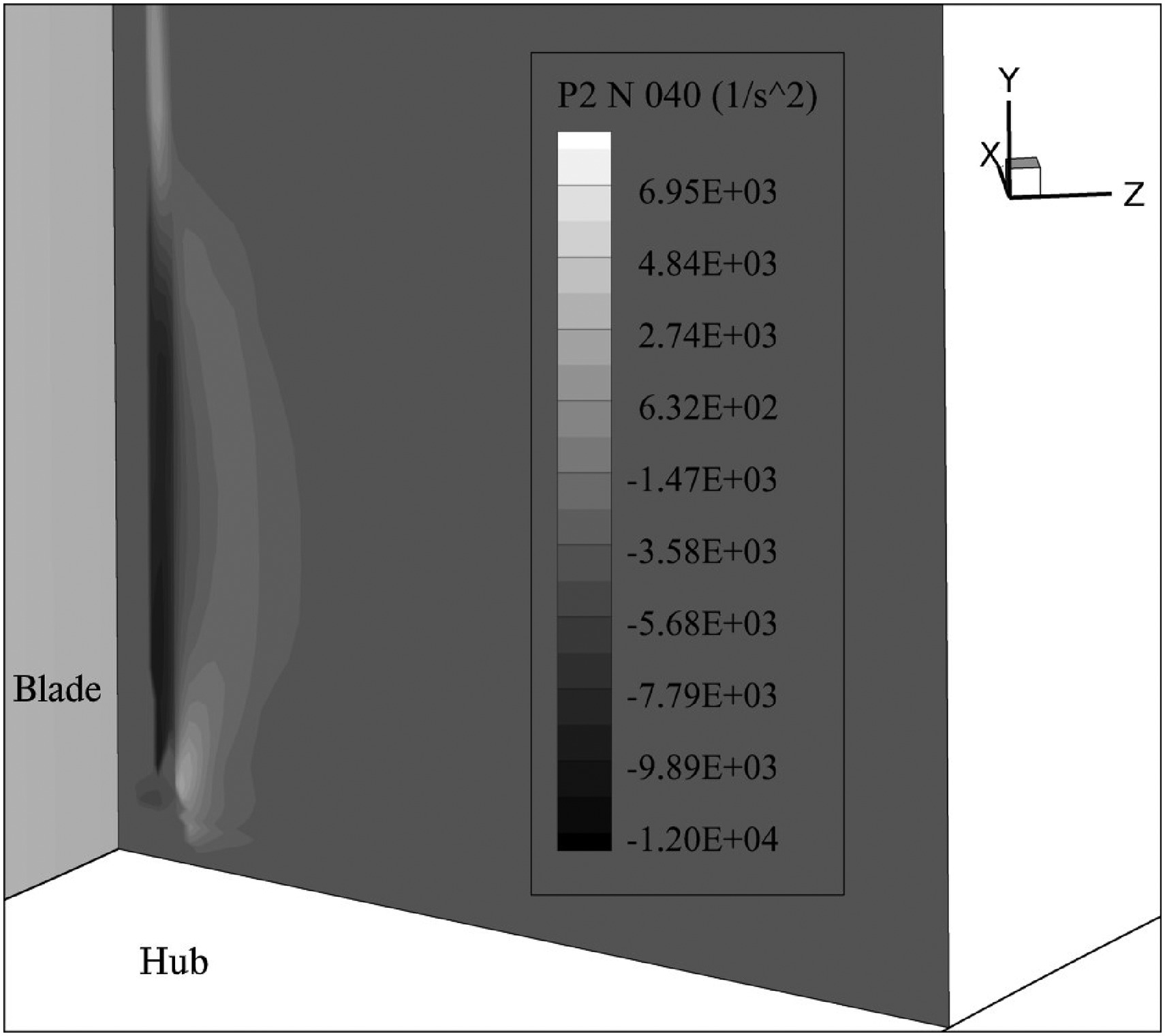

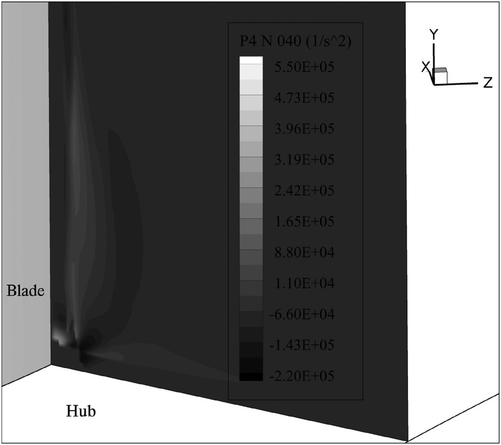
For example, the linear term
Similarly, each component of the Reynolds stress tensor can be split into its linear and quadratic parts. The footnotes 1, 2, 3 in the components of the strain/vorticity tensor denote axial, spanwise and pitchwise directions, respectively.
As seen from Figures 10, 11, 12, and 13, in the corner region just upstream of the origin of separation (see in Figure 9), most of the streamwise vorticity production comes from
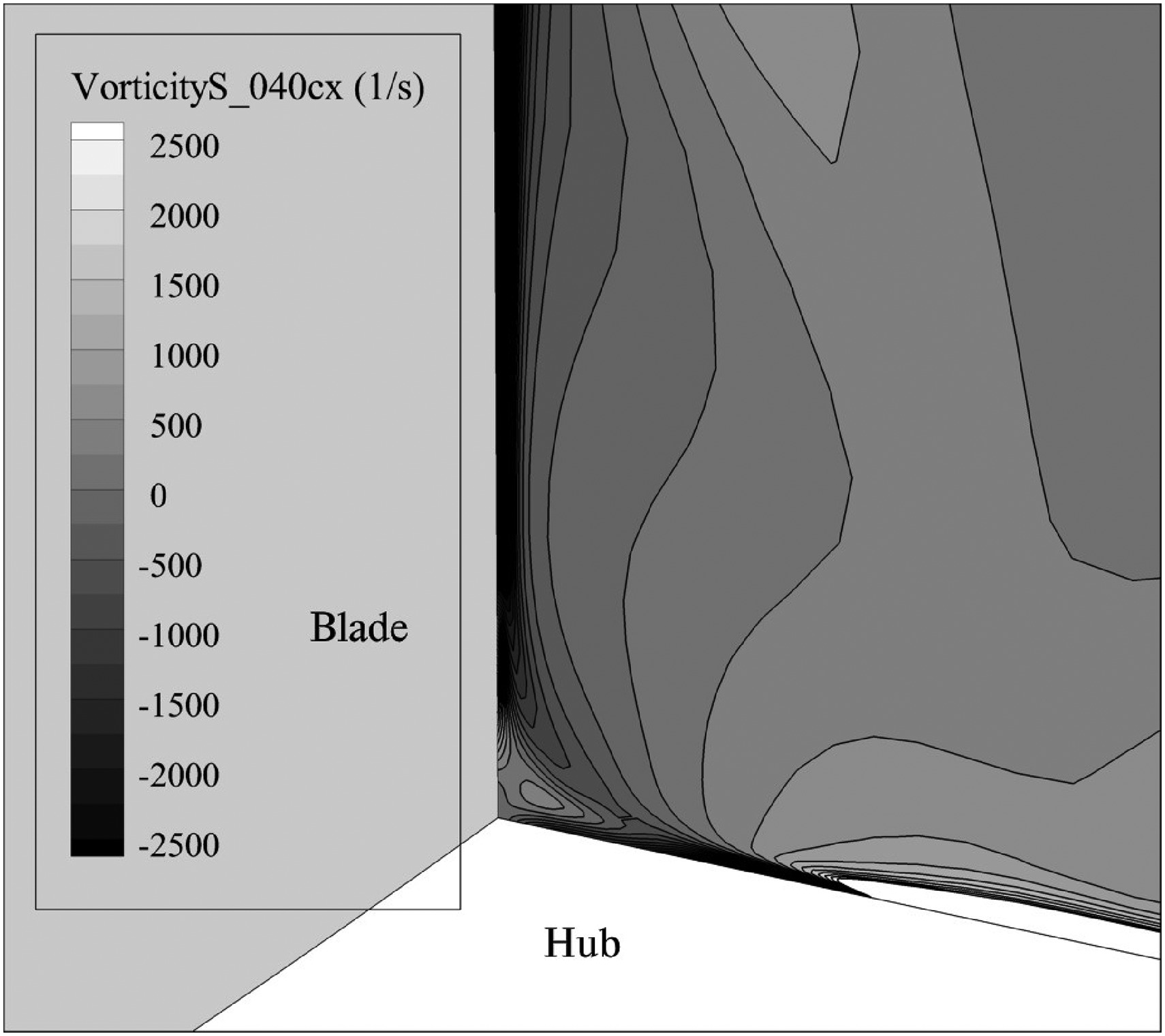
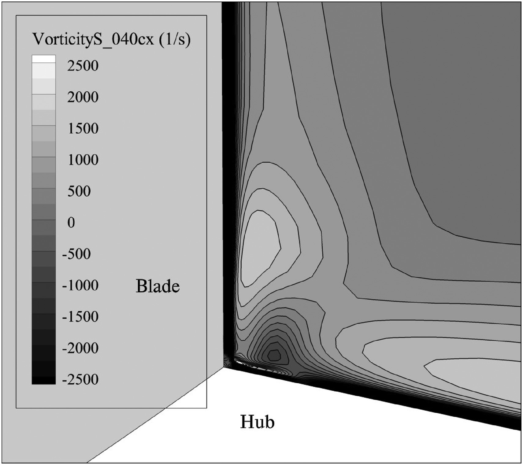
Figures 14 and 15 show the effect of the given anisotropic modification on the streamwise vorticity distribution on the cut plane at
The finding here shows consistency with that from the external flow community (Yamamoto et al., 2012; Mani et al., 2013; Dandois, 2014). In the numerical study of the turbulent square-duct flow (Mani et al., 2013), secondary corner vortices were observed around the corner of the duct by replacement of the Boussinesq closure by the quadratic constitutive relation (Spalart, 2000). The authors claimed that this is attributed to the capability of the quadratic constitutive relation to reproduce the physics of the normal stress anisotropy in the corner region, which leads to the appearance of corner vortices.
Next, the distributions of
Figure 16 shows the selected cut plane, and again it is normal to the blade camber line, i.e.
Figure 16.
Endwall surface friction lines, BSL-2003-NL, i = 0 ∘
Within the corner separation region
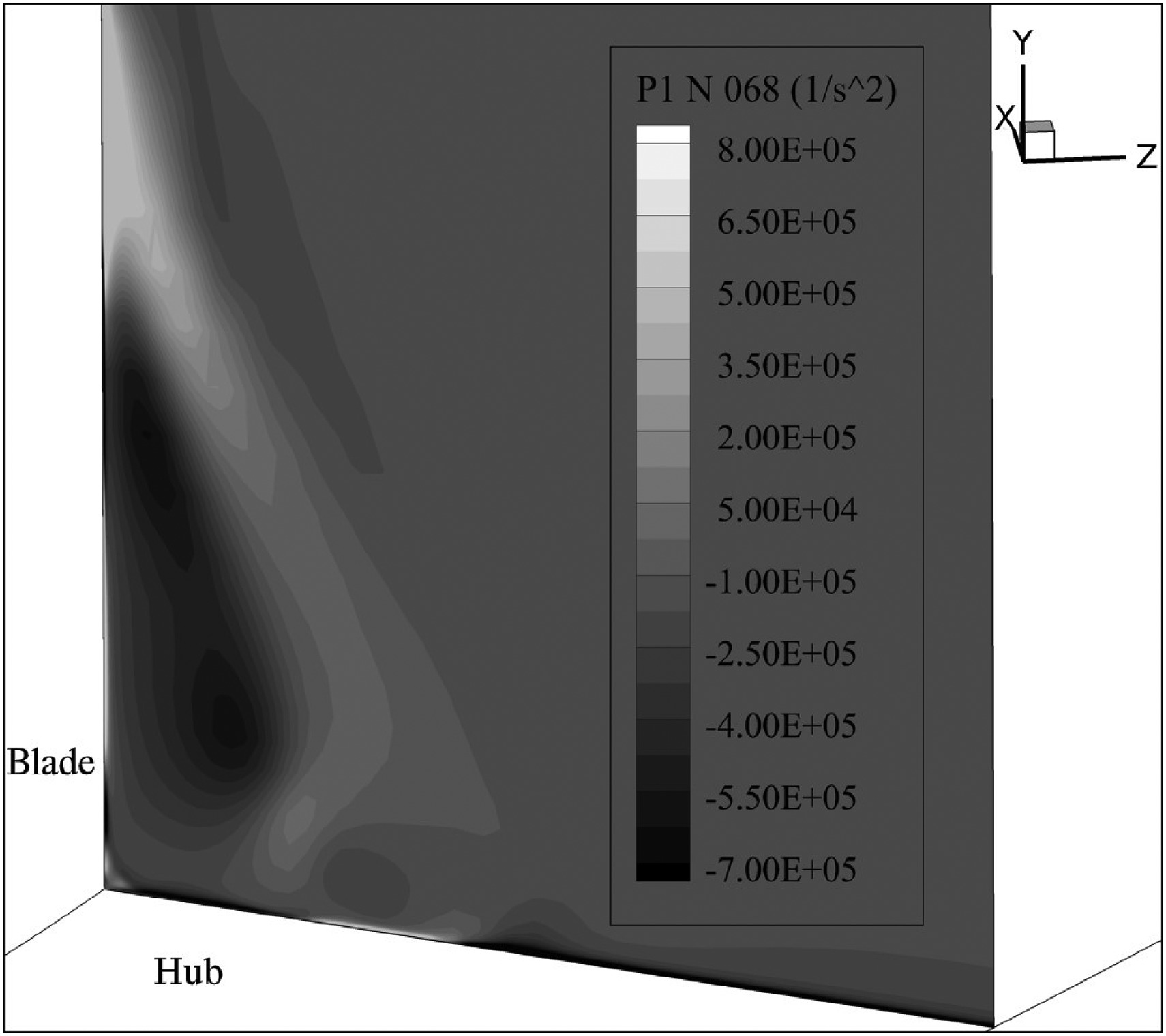

As seen in Figure 17, the contribution of the mean shear skewing to the streamwise vorticity generation mainly concentrates in the separated shear layer between the corner separation region and the main flow where counter-rotating vortices coexist, which enhances the turbulent shear between the corner separation flow and the main passage flow. This contributes to the stronger momentum exchange between the flow outside the separation region and the corner separation flow, energizing the flow inside the corner separation and making it resistant to bulk adverse pressure gradients.
Similar trend can be seen in Figures 19 and 20. The anisotropic modification of the normal stress anisotropy in
In summary, it can be clearly seen that the inclusion of the Reynolds stress anisotropy contributes to the induction of the streamwise vorticities in the corner region. Next, the streamwise vorticity distributions are shown in Figures 21 and 22 to illustrate the effect of the Reynolds stress change on the streamwise vorticity field.

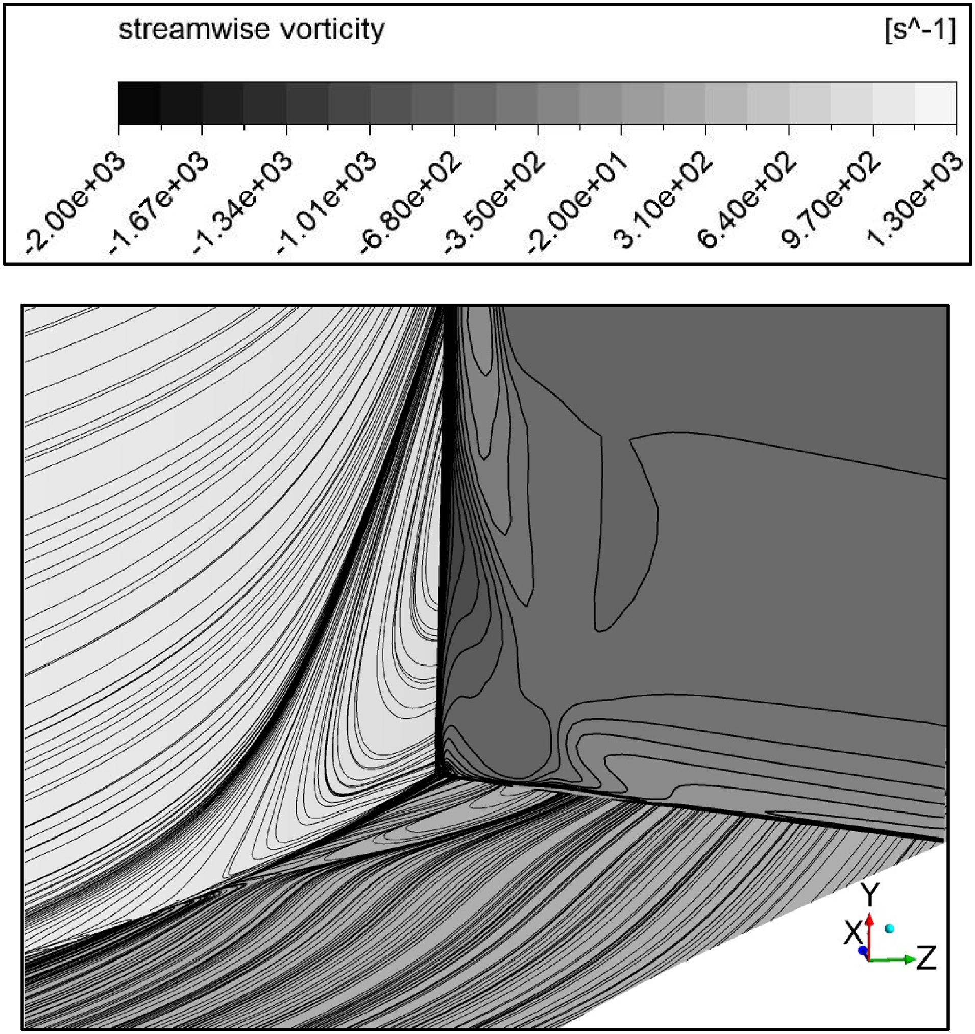
Within the corner separation region, the streamwise vorticity contour lines of BSL-2003-NL concentrate in the separated shear layer between the corner region and the main flow region that are close to the endwall (see in Figure 22). This is consistent with the distribution of the streamwise vorticity source terms
Conclusions
In the present research, a recently proposed quadratic stress-strain constitutive relation based on the
In comparison with the original Boussinesq constitutive relation does, the non-linear, quadratic constitutive relation, when coupled with the Menter's hybrid
One of the physical reasons for the improved predictive capabilities is that the inclusion of the quadratic strain-vorticity term to the Boussinesq Reynolds-stress closure increases the Reynolds stress anisotropy, which contributes to the counter-rotating streamwise vortices being generated in the corner region, and the stronger turbulent shear interaction in the separated shear layer. This in turn leads to more of the higher-momentum fluid in the main passage flow being entrained into the corner region, in which the flow is energized and thus is more resistant to separation.
The engineering analysis of the corner separation flow mainly focuses on the prediction of the blockage due to separation. Considering this, the Menter et al.'s nonlinear explicit RANS turbulence closure shows its strong potential in determining the corner separation size with reasonable accuracy, while maintaining the low cost, numerical robustness, and convenience for implementation.
However, as the inlet flow incidence is increased, the corner separation becomes larger and more complex. More significant discrepancies between the CFD results and the experimental measurements are observed in terms of the blockage. Herein it shall be realized that the effect of the turbulence anisotropy on corner flow structures is characterized by modelling. The modelling uncertainties still exist at off-design flow conditions. This calls for the high-fidelity scale-resolving simulations in order to obtain understandings of the source of the anisotropy based on turbulence resolved simulation results. Further improvement of the Menter et al.'s nonlinear turbulence closure could be carried out based on the insight and understandings gained from further studies of the scale-resolving flow solutions.
Nomenclature
Cps
static pressure coefficient,
i
inlet incidence angle, degree
k
turbulence kinetic energy, m2/s2
local static pressure, Pa
endwall static pressure at inlet, Pa
freestream total pressure at inlet, Pa
freestream turbulence intensity,
wall-friction velocity, m/s
u+
non-dimensional mean velocity,
fluctuating velocity in the axial direction, m/s
freestream velocity at inlet, m/s
kinematic viscosity of the working fluid, m2/s
fluctuating velocity in the spanwise direction, m/s
fluctuating velocity in the pitchwise direction, m/s
y
wall-normal distance, m
y+
non-dimensional wall-normal distance,
rotating angle between the local coordinate system s-y-n and the Cartesian coordinate system x-y-z
Reynolds average of
specific dissipation rate, 1/s