
Introduction
The near casing flow region of an axial compressor has long been a subject of interest due to its potential link to spike stall inception. For a low-speed axial compressor, the tip region is dominated by low momentum fluid due to casing boundary layer effects and the tip leakage flow (TLF). The low momentum fluid results in blockage effects that intensify as the compressor reaches its stability limit. Furukawa et al. (1999) numerically showed that the rapid rise of the blockage region in a low-speed compressor at near stall conditions can be attributed to the breakdown of the tip-leakage vortex (TLV). The abrupt drop in pressure rise across the rotor is explained by the suction side boundary layer separation due to the interaction with the blockage. In another numerical study in a low-speed environment, Hoying et al. (1999) showed that the TLV trajectory of an isolated rotor becomes more aligned to the circumferential direction as the operating point of the compressor moves closer towards stall. This phenomenon can be explained by the axial momentum balance across the rotor. As the mass flow rate is reduced, the pressure rise across the rotor increases. A further reduction in mass flow rate results in reduced axial flow momentum and a stronger pressure rise. This imbalance pushes the TLV trajectory upstream and causes a “spill forward” effect.
The “spill forward” effect can be mitigated by using circumferential casing grooves. An axial momentum analysis by Shabbir and Adamczyk (2005) showed that the stall margin improvement (SMI) by circumferential grooves is due to the radial transport of axial momentum across the grooves. In the axial momentum balance equation, the radial transport of axial momentum at the groove-main flow interface adds a positive term that helps to balance the axial pressure force across the rotor. This delays the “spill forward” that is thought to be responsible for the stall. Houghton and Day (2009) studied the effect of axial variation of the location of a single circumferential groove in a low-speed compressor. They considered a shallow groove and a deep groove for this. For both type of grooves there were two axial locations that produced the best SMI, at 10% and 50% axial chord
These questions can only be answered if a design optimisation study is performed. However, a design optimisation study would not address the disadvantage of the “black-box” approach explained earlier if the SMI itself is chosen as the objective function. This is because the optimiser algorithm has no knowledge about the inner workings of the groove that produces the highest SMI. The aim of this paper, therefore, is to show that a circumferential groove design can be obtained through a “physics-based optimisation” approach where a blockage parameter is chosen as one of the objective functions. The choice of the blockage parameter is explained in the first part of this paper. Next, the implementation of the blockage-based optimisation approach to obtain a single circumferential groove is presented. Lastly, the SMI and flow features of the optimised casing groove with respect to smooth casing are shown.
Computational method
Numerical domain and grid
The numerical domain and the grid used for this study are shown in Figure 1. The numerical domain is based on an isolated low-speed axial compressor (LSAC) rotor. The rotor blade of the LSAC is obtained through an inverse-design method using MISES (Youngren and Drela, 2008). The inverse design method is an iterative method used to obtain a desired blade shape from a prescribed blade loading. The aim of the inverse-design method is to obtain a tip-critical compressor rotor that is suitable for passive casing treatment study. Hence, the prescribed blade loading is obtained numerically from an axial compressor that is known to exhibit a spike-stall inception pattern. The 3D rotor blade is generated by radially stacking seven 2D profiles at as many spanwise positions. The hub and casing are parallel to one another resulting in a constant annulus height across the blade. The 3D blade design has a nearly constant exit flow angle (absolute) distribution in the spanwise direction. This agrees with the flow angle distribution of the tip critical compressor of which the inverse design is attempted. Aerodynamic design parameters of the LSAC are presented in Table 1.
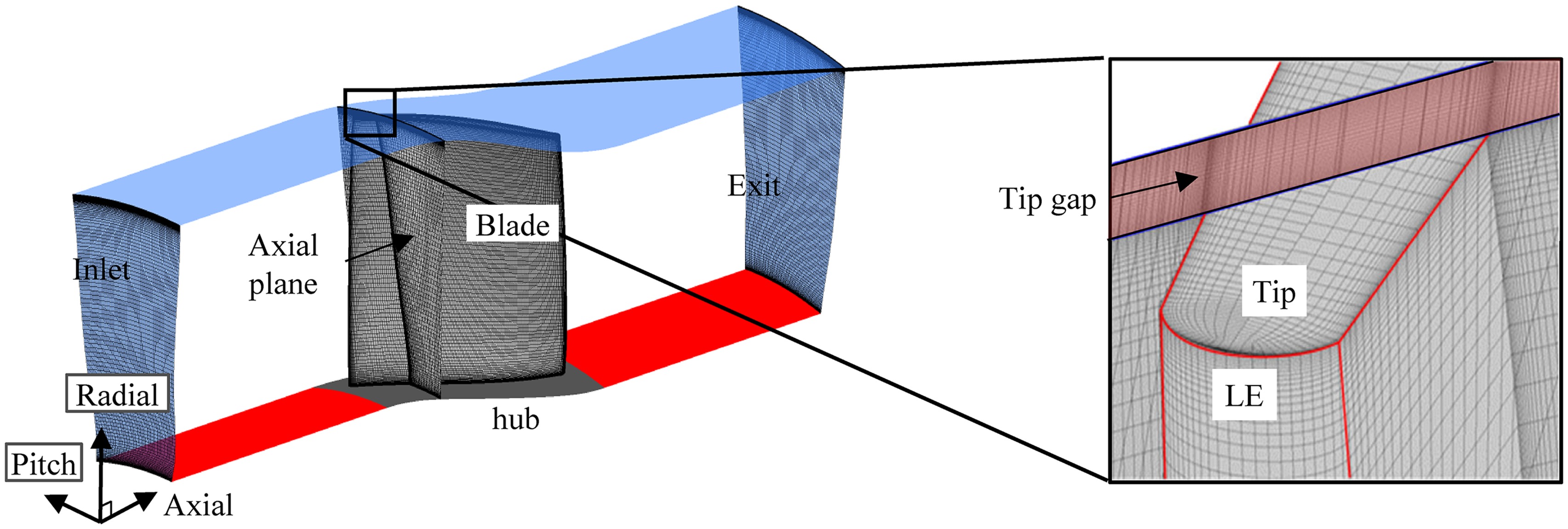
Table 1.
Aerodynamic properties of LSAC.
The single passage numerical domain and unstructured grid are generated automatically using ANSYS Turbogrid 17.1. The grids are generated by setting the target passage grid node count and the boundary layer grid node count near the walls. A grid independence study was conducted by varying the total number of elements, but with a fixed y+ value (≈2). The change in the converged mass flow rate value and the blade surface static pressure distribution at 98% span was found to be negligible for grid resolutions that are finer. The resulting blade domain has a total grid count of 3.2 million. This is made up of 143 elements in the spanwise direction (of which 30 are in the tip gap region), 72 elements in the circumferential direction and 310 elements in the chordwise direction (of which 147 are within the blade passage). Boundary layer meshing is used in the near wall regions over the blade surfaces (typically 30 layers normal to the blade) and the end wall surfaces.
Numerical setup and boundary conditions
The 3D steady RANS equations are solved using ANSYS CFX 17.1 code. The code uses a cell-centred finite volume approach to evaluate the numerical fluxes. Flux values at the cell-boundary are obtained using a high-resolution upwind scheme (ANSYS CFX Theory Guide, 2016). The high-resolution upwind scheme is a blended scheme that addresses the shortcomings of the first and second order upwind schemes. The flow is assumed to be fully turbulent and the standard
At the inlet, the total pressure and total temperature profiles are prescribed. The steady calculation uses an inlet turbulence intensity of 5% along with an eddy viscosity ratio of 10. The total pressure profile used at the inlet boundary corresponds to that of a turbulent boundary layer with a displacement thickness of approximately 5% of the annulus height. A radial equilibrium exit static pressure condition is imposed at the outlet. Flow within the whole domain is solved in the rotating frame of reference, and all stationary walls are set to be counter-rotating. All walls are treated as smooth and adiabatic. The convergence rate is accelerated using an algebraic multi-grid (AMG) approach built into the solver.
Smooth casing results and discussion
Performance characteristics
The performance characteristics of the LSAC for the smooth casing case are shown in Figure 2. The abscissa of Figure 2 is the flow coefficient,
Figure 2.
Performance characteristics of the LSAC. (a) Total-static pressure rise coefficient and (b) Isen-tropic efficiency.
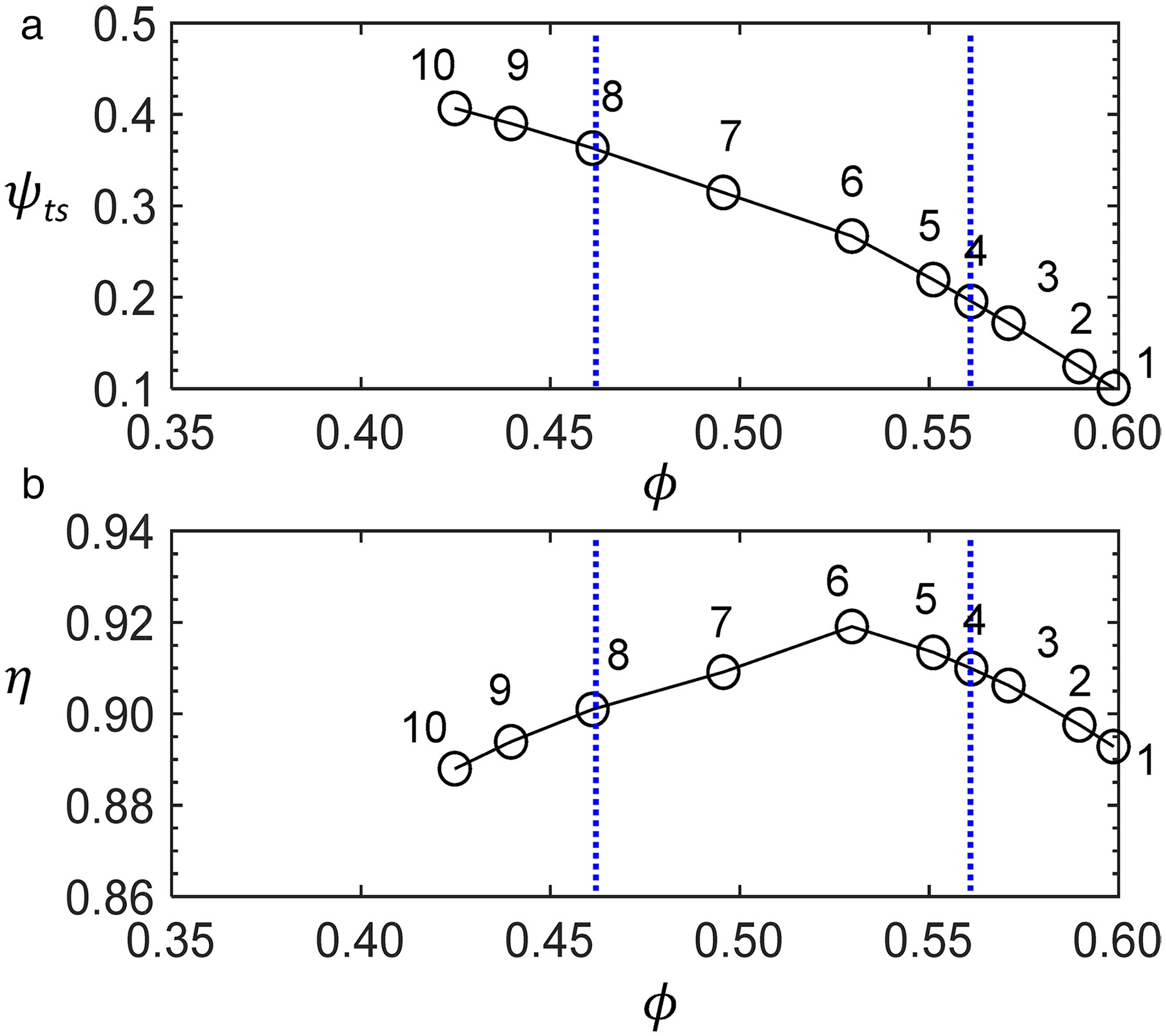
Operating point 1, in Figure 2, corresponds to a hub exit static pressure of 101,350 Pa. The characteristic is obtained by gradually increasing the hub static pressure by a value between 50–100 Pa. Operating point 4 and 8 represent the conditions at near design and near stall respectively. The last stable operating point (Operating point 10) is determined iteratively using a “bisection method” type approach. Here, the size of the hub static pressure increment is updated until any further increase of 5 Pa fails to produce a converged solution. The convergence criteria set for all simulations are as following:
The calculations are run for a minimum of 2000 iterations.
Coefficient of variation (CV) of the inlet mass flow rate value must not exceed 0.001 for the last 200 iterations. (CV is the ratio between the standard deviation to the mean.)
The residuals of mass momentum and energy for the last 1,000 iterations fall below an acceptable value (typically 10−5) or remain stable below this low value.
The computational methodology as used here has been extensively validated in Mustaffa and Kanjirakkad (2019, 2020).
Tip region flow
As shown in Figure 2a, the stability limit occurs before the
Figure 3.
Normalised axial velocity contour plotted for an axial plane located at 0.04 c_(ax,t) at operating point 8.
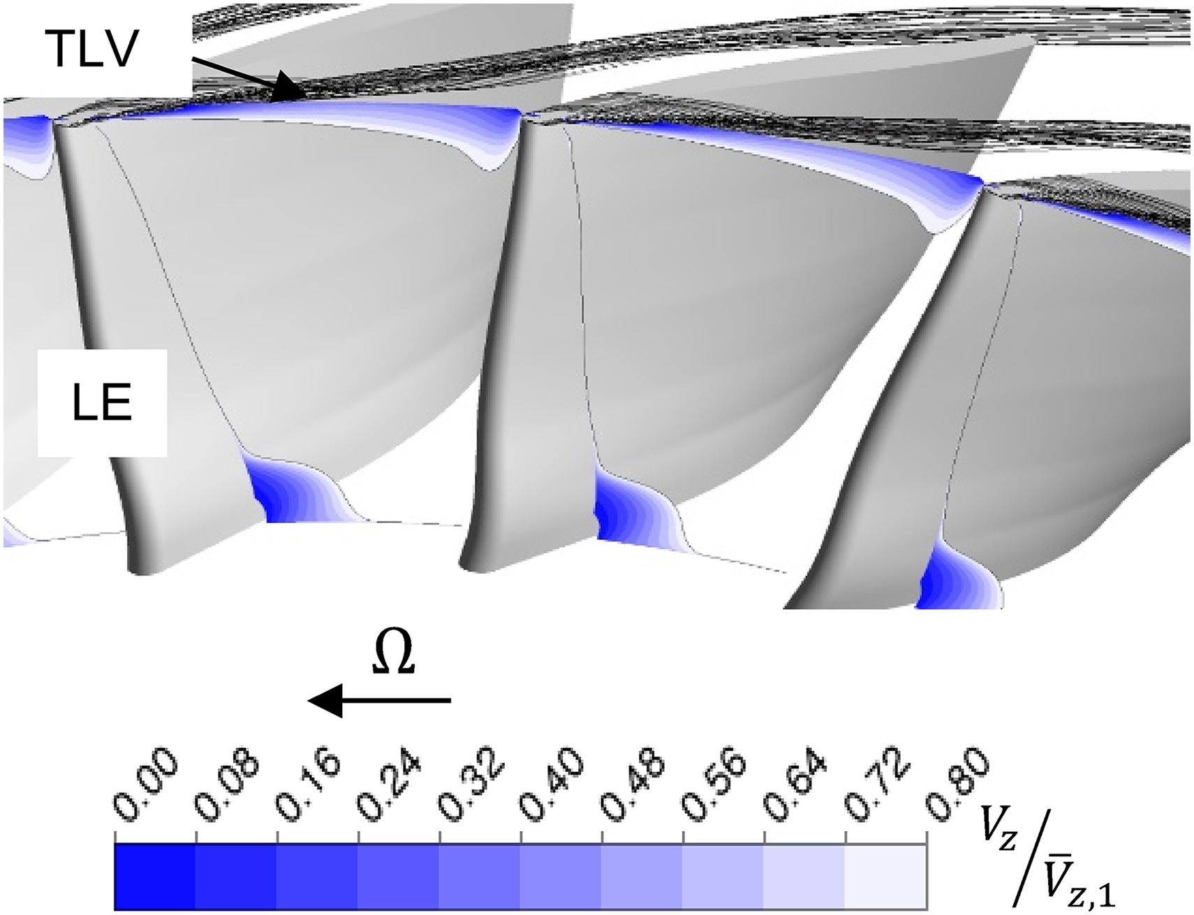
The build-up of blockage near the casing as the compressor approaches stall can be investigated by plotting the normalised axial velocity contour inside the tip gap for operating point 4 (near design) and 8 (near stall) as shown in Figure 4. In comparison to operating point 4, the blockage region due to the TLF at operating point 8 occupies a relatively larger portion of tip gap region within the blade passage. This is expected since the TLF is pressure-driven such that at a lower
Figure 4.
Normalised axial velocity contour inside the tip gap (50% of tip gap height, τ) for (a) operating point 4 and (b) operating point 8.
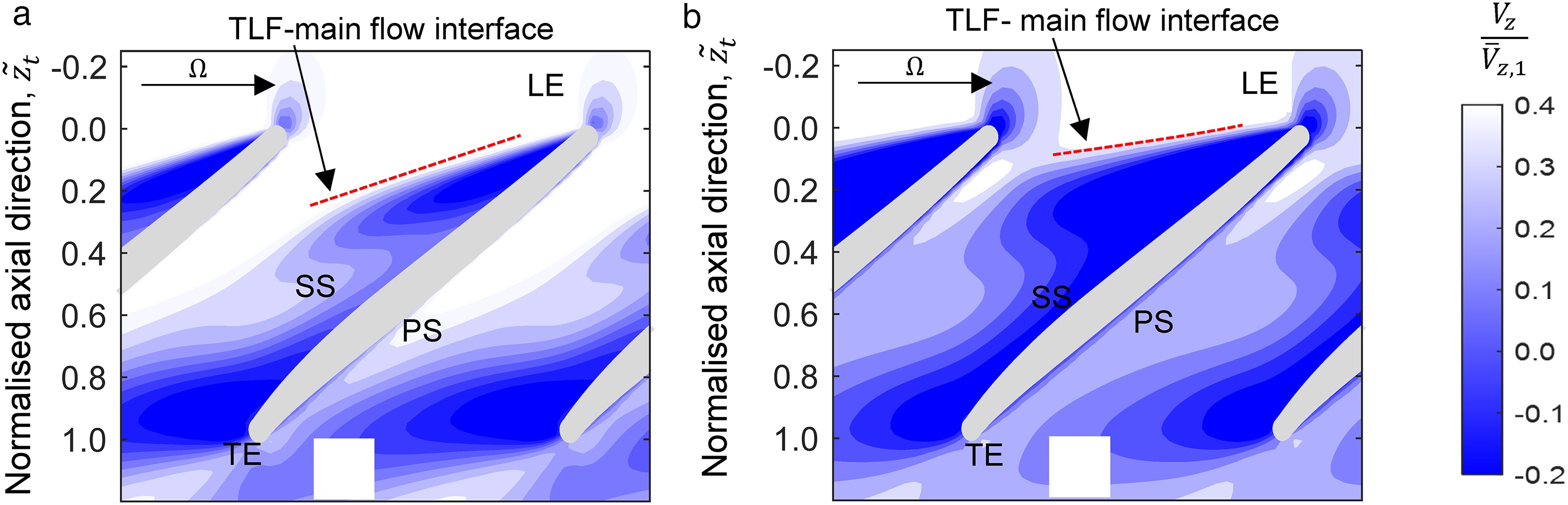
In addition, at operating point 8, it can be seen that the interface of the TLF and the incoming flow is more aligned to the circumferential direction compared to operating point 4. This is similar to what has been described in Hoying et al. (1999) where, at near stall conditions, it is found that the upstream movement of the TLV eventually leads to a “spill forward” effect. The blockage near the blade LE of the suction side (SS) is likely to be caused by a stronger TLV and the increased TLF. The TLV trajectory can be found by extracting the normalised static pressure profiles along several constant pitch lines as shown in Figure 5.
Figure 5.
TLV trajectory (red line) extracted from static pressure contour at mid tip gap at operating point 4.
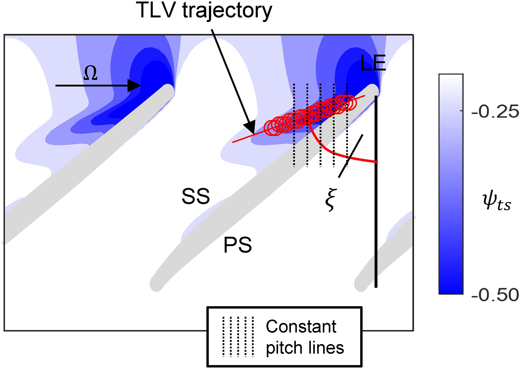
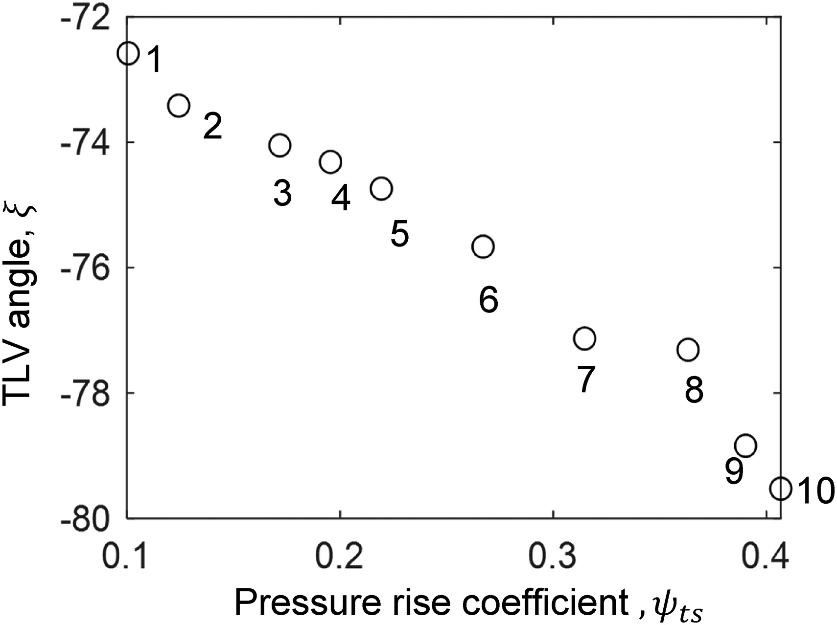
For each constant pitch line, the axial coordinate of the minimum static pressure is found through interpolation. The trajectory of the TLV can be found through linear fitting. The slope of the TLV trajectories is represented as TLV angle,
Tip leakage momentum
As mentioned earlier, the increased loading near the blade tip LE at conditions close to stall, contributes to the increase of the TLF pitch-wise velocity component which, in turn, appears as blockage due to reduction in the axial velocity component. The strength of the TLF that also affects the strength of the TLV can be quantified by calculating the TLF momentum inside the tip gap region as shown in Equation 3.
Here,

Quantification of near casing blockage
The preceding discussion has shown that the upstream movement of the TLF-main flow interface can be linked to the increased blockage (axial velocity deficit) regions at conditions near stall. It is, therefore, thought to be a worthwhile exercise to quantify this blockage to further explore its link to the initiation of stall. The blockage quantification method is based on a mass flow overshoot method introduced by Sakuma et al. (2013) in order to identify and visualise “blocked” cells in an axial plane. Blocked cells are identified by sorting and summing the mass flow of each grid cell in that plane in a descending order. If cells with negative axial velocity (flow reversal) values exist, the sum of all positive axial velocity will overshoot the inlet mass flow value. The summation is stopped when the summed mass flow reaches the inlet mass flow value. Cells that are yet to be summed are considered as “blocked” and are assigned a binary blockage index
Figure 8.
Location of the “blocked” cells at an axial plane location same as in Figure 3 at operating point 8 (looked from the front).

Based on the overshoot method described above, a non- dimensional blockage parameter,
Here, N is the total number of cells in the plane.
Figure 9 shows the distribution of
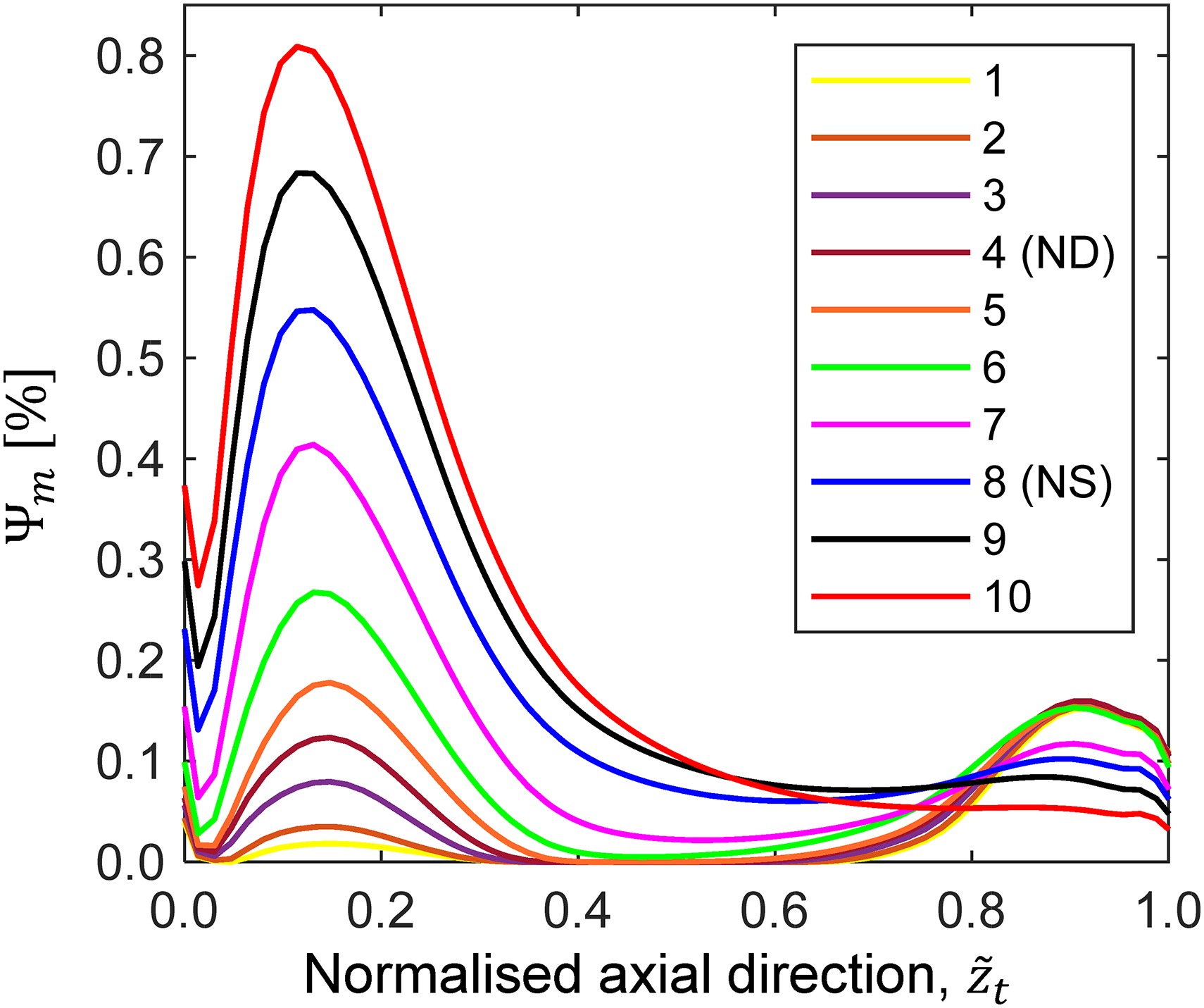
Near the TE
Circumferential groove results and discussion
The blockage quantification method has established the link between blockage and the inception of rotating stall. Based on this, a design optimisation method to obtain a single circumferential groove is attempted. The objective of the optimisation is to find a single groove design that minimises the peak blockage with the least efficiency penalty. A method that couples a surrogate modelling technique to a multi-objective evolutionary algorithm is employed. The primary aim of using the surrogate model is to reduce the computational cost associated with high fidelity CFD simulations. The surrogate model used is a supervised-learning tree-based algorithm (Breiman, 2001) called Random Forest (RF). RF is an ensemble of decision trees that can be used for predicting the response of continuous variables. The RF is constructed from input and output training data. The input training data is generated using a space-filling design sampling technique called Latin Hypercube Sampling (LHS). First, the groove design is parameterised to define the shape of the groove using four variables that are described later in Figure 10a. The shape of the groove is obtained by sampling 100 datasets across a predefined design space boundary. The LHS technique ensures that population of groove shapes generated covers the whole spectrum of the design space. The output data are obtained through CFD simulation of the 100 groove shapes at a single operating condition corresponding to operating point 8 in Figure 2a which represents the near-stall condition. The peak blockage and efficiency of each groove test case is interrogated. The optimisation algorithm implemented is a Multi-Objective Genetic Algorithm (MOGA). The optimiser performs a random search method and outputs a set of groove designs that are Pareto-optimal solutions. The set of groove designs from the Pareto-optimal solution are verified through CFD. The best case is chosen to be the groove design that numerically stalls at the lowest flow coefficient using the previously mentioned convergence criteria. Further details regarding the surrogate-based optimisation technique can be found in Mustaffa and Kanjirakkad (2019, 2020) where a similar approach was applied to an isolated transonic rotor.
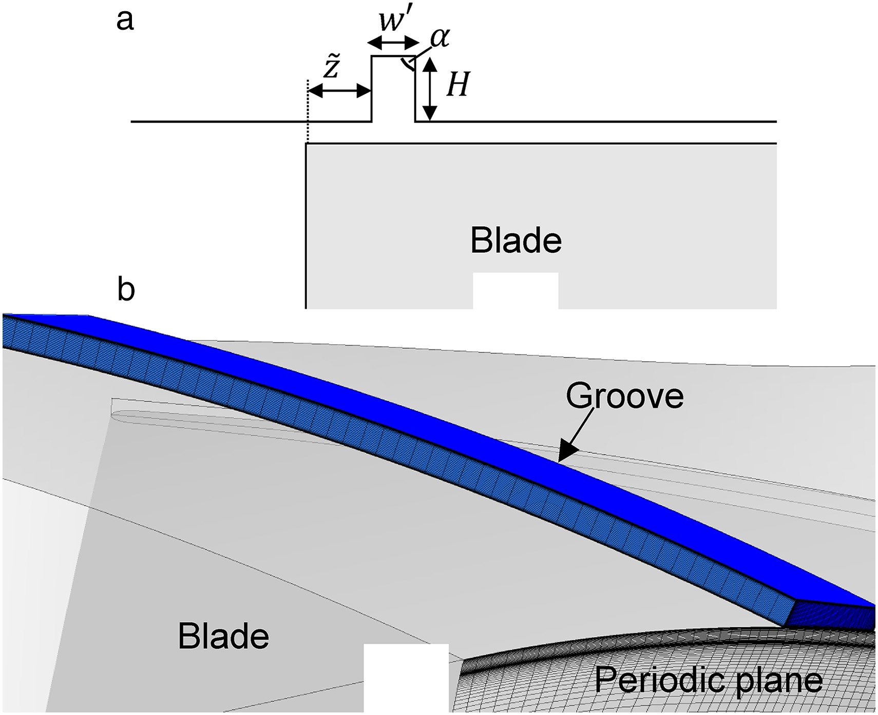
The optimal single groove solution is obtained as parameters
Figure 11 shows the characteristic of the rotor with the grooved casing in comparison to the one with smooth casing. The SMI
Figure 11.
Performance characteristic comparison of the optimised groove and the smooth casing. (a) Pressure rise coefficient and (b) isentropic efficiency.
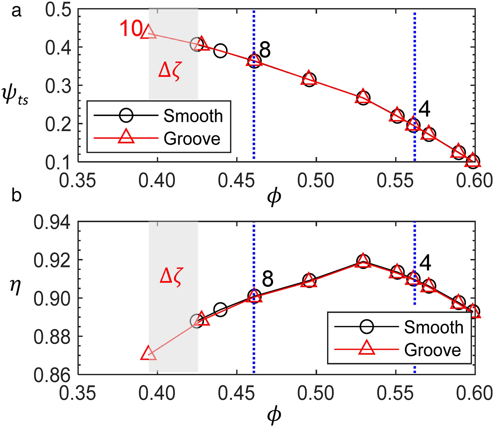
Here, as before,
Figure 12 shows the normalised axial velocity contour in the mid-tip-gap for the grooved casing. Here, the TLF-main flow interface (dotted red line) of the grooved casing is shifted further towards the blade suction side than that for the smooth casing shown in Figure 4b. This delays the “spill forward” effect and hence results in an improved stall margin.
Figure 12.
Normalised axial velocity contour inside the tip gap (50% of tip gap height, τ) for the grooved casing at operating point 8.
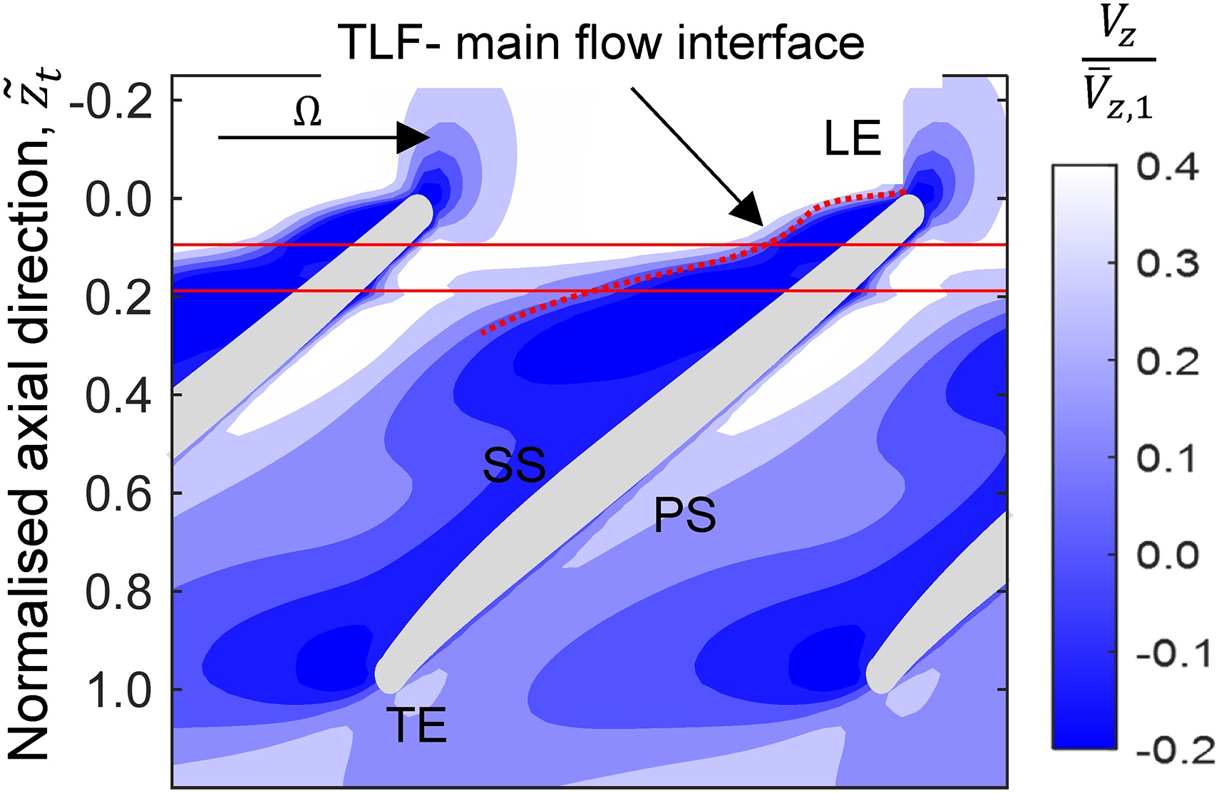
Figure 13 shows the comparison of the non-dimensional blockage parameter,
Figure 13.
Comparison of the grooved casing blockage parameter, Ψ_m, at operating point 8 with respect to the smooth casing.

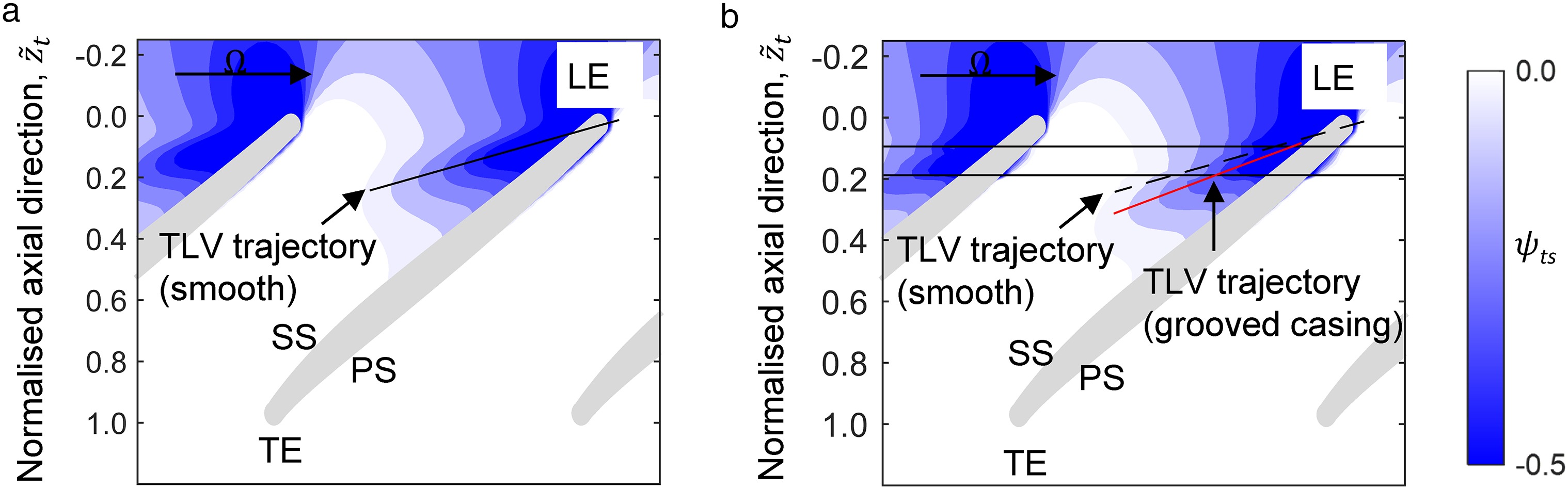
Figure 14 shows the non-dimensional casing static pressure contours with the blade tip profile made visible for clarity. Figure 14a shows the contours for the smooth casing at near stall operating point (operating point 8.). The tip vortex trajectory obtained by tracking the trough of the static pressure profile is overlaid on top of the contour map. Figure 14b shows the same contours for the grooved casing. The red line shows the trajectory of the tip leakage vortex developing downstream of the LE of the groove. A dotted line is also shown that represents the trajectory of the smooth casing as before. Clearly, the interaction of the tip vortex with the groove has resulted in a reduced TLV angle. Using the method as described in relation to Figure 5 this reduction in angle is estimated to be 2.7°. This is significant given that TLV angle shift from operating point 4 to operating point 8 is only about 4° as described earlier. Researchers such as Sakuma et al. (2013) have attributed such a shift in TLV to SMI in a transonic compressor. However, the study by Houghton and Day (2009) in a low-speed compressor concluded that TLV modification was not necessary for achieving SMI. But it remains a fact, even in the study by Houghton and Day (2009), that grooves that are positioned downstream of the TLV origin, but closer to the LE do show a modification of the TLV trajectory. This further points to the fact that the positioning of the groove in relation to the peak blockage as implemented in the present study is key to achieving maximum SMI with least efficiency penalty. However, none of the SMI studies as previously mentioned have quantified the blockage inside passage near the tip region and linked it to the improved stall margin that they have reported.
Figure 14.
Non-dimensional casing static pressure contour for (a) operating point 4 and (b) operating point 8.
The strategy to quantify the blockage near the casing using a non-dimensional parameter and to use this parameter to obtain a circumferential casing groove that provides improved SMI through an optimisation process has therefore been shown to be successful. This method has already been shown numerically to be useful for improving the stall margin in a transonic compressor rotor by Mustaffa and Kanjirakkad (2019, 2020). The flow physics associated with blockage and stall is very different in the transonic environment that is dominated by passage shock and its interaction with the TLV. The outcome of the present study in a low-speed compressor rotor therefore offers the confidence that the physics-based optimisation approach adopted here for achieving SMI is a robust one.
Conclusions
The near casing flow region of a tip-critical low speed axial compressor (LSAC) rotor has been studied numerically. The blockage in the tip region is quantified using a mass flow based non-dimensional parameter. Improvement of stall margin is attempted using an optimised casing groove geometry using a physics-based approach that minimises the peak tip blockage as evaluated using the above parameter. The conclusions are summarised as the following:
At conditions close to stall, the blade loading increases due to the increased back pressure. This results in a stronger TLV and TLF. By tracking the TLV trajectory (approximated as the locus of static pressure minima) it is observed that the TLV angle increases by about 4° from near design to the near stall operating point. This increase in TLV angle contributes to the upstream movement of the TLF-main flow interface.
The strength of the TLF is evaluated by calculating the tip leakage momentum across the tip. At conditions close to stall, it is found that the TLF momentum increases near the LE edge region. The TLF also contributes to the upstream movement of the TLF-main flow interface and the increase of the TLV angle
The near casing blockage region is quantified using a mass flow-based blockage parameter
Based on the blockage analysis performed on the smooth casing, a design optimisation is attempted to obtain a single circumferential groove that reduces the peak blockage with least efficiency penalty. The optimised single groove results in a SMI of 5.4%. The SMI by the groove is shown to be a result of the reduction of the peak blockage magnitude and a shift in the TLV angle. Both factors result in delaying the upstream movement of the TLF-main flow interface.
The identification of the location and the minimisation of the peak of the tip blockage by appropriately positioning the groove is therefore recommended as a possible route for designers to achieve SMI through casing modification.
Nomenclature
Annulus area
Groove height
Tip leakage flow momentum
Static, Total pressure
Blade speed at mid-span
Velocity
Averaged value of variable
Mid-span value of variable
Normal component to blade chord
Tip axial chord
Mass flow rate
Groove width
Axial direction
Groove axial position
Stage loading coefficient,
Non-dimensional blockage parameter
Blade RPM
Groove upper internal angle
Stall margin, stall margin improvement
Isentropic efficiency
TLV angle
Density
Flow coefficient,
Blockage parameter
Total-static pressure rise coefficient
TLV
Tip leakage vortex
TLF
Tip leakage flow
1, 2
Refers to rotor inlet and exit conditions respectively