Introduction

The expansion of steam in a low-pressure steam turbine leads to the saturation line being crossed and thus to the formation of wetness. Wet steam is inseparably associated with the degradation of the efficiency as well as increased rates of erosion caused by droplets contained in the two-phase flow.

Wetness losses have been comprehensively investigated in the past and it is now widely recognized that the main wetness losses can be categorized into three groups. (1) Thermodynamic relaxation is caused by rapid expansion of the steam into a meta-stable non-equilibrium state allowing for sub-cooling, followed by an irreversible heat exchange as first droplets are created by nucleation. (2) Kinematic relaxation results from friction between the liquid and the vapour phase. (3) Braking losses are generated by large droplets which impinge on the surfaces of moving blades and thus reduce the amount of work. (Gyarmathy, 1962; Kreitmeier et al., 2005; Kawagishi et al., 2013; Starzmann et al., 2014; Wu et al., 2017).

The phenomenon of water droplet erosion is usually described with successively occurring phases. Tiny droplets are created as the sub-cooled steam returns to a state of equilibrium (homogenous nucleation). This primary fog initially exhibits a small inertia and is thus able to follow the vapour phase into the downstream blade passages. However, increasing velocity slip between the phases and other mechanisms (Senoo and White, 2017) allow the primary fog to deposit on vane and blade surfaces to form a liquid water film. Driven by the shear of the surrounding vapour phase, gravity (stationary vanes) and centrifugal force (rotating blades), the film flows towards the trailing edge where eventually droplets are shed. Those secondary droplets are larger and exhibit a substantial velocity slip (Schuerhoff et al., 2015). The relatively large impact velocities of those droplets on the surfaces of rotating blades can cause severe erosion damage. In addition to the impact velocity, further parameters are found to affect the erosion rate such as the impact angle, droplet size, number of droplets and the hardness of material. The correlation of those parameters to the erosion rate is investigated numerically (Han et al., 2012) and experimentally (Ahmad et al., 2013). Further work was carried out to derive a model for the erosion rate from the named parameters (Lee et al., 2003).

In order to reduce the severity of the erosion damage several measures are taken which can be divided into “active measures” and “passive measures”.

Active measures primarily serve to reduce the amount of secondary droplets in the flow by e.g. annular suction slots in casing walls, extraction slots on the airfoil surface of guide vanes, heated stationary vanes or injection of hot steam through the trailing edges to evaporate secondary droplets in the wake of the trailing edge (Xu et al., 2008). Also increased axial spacing between vanes and blades to reduce velocity slip can be assigned to active measures (Schuerhoff et al., 2015). Particularly the application of extraction / suction slots has been in focus of numerical and experimental investigations in the last decades. (Wang et al., 2009; Gribin et al., 2015; Li et al., 2018; Hoznedl et al., 2019).

Passive measures however aim at increasing the erosion resistance of the blading by either applying better materials with increased hardness (Lee et al., 2003), flame/laser hardening of leading edges (Yao et al., 2010; Schuerhoff et al., 2015) or by shielding the affected areas with materials such as stellite. Also the application of coatings either for protection or for fog rejection purposes is investigated (Walsh et al., 1993; Buehlmann et al., 2018).

In this paper further work is devoted to the investigation of extraction slots. The performance of an extraction slot is analysed numerically and experimentally in order to gain a better understanding in the predominant effects as well as to assess the suitability of modern numerical methods for the analysis of such application.

Experimental setup

The schematic of the experimental apparatus is shown in Figure 1. The experiment consists of a flat plate, which is located within an open container and exposed to a surrounding air flow. At the leading edge of the flat plate numerous holes are arranged and connected to a water supply system in order to provide for a liquid film. Further downstream, the flat plate is equipped with a water film sensor, which consists of three electrodes (located on the plate) to measure the water film velocity by analysing the electrical resistance between two electrodes and evaluating the time lag. Hence, the water film thickness is not a measured parameter within the experimental setup – it’s recalculated using the measured water film velocity and the predefined supply water mass flow rate. Besides, the flat plate provides for an extraction slot whose performance is investigated within this experiment and a water collection area at the downstream end of the flat plate where the remaining water is collected. Through the suction slot both air and water are extracted from the plate and separated subsequently. The water collected from the extraction slot as well as from the collection area at the downstream end will be measured and compared with the water mass introduced via the supply holes in order to derive the collection rate which is one of the main performance values of such extraction slot.

Figure 1.

Left: Schematic of the experimental apparatus; Right: Photographs of the experimental apparatus.

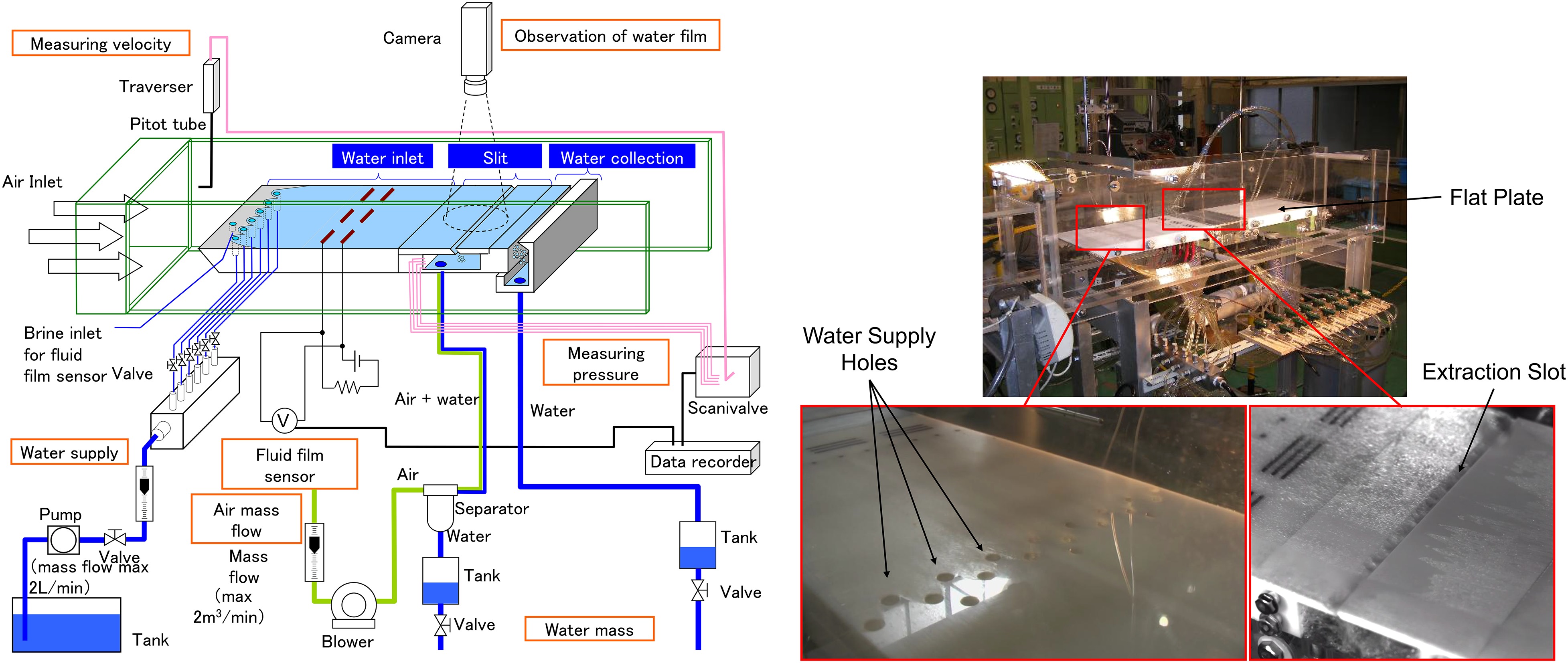
The applied pressure sensors within the measurement have accuracy equal to ±0.06% at full scale (F.S; F.S. 17.2 kPa). For velocity measurement a pitot tube is utilized.

The right hand side of Figure 1 shows two close-up photographs of the flat plate in the vicinity of the water supply holes and the suction slot, respectively.

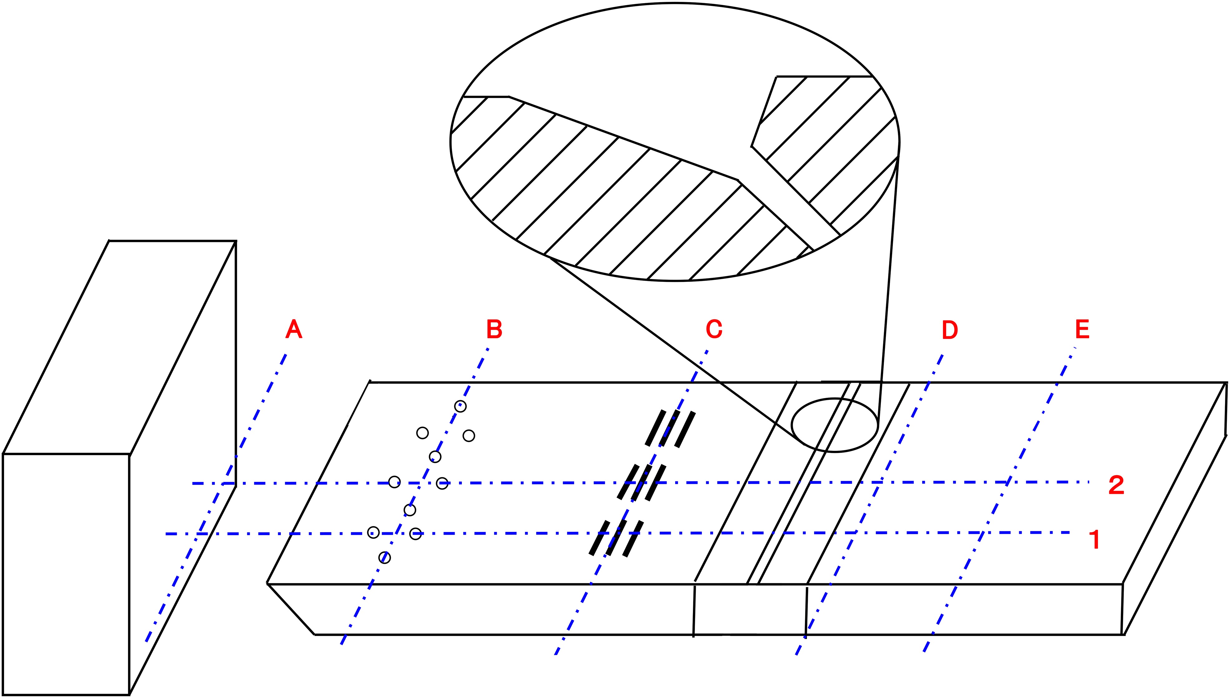
The general geometry of the flat plate as well as the shape of the suction slot’s cross-section is shown in Figure 2. The geometry of the slot is mainly comprised of two angular sloped surfaces on the upstream part of the slot and a blunt edge on the downstream part. Furthermore, the location of measurement planes is highlighted in the figure.

Figure 2.

Positions of evaluation planes and characteristic slot geometry.

On the experimental apparatus described above several cases have been performed in order to assess the dependency of the slot’s performance from different parameters. The main influencing factors are the water mass flow rate and the velocity of the surrounding air. As can be derived from Table 1 four cases have been investigated for this study with variation of the air velocity as well as the water flow rate.

Numerical setup and theory

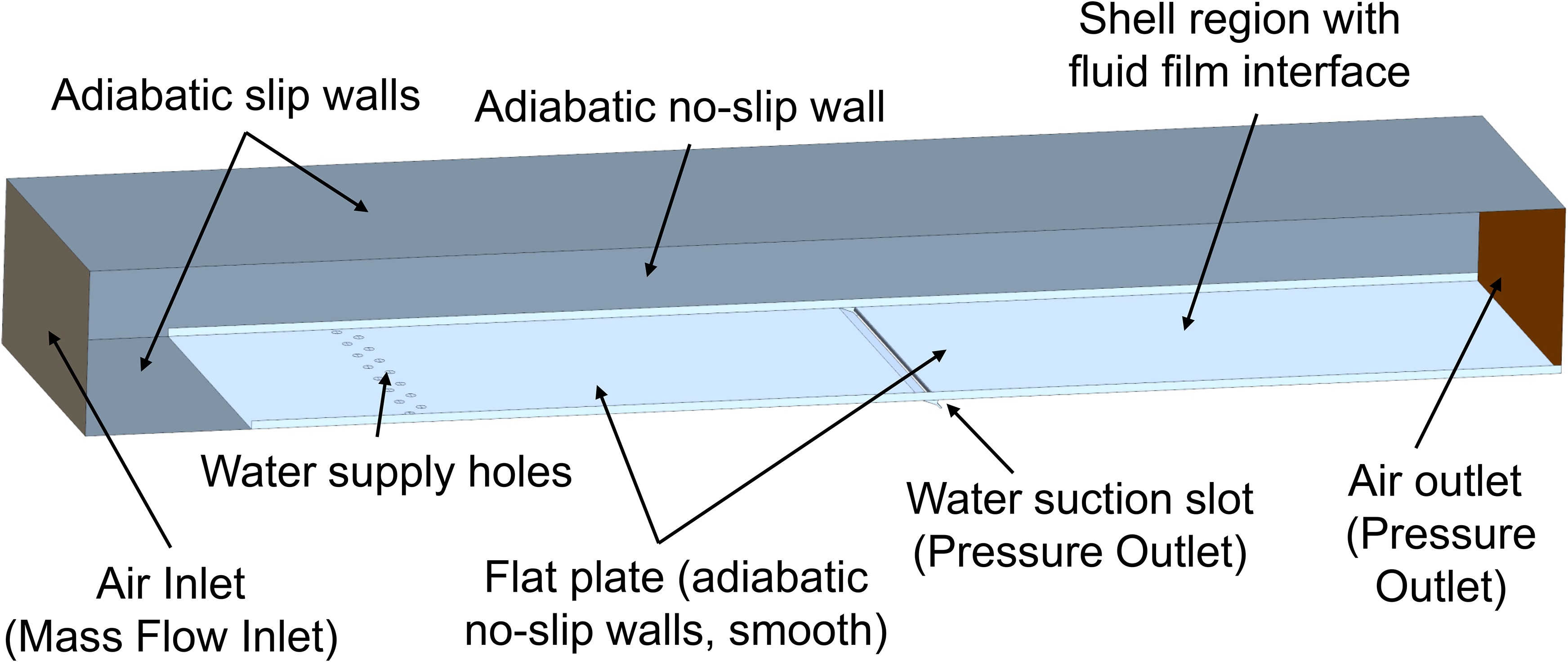
The main features of the test-rig are applied to model the simulation domain for the numerical analyses (cf. Figure 3). Further features such as the water collection region at the downstream end of the flat plate are omitted from the simulation domain after a sensitivity analysis showed negligible impact on the results.

Figure 3.

Overview of numerical domain considered in CFD simulations.

Unsteady multiphase CFD simulations in the commercial Multiphysics CFD solver STAR-CCM+ (version 13.06) under application of a Film-Eulerian-Lagrangian approach are performed to capture the fluid film flow, the air flow (continuous Eulerian phase) and the liquid water droplets (Lagrange).

Within this approach, the gas phase is modelled as continuum for which the governing flow and energy equations are solved while the dispersed particles are tracked through the continuum. Both Lagrangian and Eulerian phases are coupled with the two-way coupling model which allows the phases to exchange mass, momentum and energy. Contrary, the fluid film is modelled as thin and laminar. Hence, wall-normal profiles of velocity and temperature are obtained from boundary-layer approximations and the fluid film equations are solved on a two-dimensional shell mesh on which the fluid film is allowed to form.

Several correlations are applied to account for the coupling between the Eulerian phase, Lagrangian phase and fluid film (please refer to the STAR-CCM+ User Manual):

For the air flow, inlet and outlet boundary conditions are prescribed at the corresponding surfaces as highlighted in Figure 3 in correspondence to the experimental cases. The top surface of the flat plate as well as the side surfaces of the containment is considered as adiabatic no-slip wall. All other surfaces of the domain are set to slip wall as they are not present in the test rig.

The so-called shell regions comprise the surface of the flat plate, complete extraction slot as well as part of the side wall with a height of 5 mm.

For the shell region, which is applied to solve the fluid film equations, inlet and outlet boundary conditions are prescribed on edges (pseudo-2D-region with height of fluid film thickness). Figure 4 gives an overview on the setup and the arrangement of the water supply holes. Each injection holes is split and the downstream edge is defined as inlet while the injection hole itself is part of the shell region.

Figure 4.

Setup of water supply holes considered in CFD simulations.

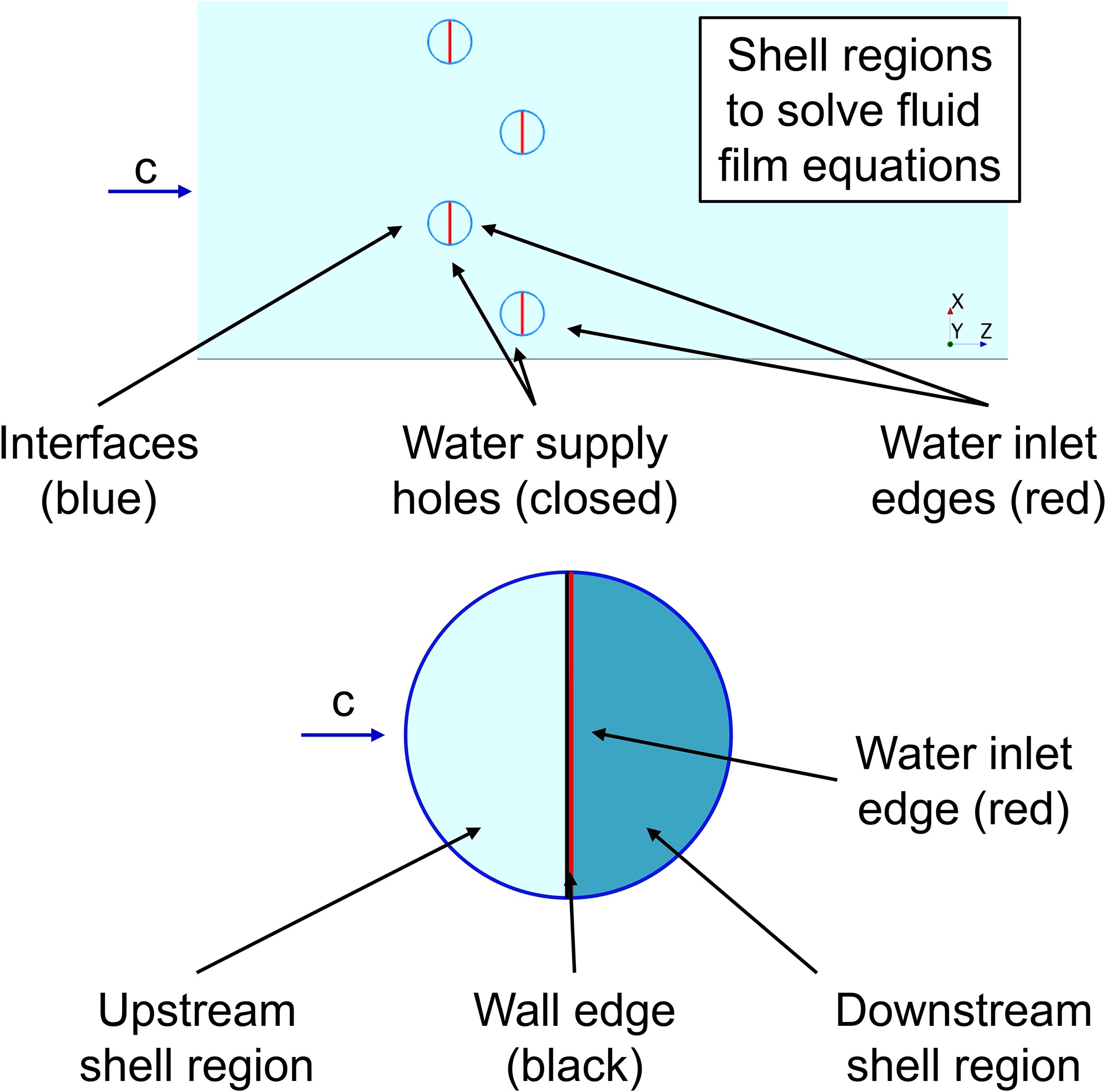
This setup represents a significant simplification in terms of water injection, but is considered acceptable due to the relatively large distance to the extraction slot.

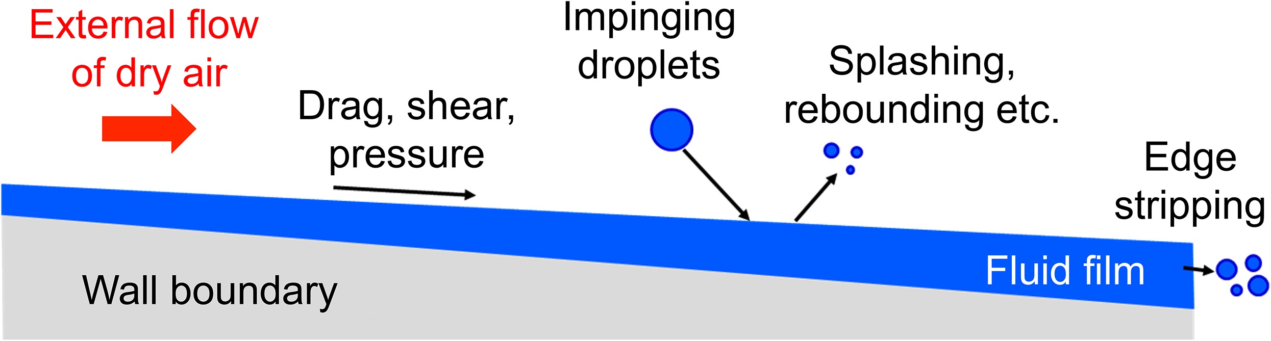
At the interface between the fluid film and the air continuum, a multiphase interaction model is established. The main interaction phenomena are illustrated in Figure 5. Among gravitational effects, the main drivers of the fluid film flow are shear forces and pressure gradients induced by the surrounding air flow. The film height is a direct result of the film’s flow rate and induced flow velocity. Evaporation and/or condensation are not considered in the investigation due to the comparatively low ambient temperature.

Figure 5.

Interaction phenomena of the different fluid phases.

The application of the edge stripping model models the ejection of droplets from the film flowing over a sharp edge. The criterion for edge stripping is based on the force balance between the fluid film’s inertia, surface tension and gravity and formulated as force ratio FR (see Equation 1).

Wef is the fluid film weber number, Bof is the Bond number, Lb is the break-up length and hf the fluid film thickness. The model is applied at edges whose angle θ exceeds a threshold value which is set to 10deg in this study. Edge stripping occurs when the force ratio exceeds a user-defined critical force ratio whose default value is 1 (please refer to the STAR-CCM+ User guide).

In turn, droplets which are impinging on a wall associated to the shell region contribute to the formation of a fluid film. The Bai-Gosman model is applied to account for the different modes of wall impingement (cf. Figure 6) in dependency of the incident Weber-Number Weinc which is defined in Equation 2.

Figure 6.

Wall impingement modes according to the Bai-Gosman model.

The Weber-Number describes the ratio of the inertia of a moving droplet to its surface tension and is defined by the droplet’s parameters density ρd, diameter dd, surface tension σd and velocity normal to the surface cd,n. Within the study presented within this paper only adhere, rebound and spread are considered as possible modes of impingement. For the unsteady simulation runs, a time step of 5.0E-5s (35 inner iterations per time step) is considered to accurately capture physical phenomena and to ensure a stable simulation run in light of the huge impact of mass, momentum and energy transfer in case of wall impingement and the transition to film. Every simulation has been run until the characteristic quantities such as collection rate is converged to a near steady-state value.

The 3D-URANS equations of the air phase are closed by application of the SST k-ω turbulence model (two-equation model). The gravity is considered in the simulations. Air and liquid water are both considered with temperature dependent dynamic viscosity, specific heat and thermal conductivity (REFPROP data). Air is modelled as ideal gas in this analysis. As the REFPROP data for surface tension is based on the assumption of a planar interface between liquid and gaseous phase, the calculated surface tension values are multiplied by a factor of 0.85 in case of the spherical liquid particles as suggested by Li et al. (2010). Volume source smoothing and shell source smoothing are activated for the two-way coupling of continuous air phase and liquid particulate phase within the Lagrangian Multiphase solver. Both smoothing methods promise an improved numerical stability without altering the solution, particularly in case of Lagrangian parcels entering a fluid phase volume or in case of impingement on a fluid film in a shell region.

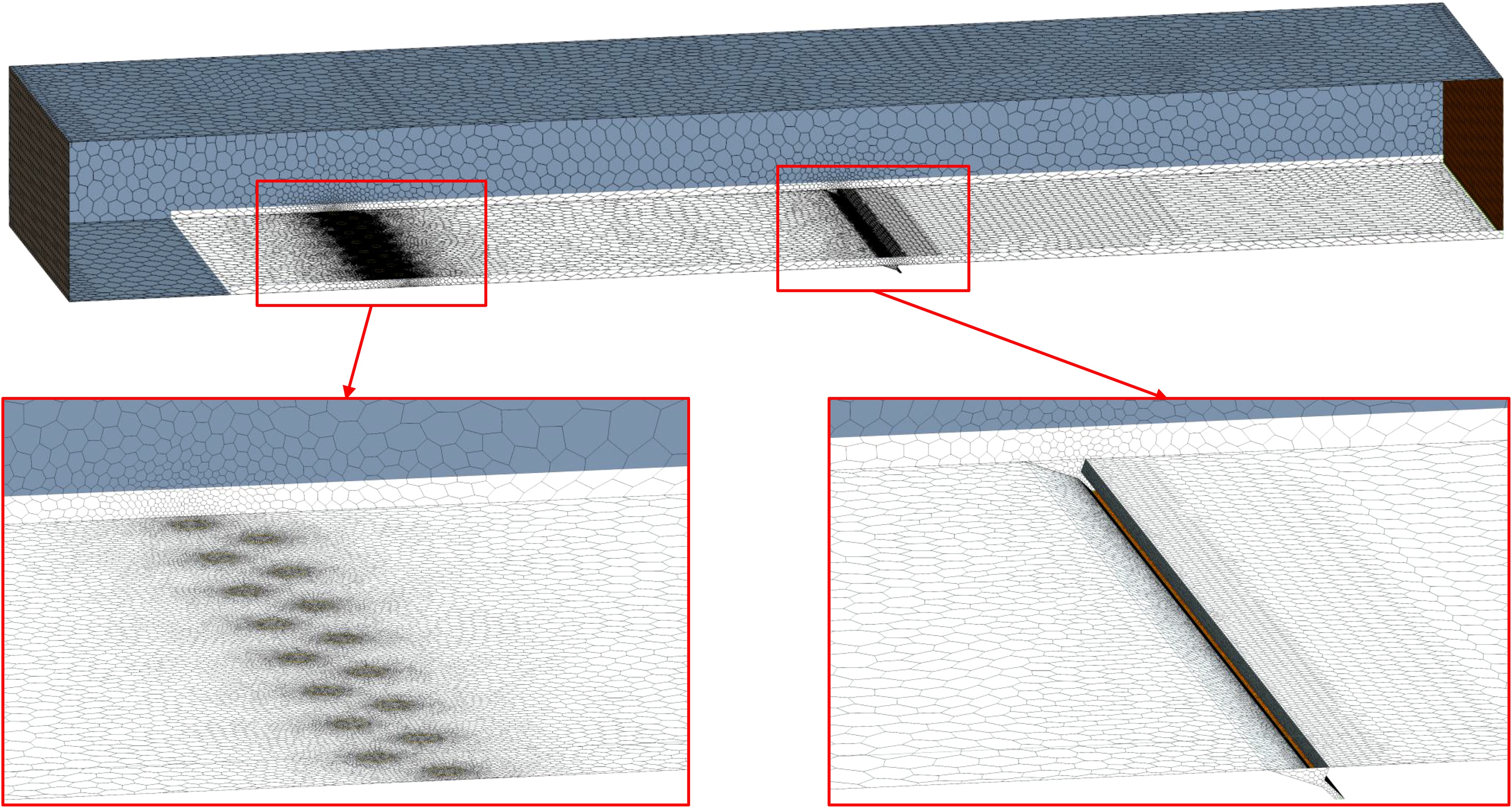
The mesh generation is carried out directly in the CFD solver STAR-CCM+ and contains unstructured polyhedral cells with local refinements in the vicinity of the flat plate surface, the suction slot and the water supply holes to adequately resolve the circumferential curvature. Furthermore, inlet and outlet surfaces are refined. No prism layers are applied to resolve the boundary layer flow. These settings in combination with a cell base size of 10 mm lead to a total number of 258,663 cells for the simplified geometry of the flat plate test rig. The fluid film shell regions contain 40,527 cells overall. Figure 7 gives an impression of the mesh.

Figure 7.

Computational mesh considered in the CFD simulations.

Results and analysis

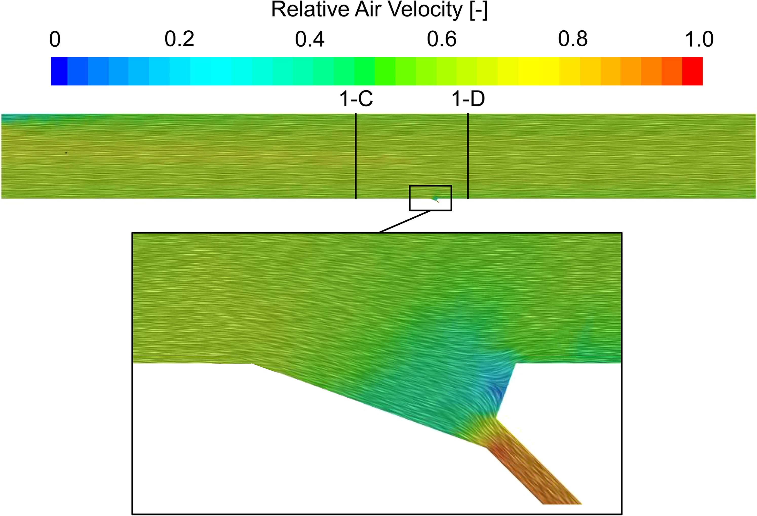
The fluid film’s velocity and thickness is mainly driven by the shear forces of the surrounding air flow. In Figure 8 the flow field is visualized on lateral section 1 (cf. Figure 3). The air-flow is dominated by an axial flow direction while only in the vicinity of the slot the flow exhibits a downward vertical component with an acceleration of the flow due to the reduction of the cross-sectional area at the exit of the extraction slot. Furthermore, a stagnation point can be observed at the downstream edge of the slot. Despite the difference between individual cases in terms of air flow velocity and water supply mass flow rate, a large qualitative agreement (of flow features etc.) is found between them. Thus, in the following paragraph the results are discussed only for one case and subsequently a comparative analysis of all cases is provided.

Figure 8.

Distribution of velocity magnitude on lateral section 1 (case 1) extracted from CFD.

Distributions of velocity magnitude in wall-normal direction are depicted in Figure 9. Within the plots experimental data is compared with numerical results, both extracted at positions upstream and downstream of the extraction slot, respectively.

Figure 9.

Distribution of velocity magnitude normal to the flat plate surface (case 1).

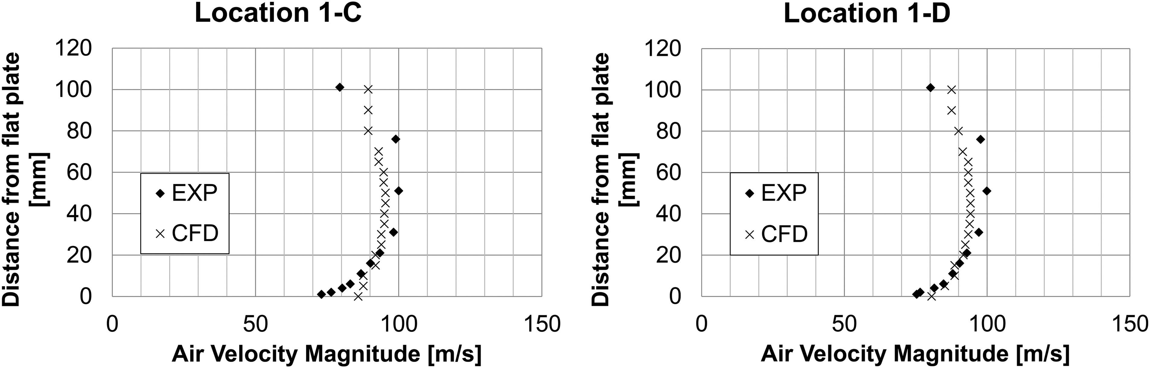
From the comparison, it can be concluded that the order of magnitude of the predicted air velocity is in good agreement with the measured data. However, slight deviations are found in the in proximity of the flat plate. One reason for this might be the mesh resolution close to the wall as no prism layers are applied to resolve the boundary layer flow as a compromise between accuracy and calculation speed. Another reason might be the simplification of the injection holes. In the experiment, the injection holes are open and in the simulations they are closed. The interaction between the airflow and the injection holes could be visible in the deviation of the results.

In Figure 10 the time-instantaneous distribution of the relative fluid film thickness of case 1 is visualized in a top view.

Figure 10.

Time instantaneous distribution of fluid film thickness on the flat plate (case 1) extracted from CFD.

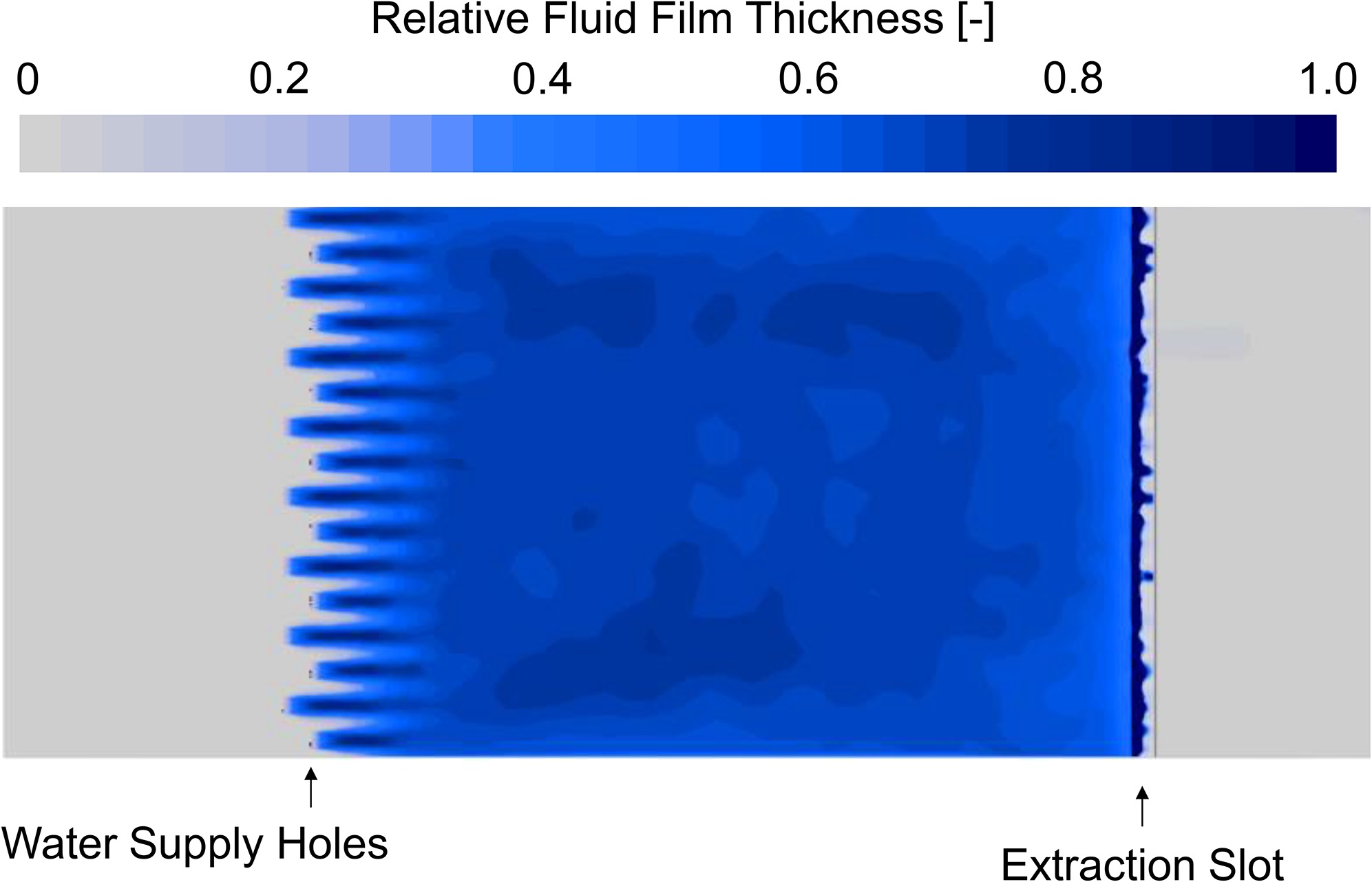
It can be observed that the injected water enters the shell-domain in fan-shaped jets which merge downstream of the water injection bores into a relatively homogenous fluid film and covers the complete width of the flat plate and continues to flow in the direction of the slot. While the single injection-jets exhibit locally increased film thicknesses due to the carried mass, the film thickness equalizes downstream of the merging position.

In Figures 11 and 12 the distribution of both the fluid film thickness and the fluid film velocity extracted from one lateral section are plotted in stream-wise direction for the considered cases.

Figure 11.

Comparison of fluid film thickness on lateral section 1 for all cases extracted from CFD.

Figure 12.

Comparison of fluid film velocity on lateral section 1 for all cases extracted from CFD.

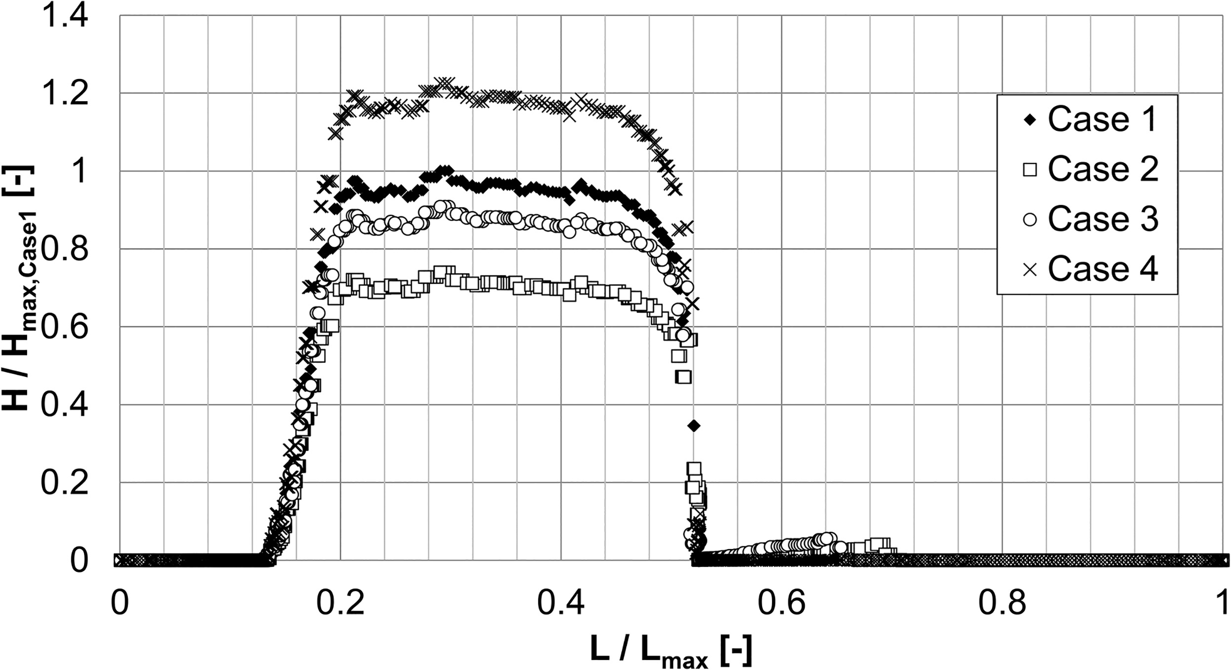
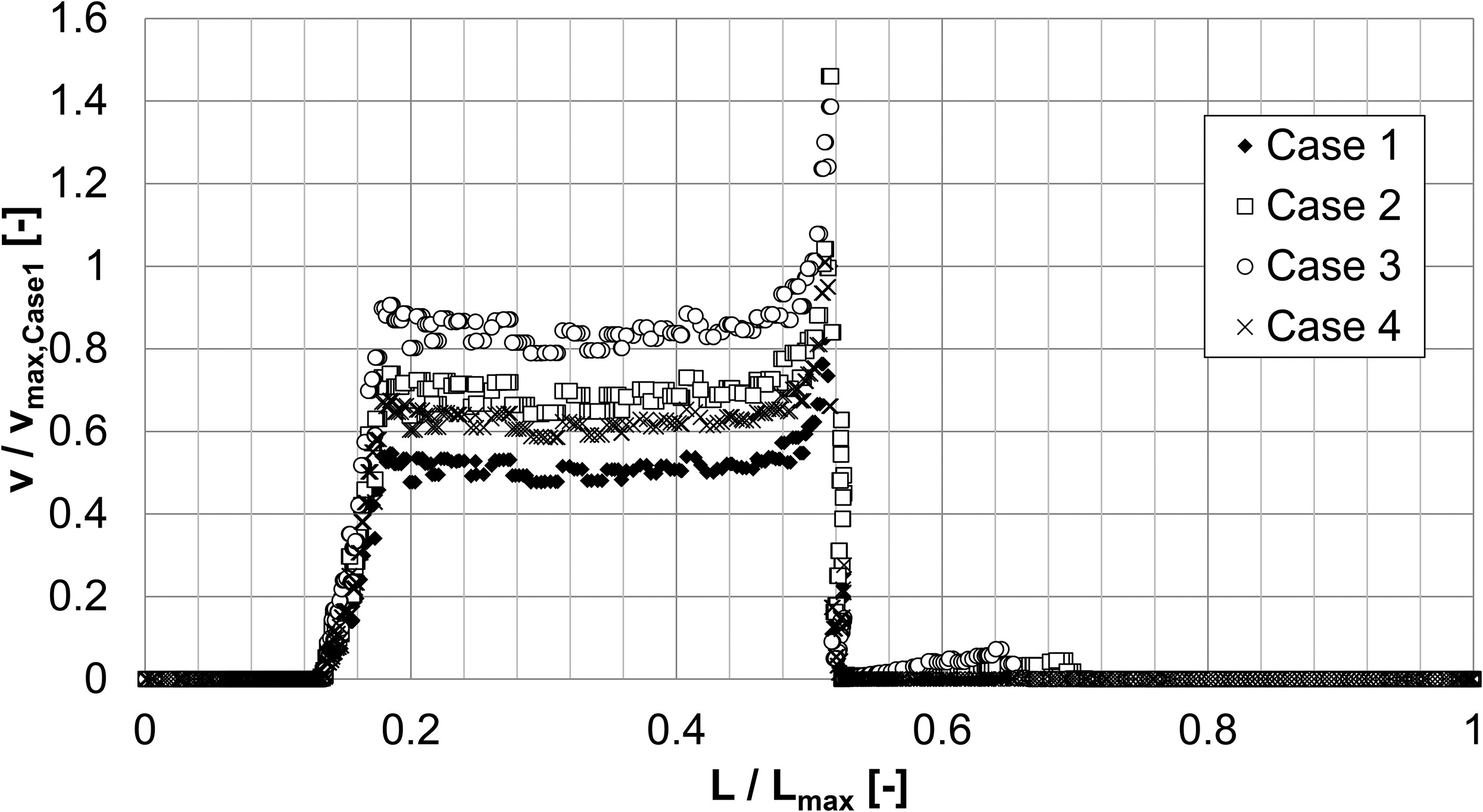
Qualitatively, all distributions have the same shape and show the same characteristics. After a continuous increase of film thickness and velocity in the vicinity of the injection jets the film shows almost constant properties and covers most of the flat plate surface. Ultimately upstream of the extraction slot at L/L_max = 0.52, the fluid film thickness is decreased and the velocity is increased locally as a result of additional acceleration by air and gravity.

Due to the increased air velocity and therefore increased shear forces acting on the fluid film, the fluid film velocity is increased globally for case 2 in comparison to case 1 while the fluid film thickness is decreased at the same time. An enlarged water flow rate (case 3) with constant air velocity yields a rise in fluid film thickness with simultaneous increase of fluid film velocity. The larger water flow rate of case 4 in comparison to case 1 confirms the trends as found before.

After discussing the characteristics of the fluid film velocity and thickness on the main portion of the flat plate, in the following the fluid film behavior within the slot geometry shall be described in more detail. The vicinity of the slot is shown magnified on the left side of Figure 13 while on the right side a photograph is shown which corresponds to the experiment performed with identical operating conditions.

Figure 13.

Comparison of numerical and experimental fluid film distribution in the vicinity of the extraction slot (case 1) (left: CFD, right: experiment).

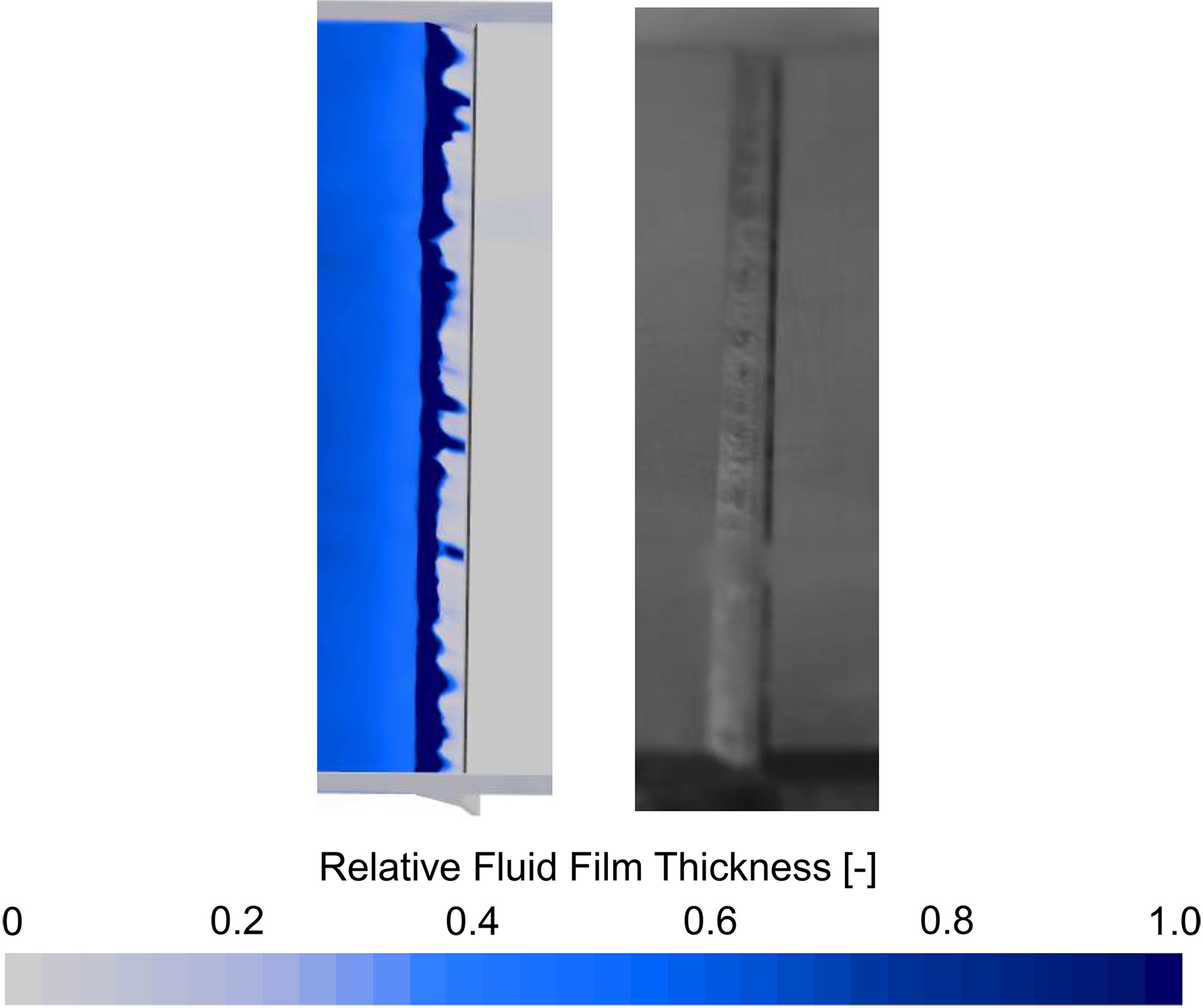
Once the fluid film has travelled the distance between the injection holes and the extraction slot, it enters the inclined surface of the slot in individual rivulets instead of a homogenous film. Those rivulets are also present in the experiments as can be seen in Figures 1 or 13 which indicates the qualitatively correct reproduction of this phenomenon. The formation of those finger-like structures at the advancing front of the spreading film is mainly influenced by the ratio of gravity and surface tension (Slade, 2013). The figure also shows that a non-negligible amount of water flows past the slot via the side-walls.

After flowing past the edge to the first inclined surface of the slot, the fluid film accumulates to regions of increased thickness. After a critical thickness and thus momentum flux is reached, those rivulets start to flow.

Instead of flowing over the edge, the fluid film can also be converted into droplets via the effect of edge stripping. As discussed above, the driving force for the edge stripping is the ratio between the film momentum flux to the surface tension and gravity. Thus, the local fluid film thickness as well as fluid film velocity at the edge is the key driver of the edge stripping effect. As soon as droplets are shed from the film, the film thickness is reduced as the mass of the individual stream is depleted which ultimately leads to the reduction of stripping intensity.

Generally, the sequence of build-up of fluid film thickness and velocity at the edge, stripping of particles and depletion of mass yielding decreased film thicknesses is a periodic process and can be observed constantly within the slot geometry. Figure 14 illustrates the sequence of this process with a series of instantaneous snapshots. The shown sequence corresponds to a physical solution time of 2.5 ms.

Figure 14.

Temporal sequence of fluid film build-up and edge stripping within the extraction slot extracted from CFD.

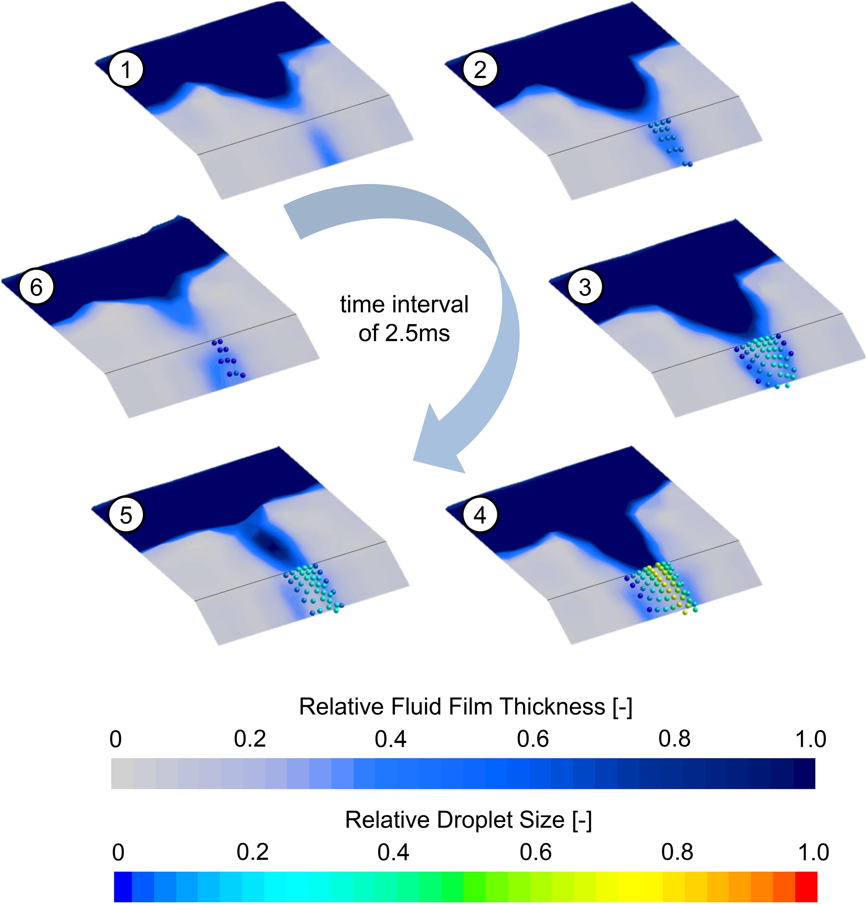
The particles which are shed from the film are accelerated by the moving air and are mostly carried by the air flow and leave the simulation domain. Depending on their trajectories, some particles impinge on the downstream surface of the slot, accumulate and eventually transition into fluid film before leaving the domain.

Due to the dependency of the edge stripping intensity on the fluid film’s properties (thickness and velocity) and the surrounding air velocity, the second edge of the extraction slot’s geometry is more prone to shedding of droplets than the first edge as the air velocity and film thickness are locally increased (cf. Figures 8 and 13). However, edge stripping at the upstream edge is still present and droplets shed from the film at this position and can contribute to the development of fluid film downstream of the slot. This mechanism is visualized in Figure 15.

Figure 15.

Mechanism of fluid film development downstream of the extraction slot (schematic).

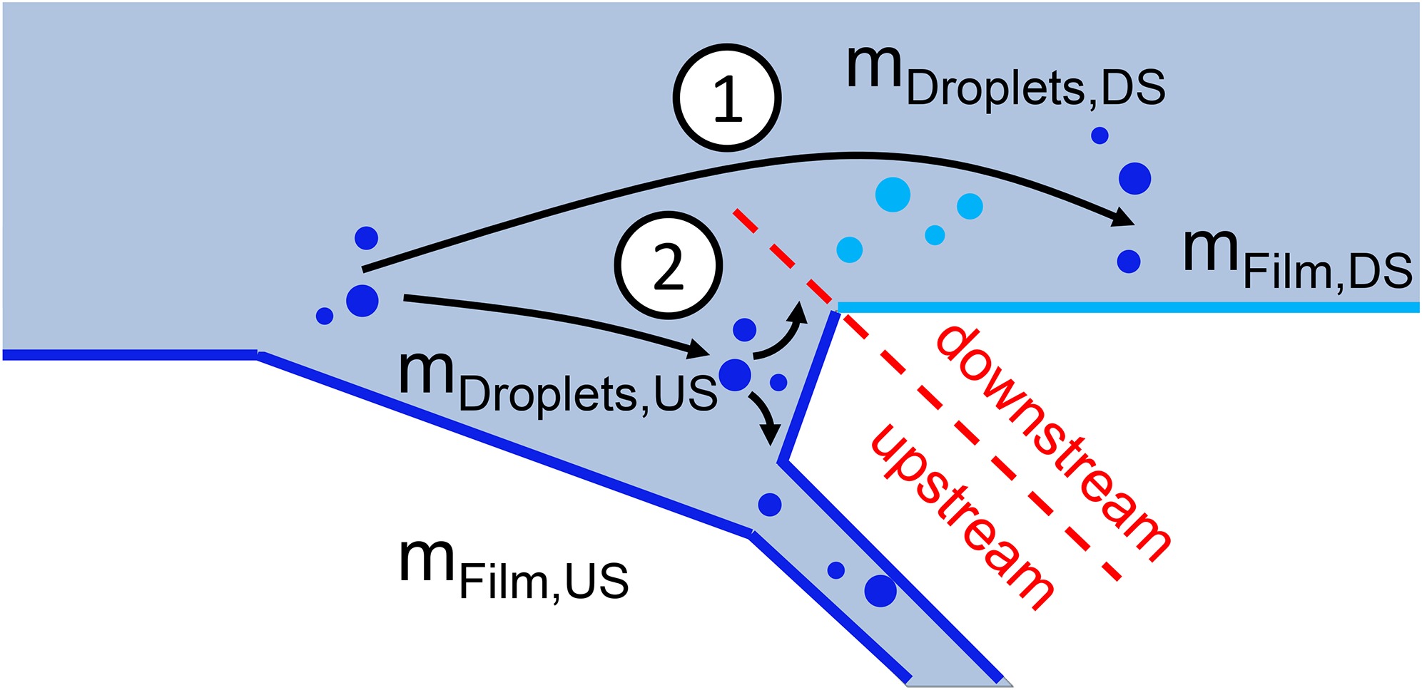
There are three transport mechanisms to carry liquid water downstream of the slot. First, droplets whose momentum is sufficiently large for them to fly past the slot impinge on the flat plate surface and transition into fluid film (denoted with 1 in the figure). Second, droplets which impinge at the blunt edge and transition into film (denoted with 2 in the figure). The resulting film is then driven in both positive and negative vertical direction due to the stagnation point flow at the blunt edge (cf. Figure 8). The upwards moving film either flows in stream wise direction (depending on the film momentum flux) or sheds droplets in another edge stripping event which are transported by the air. Third, film which flows past the extraction slot at the side walls of the domain (not shown in the sketch) which can also be spotted in Figure 13. This is in qualitative agreement with the provided data.

From the water masses found upstream and downstream the extraction slot, a collection rate CR can be computed (Equation 3) which is one of the main performance values used in this paper.

All water mass which leaves the domain via the slot as well as the water which is present in the form of droplets or film upstream of the highlighted position in Figure 15 is accounted to the collected water mass m_collected. However, all mass which exits the domain through the main outlet as well as the water which is found as droplets or film downstream of the slot is accounted to uncollected water m_uncollected.

The extraction slots do not only remove water in the form of film and droplets but also working fluid which in case of a steam turbine leads to a reduction of the steam mass flow participating in the expansion and thus a degradation in power output and overall efficiency. Thus the air leakage is another performance value for the assessment of extraction slot geometries or operation conditions. The collection rate is compared with experimental data for the four investigated cases in Figure 16. The data below is given as ratio to the results of case 1 (denoted with ref).

Figure 16.

Comparison of collection rate from CFD with experimental data.

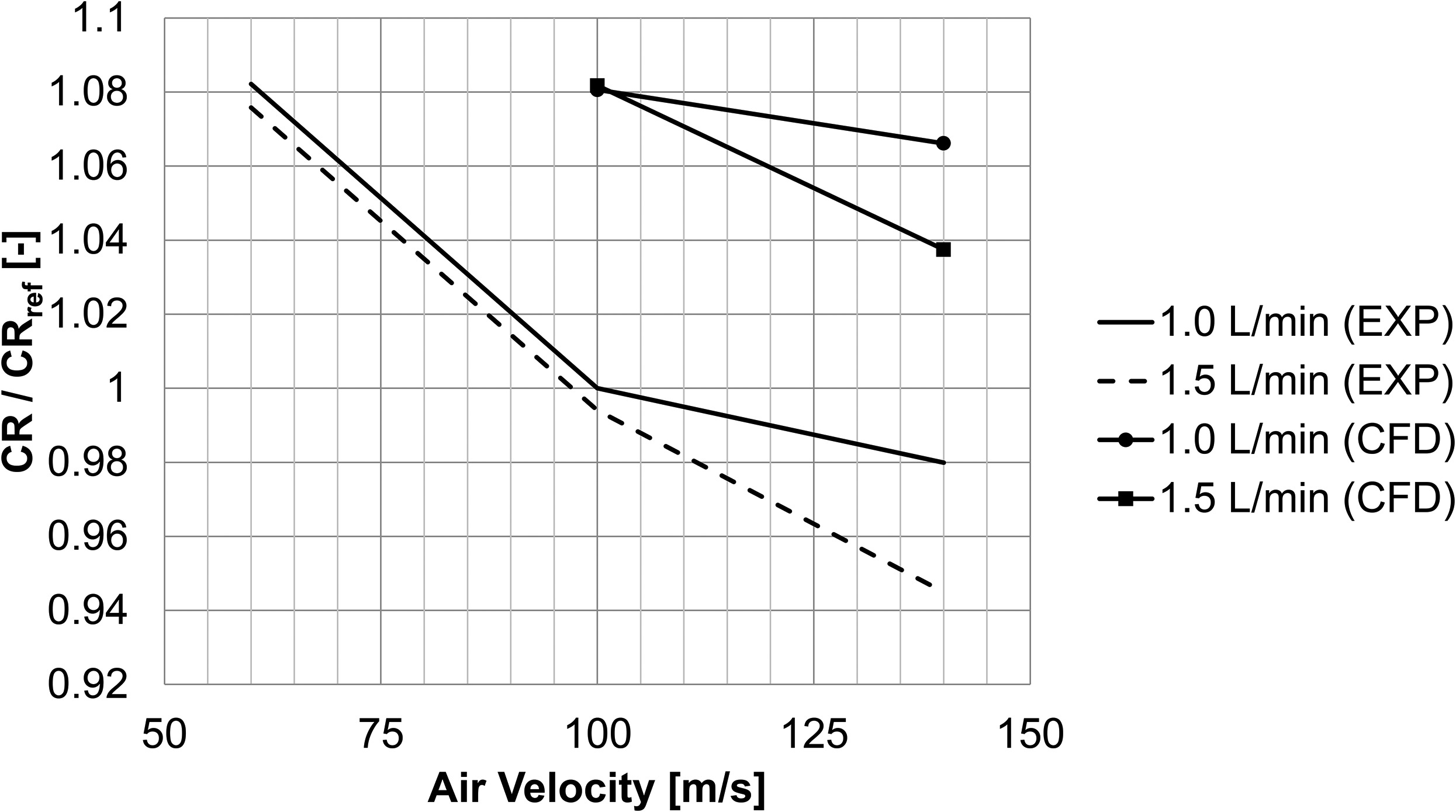
In general, the collection rates predicted by the CFD analysis are larger than measured in the experimental tests. However, when analysing the change of water collection rate in dependence on the two influencing factors air velocity and water mass flow rate qualitatively, one can find that the predicted results are in good agreement with the experimental data. The increase of air velocity from 100 m/s to 140 m/s leads to a drop in collection rate of 1.3%-points for 1.0 L/min water flow rate as estimated by the CFD while the experiments revealed a drop of 2%-points. A further increase of water mass to 1.5 L/min flow rate entails another drop of 2.7%-points in the numerical prediction while the experiments showed a decrease of 3.5%-points.

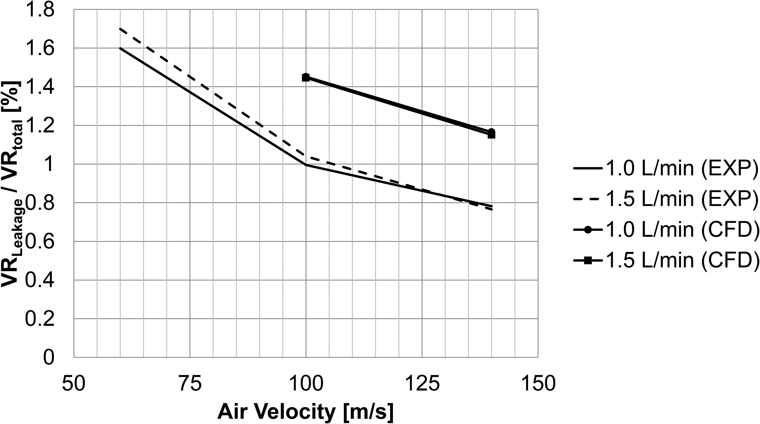
The ratio of air leakage to the individual total volume flow rate per case is plotted in dependency of the water mass flow rate and air velocity in Figure 17. As discussed for the collection rate, also the air leakage is increased in comparison with the experimental results. However, the qualitative dependency on the influencing factors can be shown.

Figure 17.

Comparison of air leakage from CFD with experimental data.

Figures 18 and 19 draw a comparison between the predicted results and the provided data in terms of fluid film thickness and fluid film velocity. Again, the values are given as ratio to the result of the chosen reference case (case 1).

Figure 18.

Comparison of fluid film thickness from CFD with experimental data (position C).

Figure 19.

Comparison of average fluid film velocity from CFD with experimental data (position C).

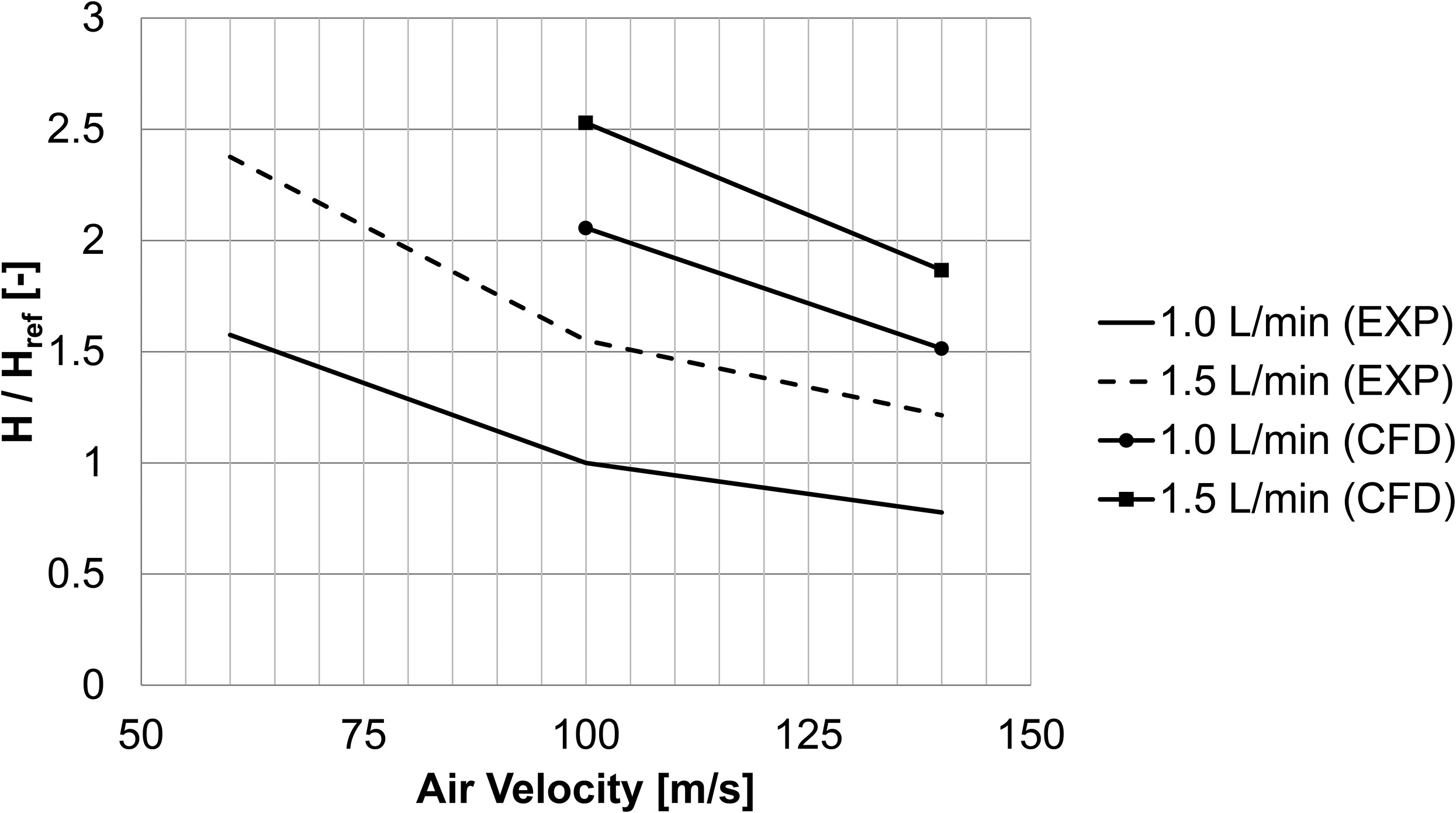
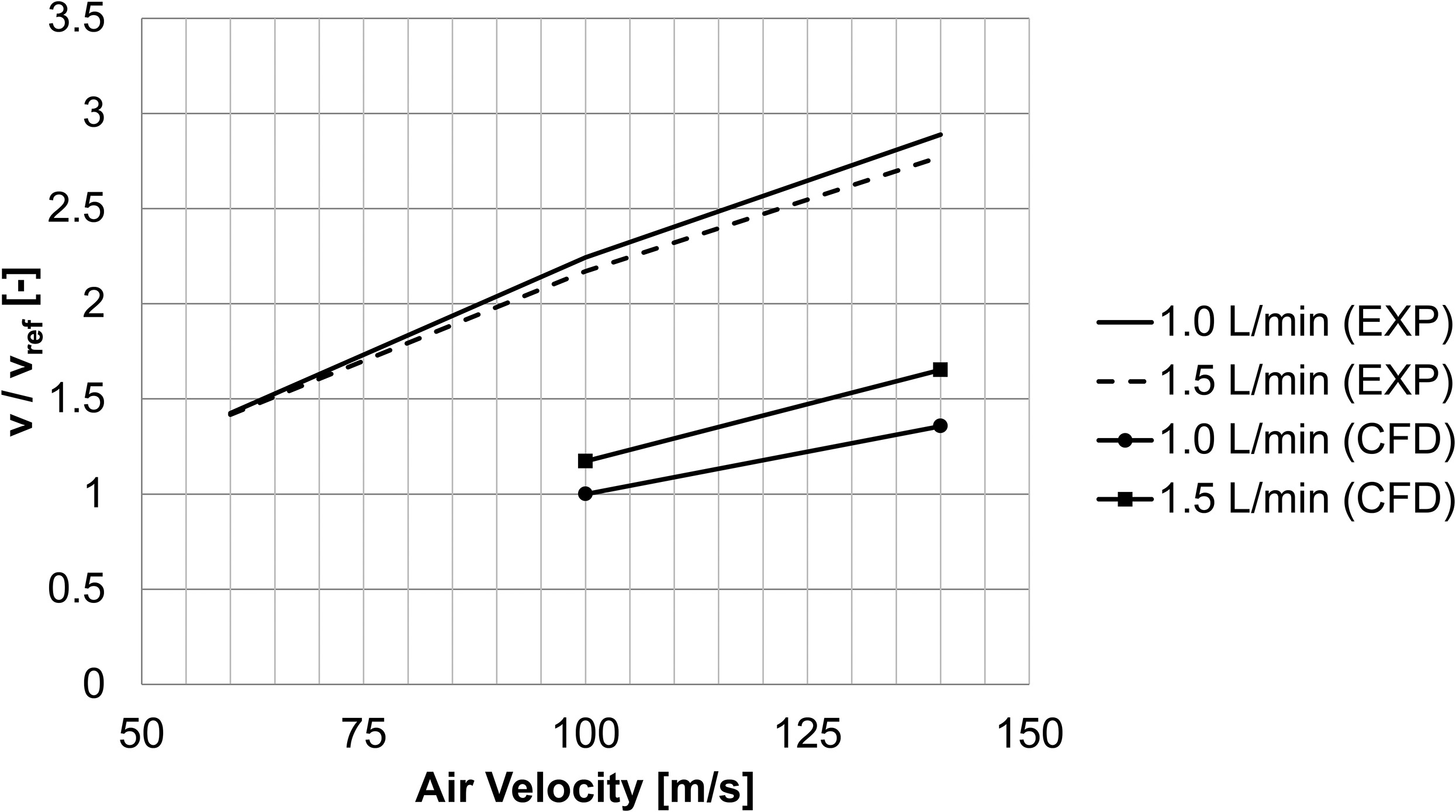
It can be seen, that the predicted film thicknesses are generally larger than the measured values whereas for the velocity the situation is reversed. This in combination with the over predicted air velocities might be an indication for an underestimation of the drag force acting on the fluid film.

However, another point needs to be taken into account in this analysis. The overestimated collection rates could also be explained by the limits of the computational model. As explained above, the side wall allows for film formation only on a relatively small vertical portion of the complete wall (5 mm of height) and therefore the amount of water which is able to flow past the slot is limited. Since in the experiments the complete side walls allow for film formation, the potential for water transport is increased and thus the measured collection rates might be distorted.

Finally, when comparing the qualitative change between the individual cases, the general influence of increasing the air velocity and water flow rate is predicted well by the CFD simulations.

Conclusion

In conclusion, the comparison of the four cases with the experimental data demonstrates that the chosen simulation approach is able to predict the main features and characteristics of film flow and interaction with the surrounding air and is therefore able to be applied in the optimization of slot geometry and the position on the airfoil. The collection rates as well as fluid film properties show the same qualitative dependency from the water flow rate and the air velocity. Still, an offset is being found in comparison to the measured data which identifies improvement potential of the simulation setup in terms of mesh settings or tuning of the parameters applied by the models such as the intensity of the drag force (drag coefficient) or the surface tension. Further measurements (e.g. within the slot, etc.) can also help to investigate the present deviations and further improve the prediction quality of the simulations.

Nomenclature