
Introduction
In by far the biggest area of a turbine map both the stator exit Mach number and the rotor exit Mach number (in the relative system) are high. In this map region the similarity laws for incompressible flow are of little value for extrapolation purposes. However, for extending a turbine map to the low mass flow region - where turbines operate in a windmilling engine - correlations derived from incompressible flow theory are very helpful.
Theory
Work and flow coefficient
If we consider the form of the ψ-Φ relationship for a single stage turbine with symmetrical velocity triangles in simple terms, we can conclude that the work coefficient ψ is a linear function of the flow coefficient Φ. This follows from the fact that the flow leaves a blade or vane row in the direction given by the trailing edge geometry (see Figure 1).
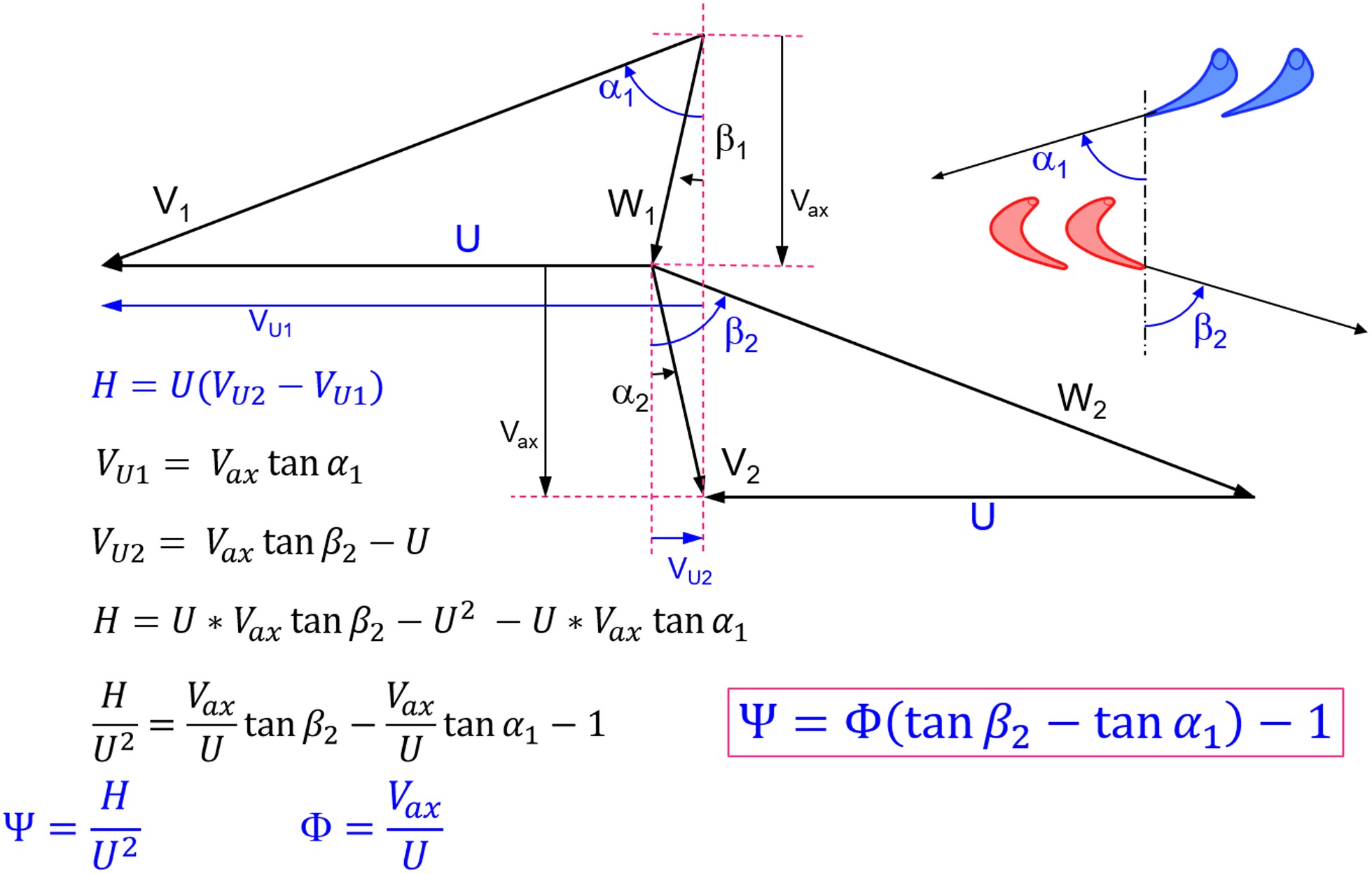
The work output H is a straight line when plotted as Ψ over Φ, whereas work input His – calculated from pressure ratio - is not (see Figure 2).
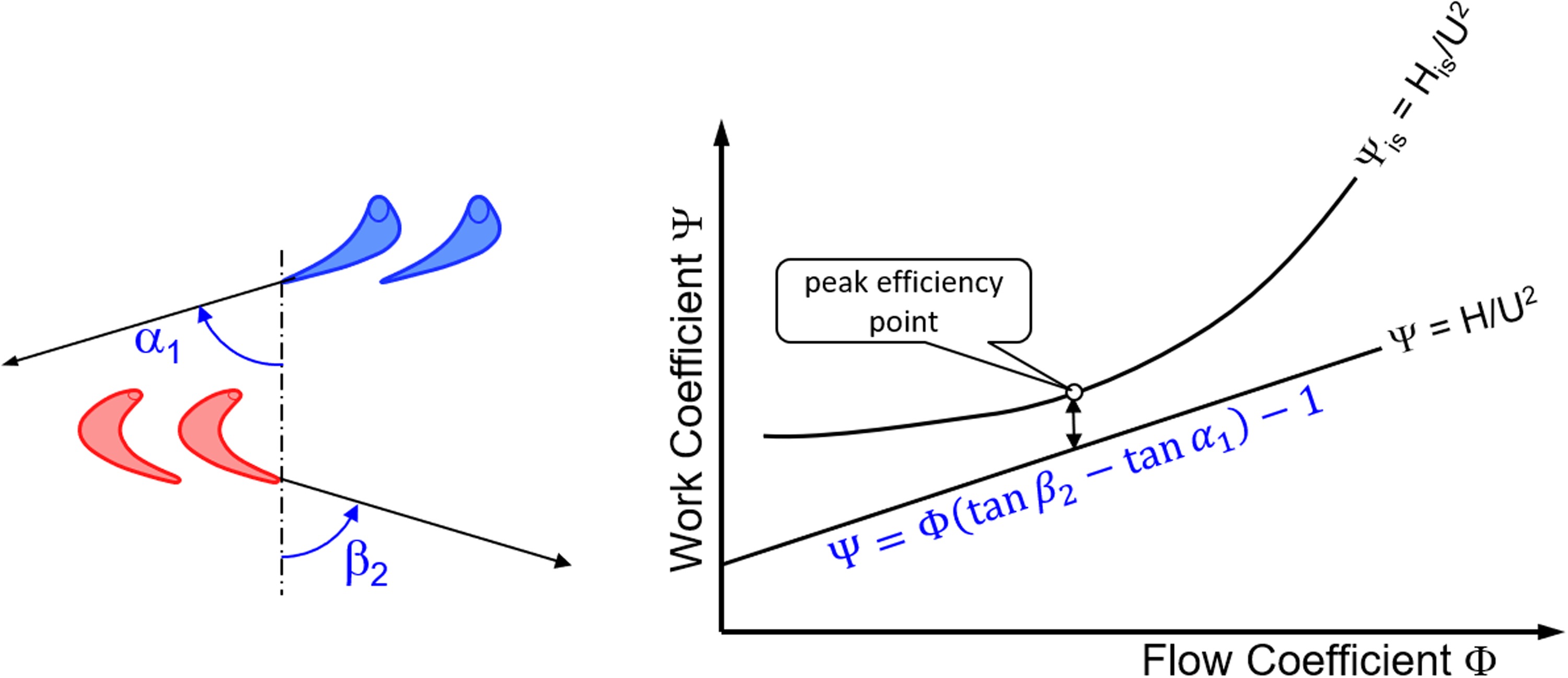
The losses in the expansion process, described by efficiency η = H/His, are smallest at the peak efficiency point.
The only prerequisite for the validity of Equation 1 is that the (relative) flow direction downstream of the blades and vanes is enforced by the geometry of the blades and vanes. Furthermore, in an incompressible fluid (constant density), there is only one curve for ψis = f(Φ) and this is valid for any speed.
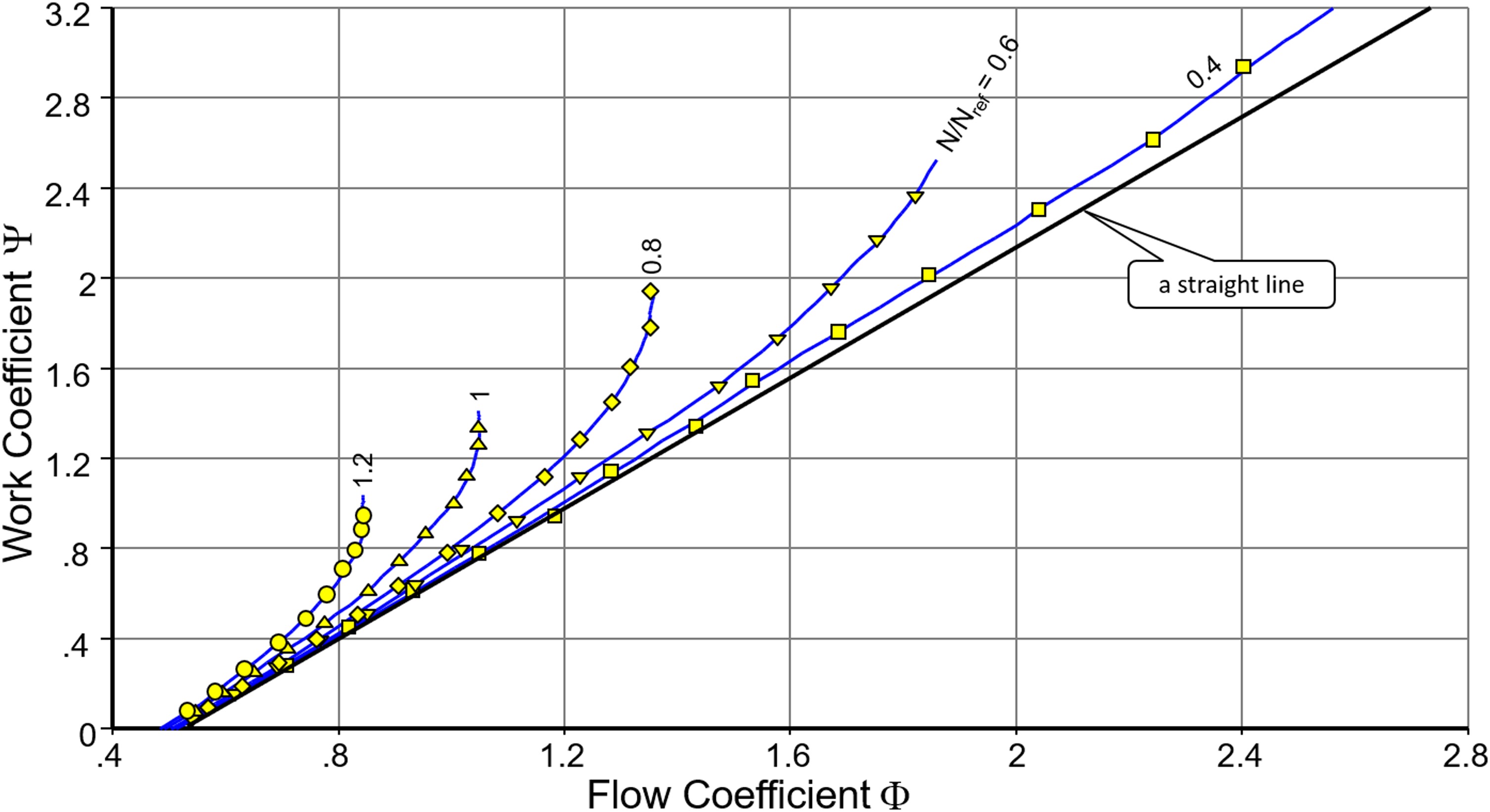
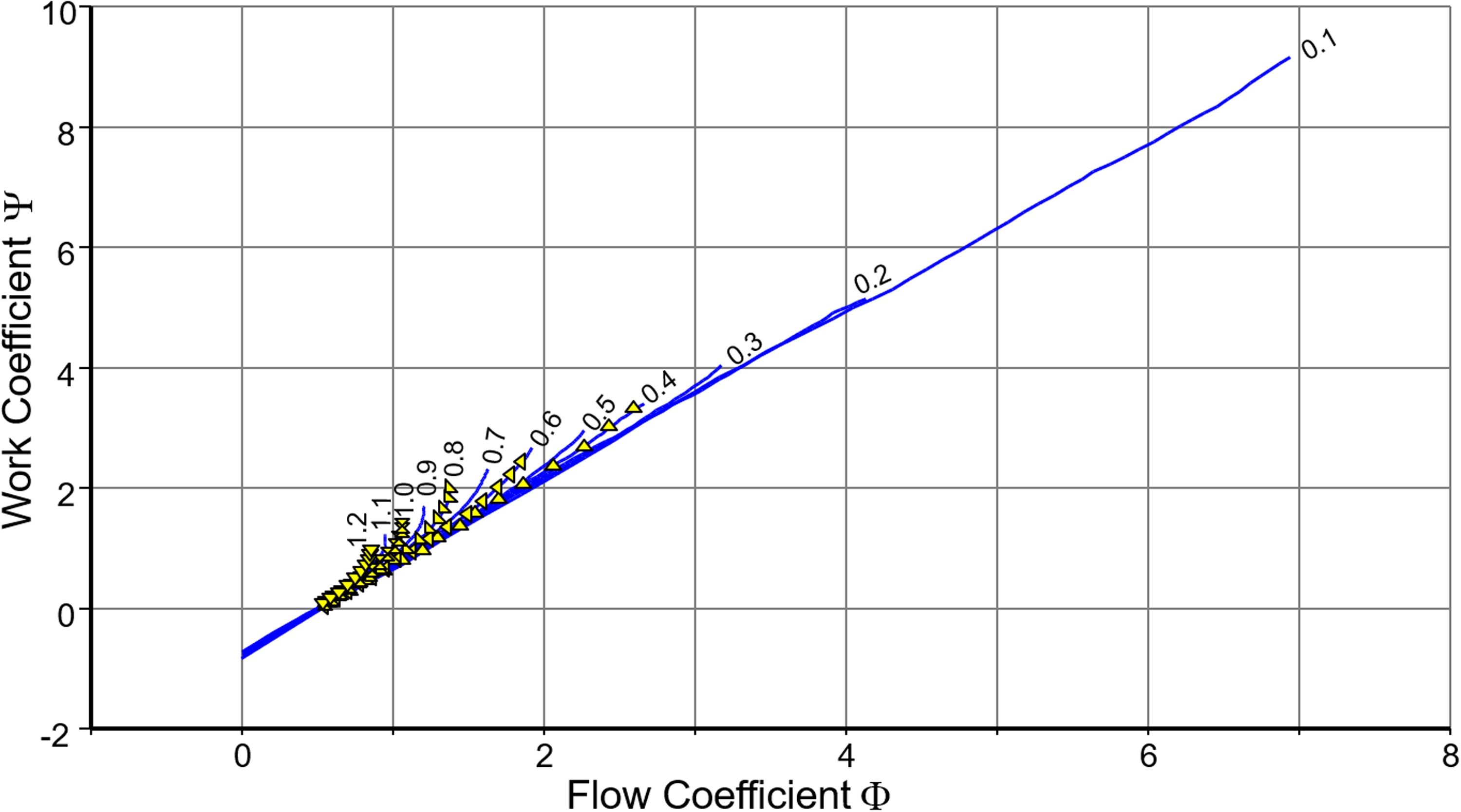
Figure 3 shows data published by Broichhausen (1994) with lines for Ψ plotted against flow coefficient Φ. The lower the speed, the more the Ψ-Φ correlation is a straight line.
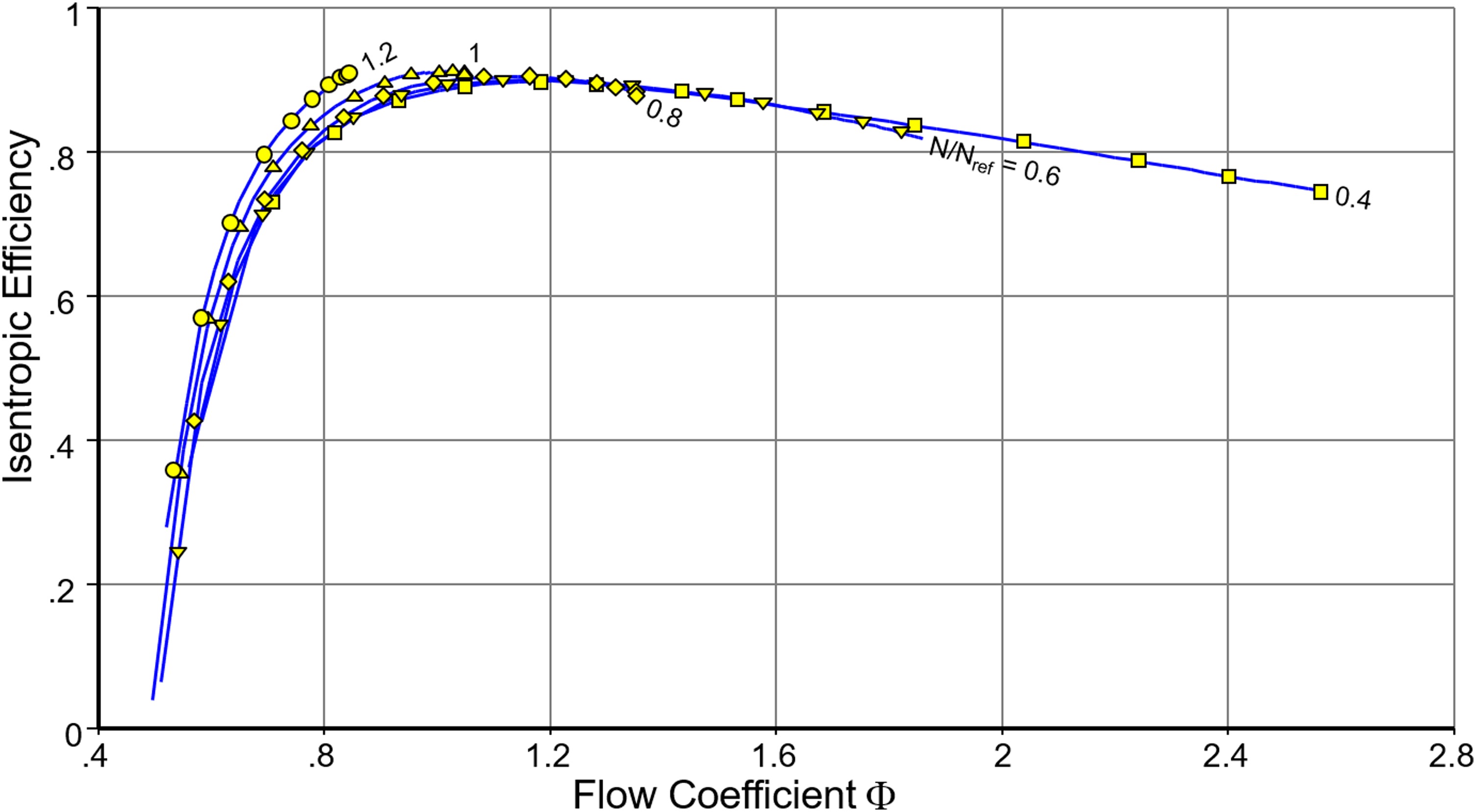
Efficiency
Figure 4 shows the efficiency values corresponding to Figure 3. For the relative speed values 0.4, 0.6 and 0.8 the efficiency lines collapse in the region where flow coefficients are less than Φ ≈ 1.2, where the peak efficiency values occur.
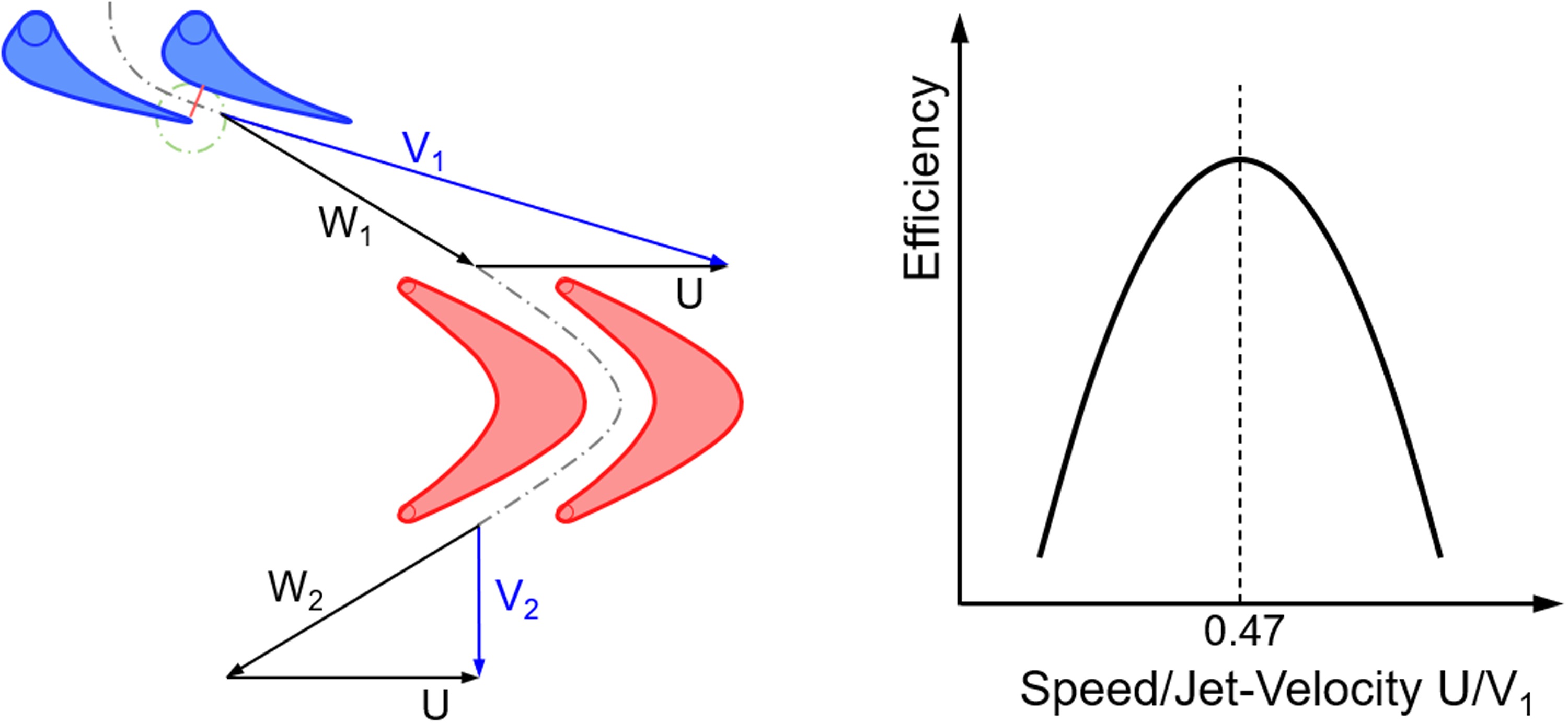
Another efficiency correlation originates from theoretical considerations about impulse turbines. In such a turbine the inlet guide vane works like a nozzle which produces the jet velocity V1. There is no velocity change in the rotor of an impulse turbine (W2 = W1) as can be seen in Figure 5. Maximum efficiency is achieved when the direction of the absolute velocity V2 at the turbine exit is axial. The ratio of U/V1 for optimum efficiency is approximately 0.47.
Experience from working with the maps of many single- and multi-stage turbines has shown that efficiency generally correlates well with the speed/jet-velocity ratio. Figure 6 demonstrates this for the same turbine as used for Figure 3.
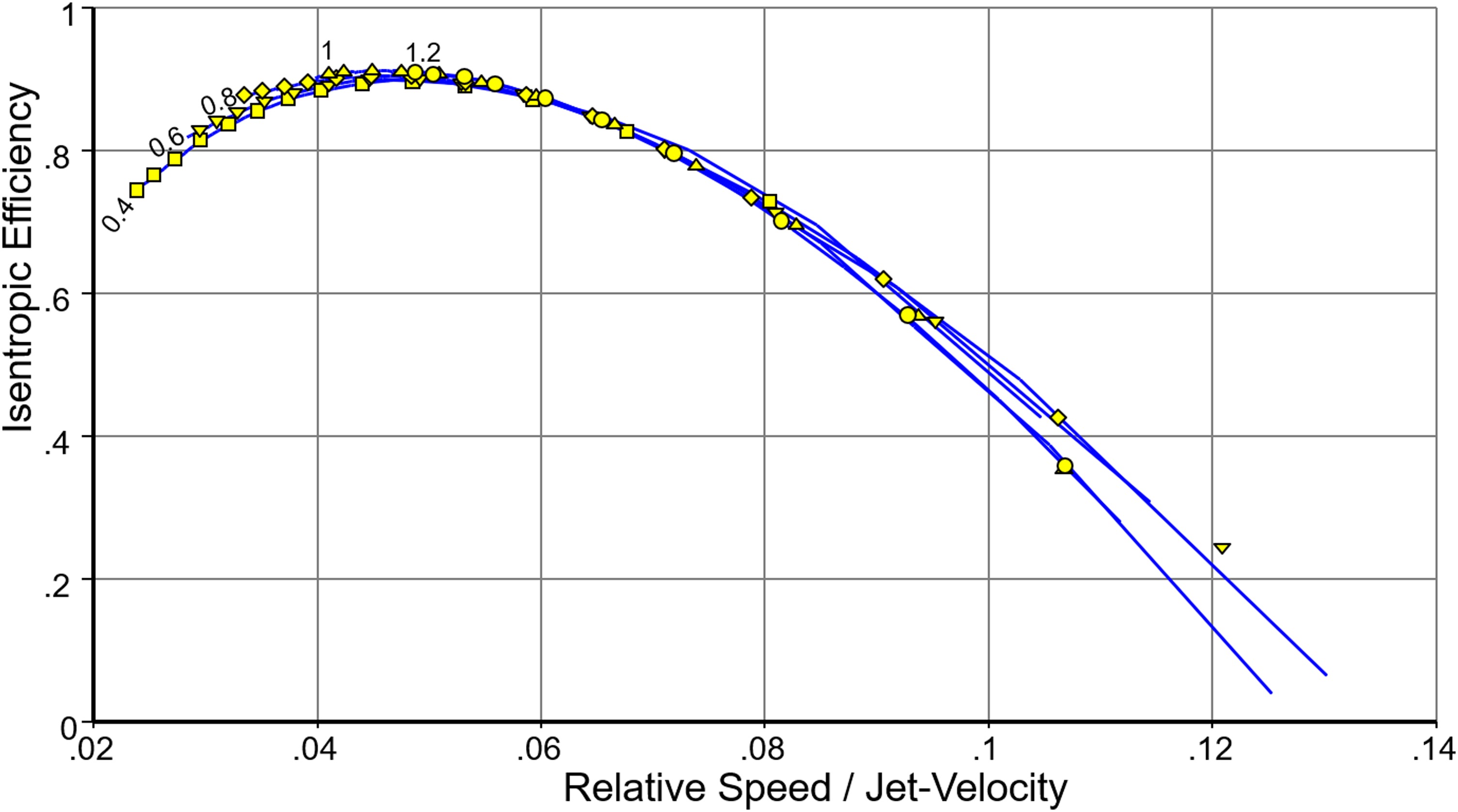
Note that Figure 6 does not employ the absolute circumferential speed U – it uses relative speed N/Nref. The x-axis numbers in Figure 6 therefore differ in magnitude from the value shown in Figure 5.
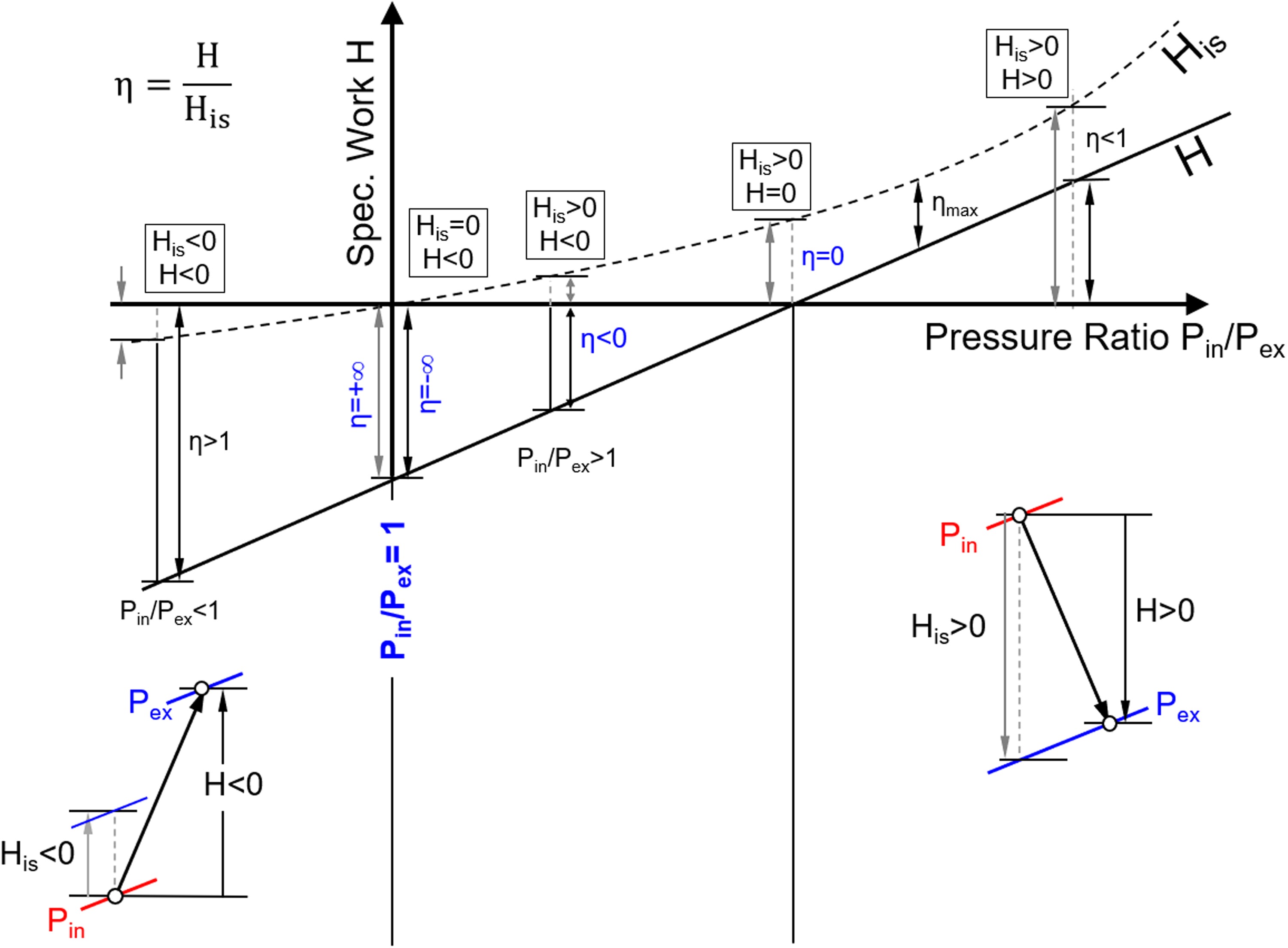
The correlations of efficiency with flow coefficient and speed ratio are useful only in the region with positive effective work Heff. Efficiency is zero if effective work is zero and drops to minus infinity when pressure ratio is 1, see Figure 7.
Torque
Turbine power can be expressed as the product of flow and specific work as well as the product of angular speed and torque:
Rearrangement and insertion of Equation 1 yields
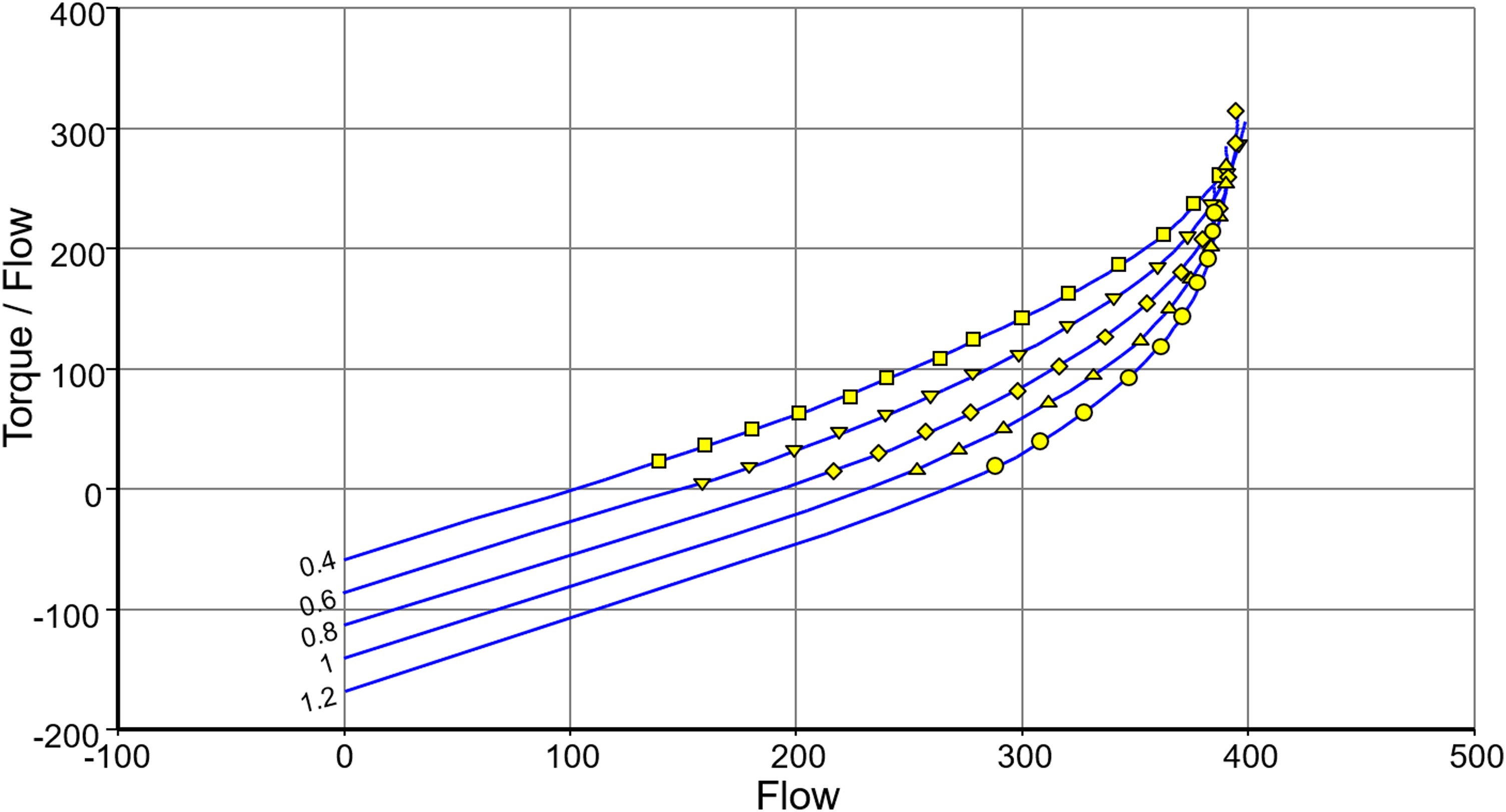
This equation is valid where flow velocity Vax is proportional to mass flow m, in the incompressible flow region. Under this condition, Trq/m² is a linear function of 1/Φ and Trq/m is – for a given circumferential speed U – a linear function of m:
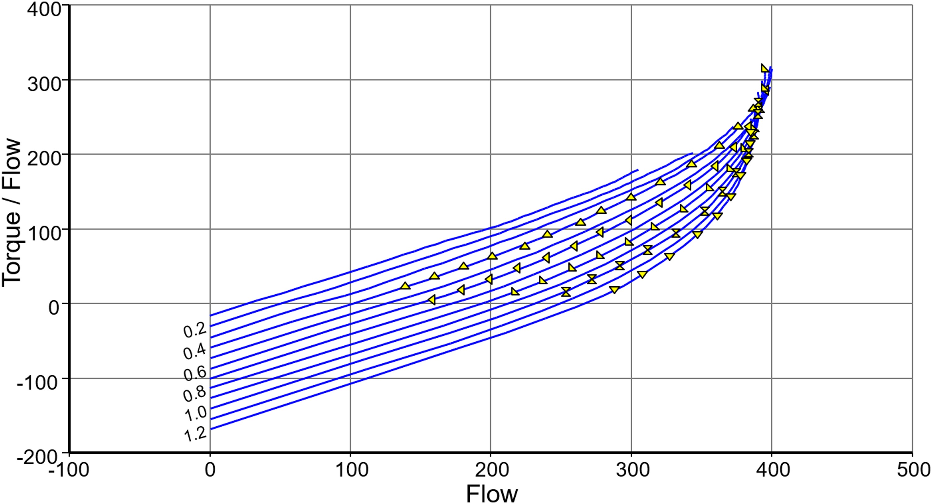
Figure 8 shows that Equation 4 is in line with measured data in the low mass flow parts of the speed lines. The dashed lines are exactly parallel, the horizontal distance between the lines is independent of speed. This is remarkable because the data are from a three-stage turbine while Equation 4 has been derived for a single stage machine.

In addition to the scale for flow, Figure 8 shows a scale for Mach number. The torque/flow lines bend upwards at Mach numbers higher than 0.4… 0.45, which is due to compressibility effects.
The zero-speed line
For a locked rotor, the turbine may be considered as a pipe with restrictions. Total temperature is constant because no work is transferred. Total pressure decreases from the inlet to the exit of the turbine. For incompressible flow, the zero-speed line – i.e. the pressure ratio = f(flow) correlation - is a parabola.
The locked rotor changes the direction of the fluid and downstream of the rotor this is determined by the rotor blade exit geometry. Torque is proportional to the force in the circumferential direction which is exerted by the fluid on the locked rotor. Equation 4 is also valid for the locked rotor.
The zero-flow line
Reverse flow never happens in turbines during starting and windmilling simulations. The zero-flow line is a lower pressure ratio limit for the turbine map extension discussed. The velocity triangles yield interesting insights about operation at zero flow. Figure 9 shows how the design point velocity triangles and the enthalpy-entropy diagram look typically.
If the mass flow is reduced at the same speed to very low values and finally to zero, then the incidence to the rotor becomes highly negative, see Figure 10.
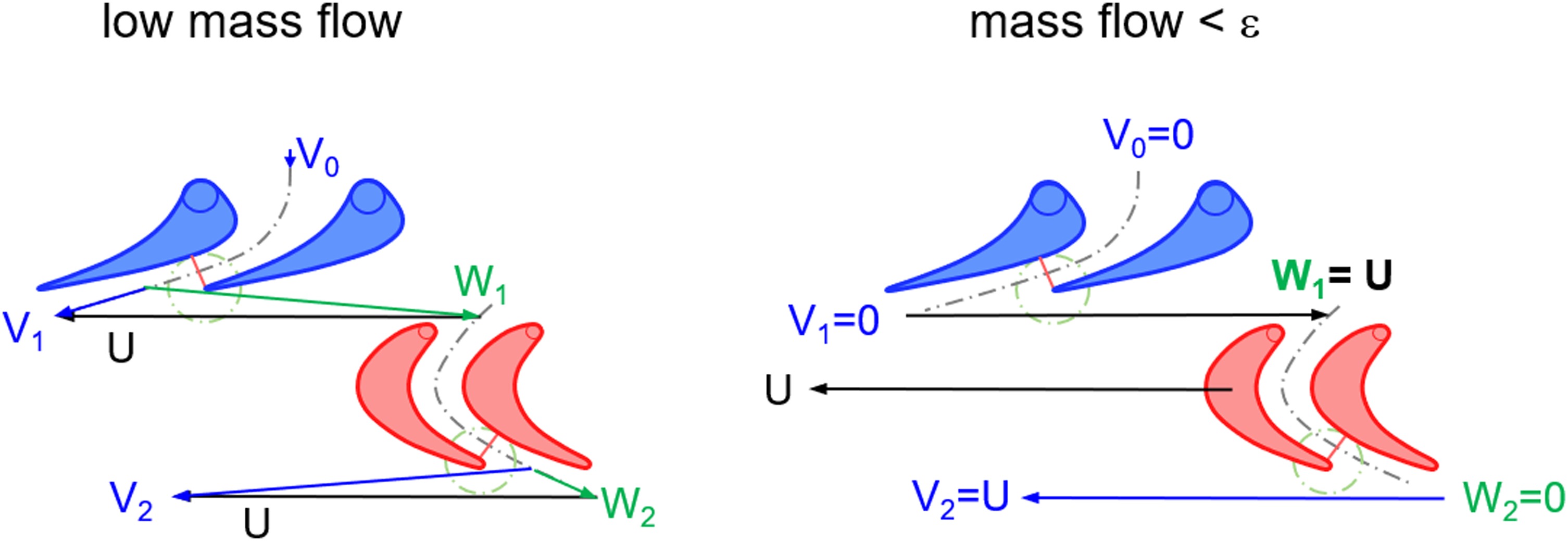
The enthalpy-entropy diagrams for the two low mass flow velocity triangles are shown in Figure 11. From the diagram on the right one can conclude that for the zero-flow case, the effective specific work Heff is twice as big as the isentropic specific work His since both W1 and V2 are equal to circumferential speed U.

Corrected isentropic work His/T1 is proportional to corrected speed squared:
His/T1 relates to pressure ratio:
Thus, pressure ratio relates to corrected speed:
Relating the true corrected speed to a reference value makes it easy to determine the constant in this equation because then the speed term equals unity. The difference between specific enthalpy for the temperatures T2,is and T1 for zero flow is W12/2 as the right part of Figure 11 shows.
Since W1 equals U (Figure 10) it holds that
The circumferential Mach number MU,ref at the map reference point needs to be estimated. The constant in Equation 7 follows from Equation 9:
Pressure ratio for any other corrected speed follows from
Flow at pressure ratio 1
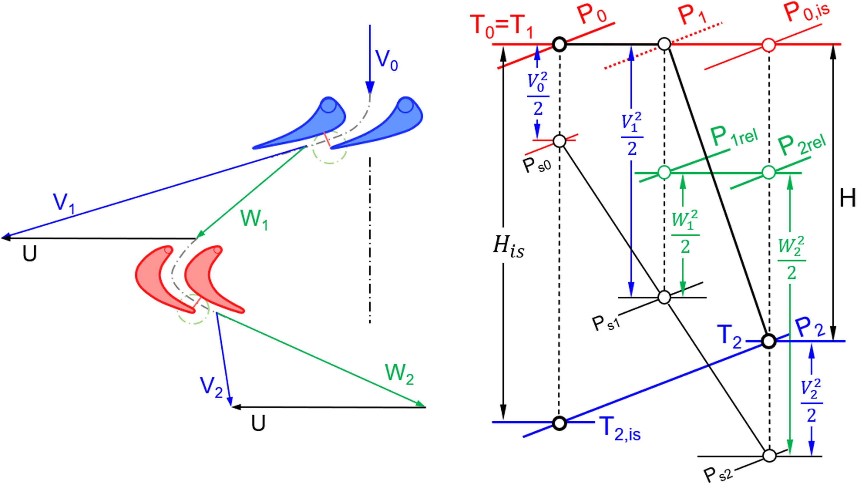
Figure 12 shows the velocity triangles and the enthalpy – entropy diagram for pressure ratio 1. The rotor entry triangle is symmetrical which makes the total temperature in the relative system T1,rel equal to the inlet temperature T1. The total pressure losses of the inlet guide vane P0 - P1,rel are compensated by the rotor, which works as a compressor.
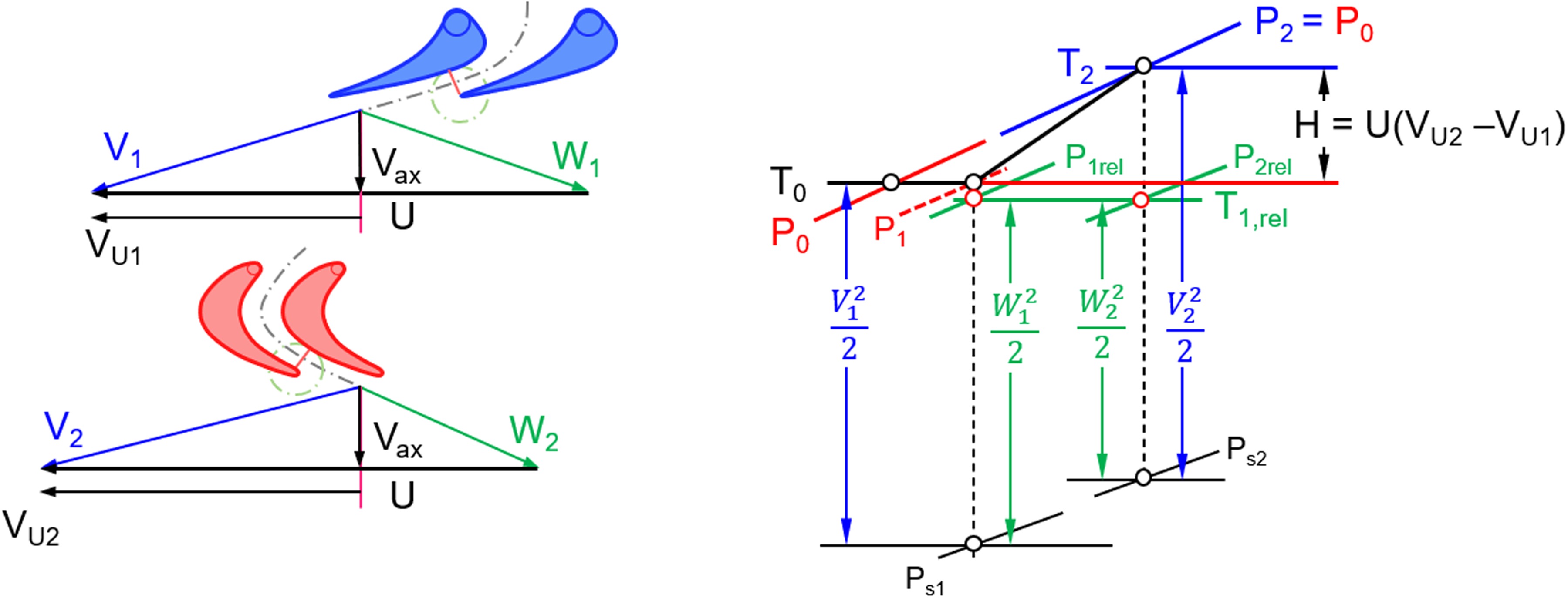
The shape of the velocity triangles remains the same when spool speed changes, the triangles remain similar. All enthalpy differences change in proportion to circumferential speed squared and mass flow changes in proportion to circumferential speed. Therefore, the pressure ratio 1 line is linear in a plot of flow vs. speed.
Application
The turbine map extension method described here is implemented in the most recent version of the program Smooth T. This software is a specialized plotting routine which helps a performance engineer generate smooth and meaningful lines through a cloud of measured or calculated data points. Many graphs show the measured data together with the lines in figures with physically meaningful parameters to allow checking whether the result makes sense or not.
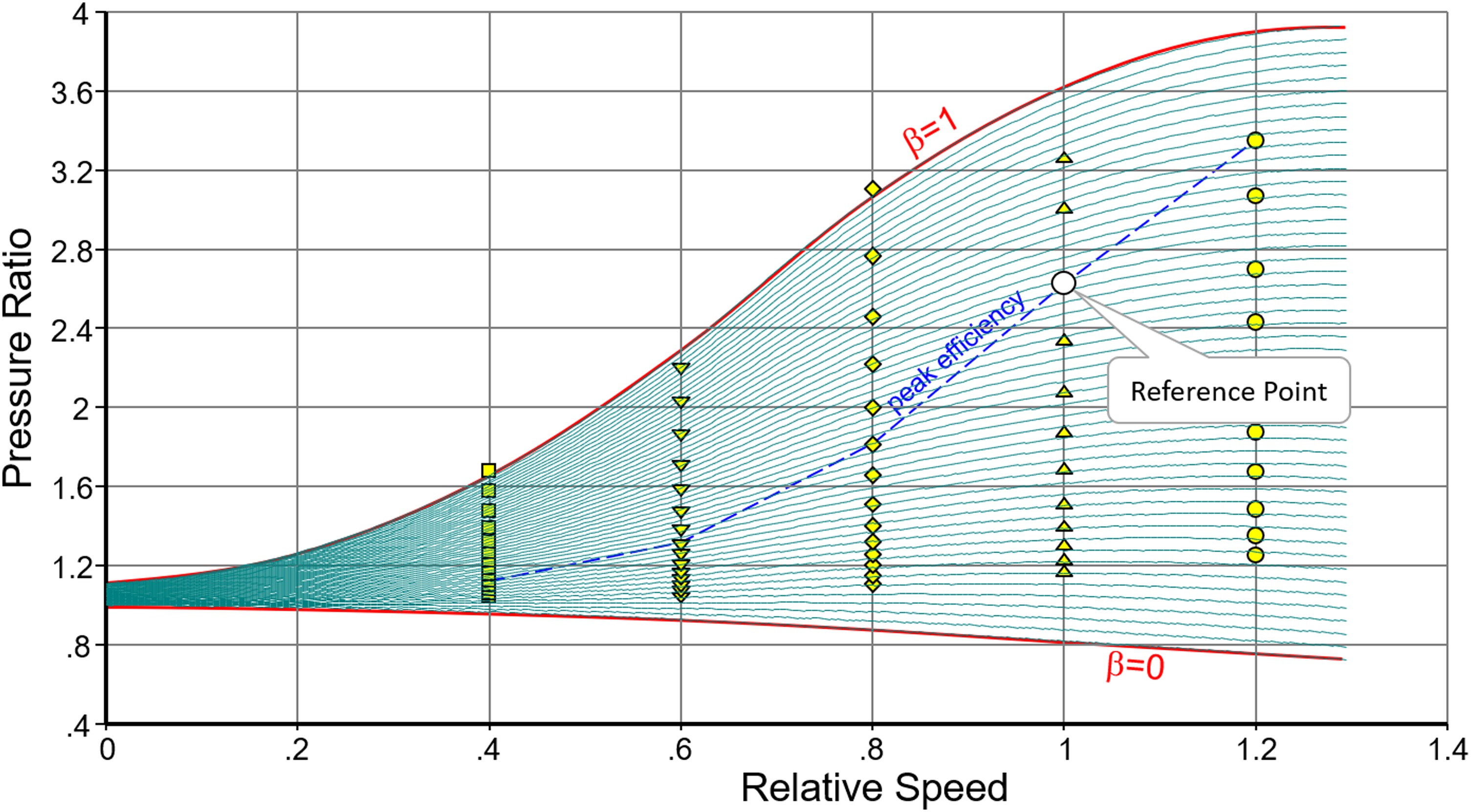
The efficiency contour lines in a pressure ratio – speed plot for a turbine define a landscape with a broad peak region at high speed (Figure 13). This high efficiency region becomes smaller in the mid speed range and deforms to a narrow ridge at low speed. Small differences in pressure ratio coincide with big changes in efficiency in this map region. Capturing the details of the efficiency ridge at low speed accurately would require a huge number of equally distributed pressure ratio grid points. Using a rectangular grid marked with the grey circles in Figure 13 would lead to severe accuracy problems in the low speed area. Moreover, we would have to store much useless data – especially in the region of high pressure ratios and low speed. We never need to know the turbine performance in that part of the map when we simulate standard gas turbine performance.
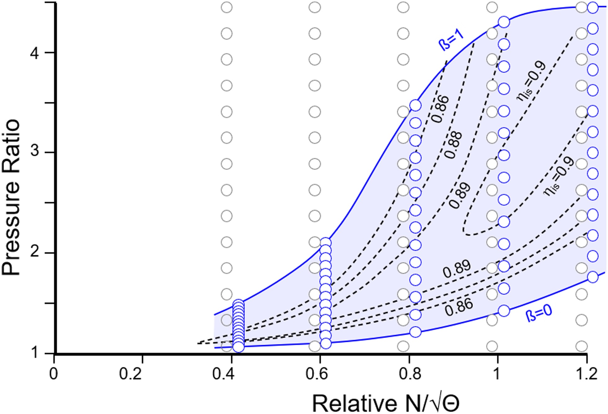
We can achieve high accuracy with a minimum number of grid points if we focus on the region of interest, which is the peak efficiency zone. The blue circles in in Figure 13 are distributed in such a way that we get adequate accuracy for any point of interest in the map. The blue circles are at the crossing between the speed lines with so-called ß-lines which serve as auxiliary coordinates for reading data from the map. (Kurzke and Halliwell 2018).
Baseline map
The turbine map shown previously in Figures 3, 4, 6 and 8 serves to illustrate the map extension method. This map is from a three-stage low pressure turbine designed for a business jet engine.
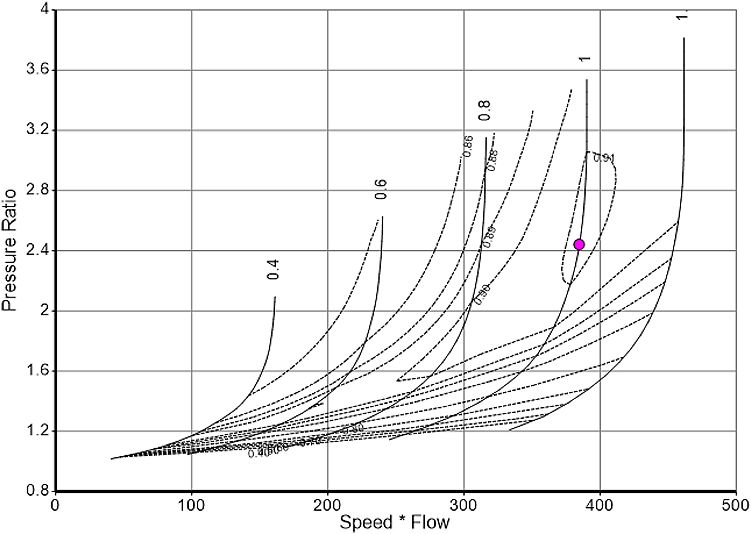
The map as shown in Figure 14 has been created using 30 ß-lines with the standard procedure described in the Smooth T manual. The ß-line grid encloses all the given data points. The ß-numbers (between 0 and 1) have no physical meaning. The map reference point is properly placed at the peak efficiency location of the speed line 1.
Extension to zero flow
A new ß-line grid is required for extending the map to zero flow. The upper ß-line (ß = 1) remains unchanged, the lower ß-line, however, will now get a physical meaning: it will represent zero-flow. This line passes through the origin (relative speed = 0, pressure ratio = 1) and bends downwards when speed increases. The shape of the zero-flow line is given by Equation 10 and is defined implicitly by the circumferential Mach number MU for relative speed 1.
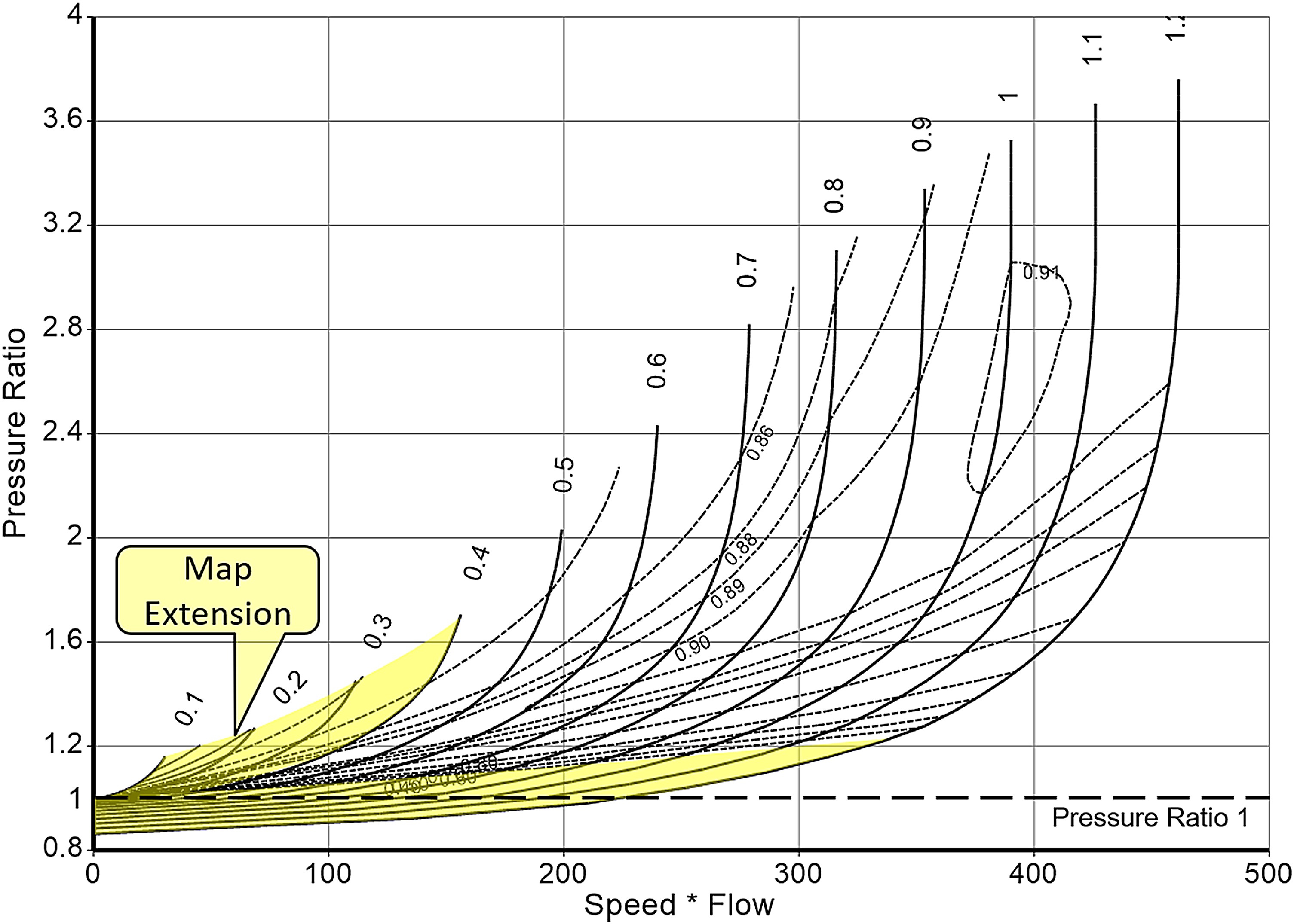
Note that the number of ß-lines needs to be increased because the pressure ratio range is bigger. 50 ß-lines have been used in Figure 15.
Start the map extension with a guess for the ß = 0 line by choosing MU = 0.5, for example. All the extended flow lines begin with mass flow zero on the ß = 0 line and approach the measured data points smoothly.
Modify the assumption for MU if the lines flow = f(pressure ratio) do not merge smoothly with the part of the line which is defined by measured data. Special attention should be paid to comparing the shape of the line for the lowest speed with that for zero speed.
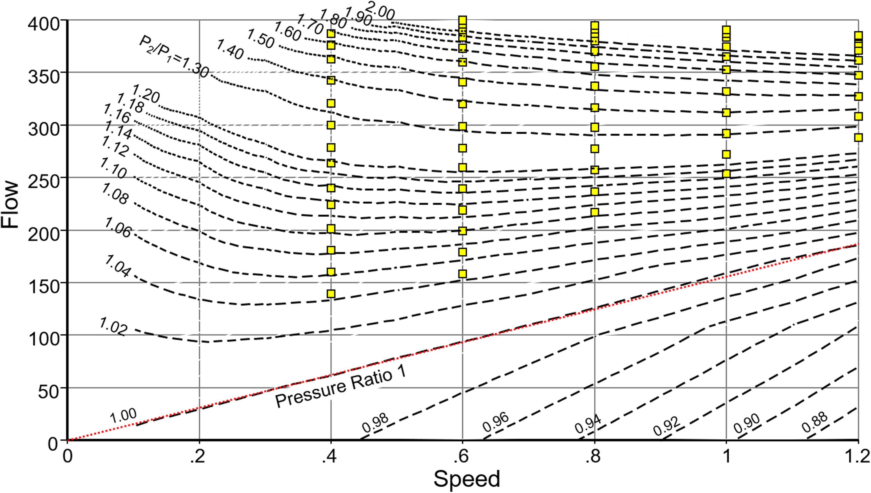
The discussion of Figure 12 lead to the conclusion that in a plot flow = f(speed) with contour lines for pressure ratio, the line 1.0 must be a straight line. As Figure 16 shows, this is true.
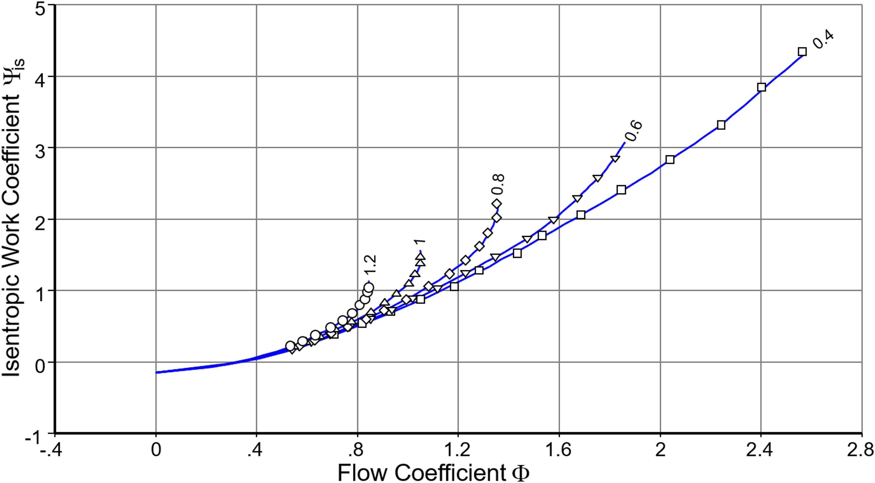
Also check the correlation between isentropic work coefficient and flow coefficient (Figure 17). All speed lines must collapse in the low flow coefficient region.
Next check if the torque/flow = f(flow) lines are straight in the region of low flow. That corresponds to low Mach number and is where incompressible flow theory is applicable. Figure 18 shows how the extended map looks now.
Equation 1 indicates that in incompressible flow the correlation between work and flow coefficients is linear and all lines collapse. Figure 19 shows that this is truly the case in our map example.
Extension to low speed
Extending the map to low speed uses the same ß-line grid as before. Add one speed line after the other and adapt the mass flow line first in such a way that it matches Figure 20 reasonably well.
Next check the torque/flow = f(flow) plot – in the beginning it will probably not look good. Correct the torque/flow lines in such a way that efficiency lines up with the other data in the plot efficiency = f(speed/jet velocity), as in Figure 6.
If it is not feasible to get both efficiency and torque/flow lines right, then the form of the function flow = f(pressure ratio) needs to be modified. Go back and modify the flow lines in such a way that the torque/flow lines have the desired shape.
To get all the correlations right requires only a few iterations. The final result of the map extension process is shown in Figures 20, 21 and 22.

Concluding remarks
The turbine map extension towards low mass flow is based on incompressible flow theory. The lower limit of the map is the zero-flow line – negative flow will not happen during aircraft engine start and windmilling.
The advantage of the current method over using map calculation programs is that no geometry information is needed. The accuracy of the result is more than adequate for starting and windmilling performance simulations.
The approach is implemented in the software Smooth T and has been applied successfully to many maps from the open literature. Starting and windmill relight simulations have been demonstrated with GasTurb. Deviations from full engine test data are expected due to uncertainties in the modeling of oil viscosity effects on gearbox drag and bearing losses. Also, combustor light up and efficiency immediately after ignition are in some degree random effects, and that makes an absolute agreement between model and reality improbable.