
Introduction
Reliable, detailed knowledge of the temperature profile across turbine blades is crucial in their operation and design, affecting their lifetime, efficiency and material selection. Internal cooling systems of turbine blades usually consist of a complicated labyrinth of channels and cavities, aimed towards intensifying heat transfer and distributing the coolant through the heat-loaded component. Film cooling is achieved through the formation of a thin layer of the cooling air uniformly distributed over the surface. This provides an insulating thermal barrier against the hot gas of the bulk flow. This is usually accomplished by a large amount of shape and flow optimized holes connecting the internal channels with the blade surface.
Despite relatively lower operating temperatures typically achieved in smaller engines, an excessive heat load may be comparatively challenging primarily due to their dimensions and compact designs. In addition, the gas generator turbine is often surrounded by an annular combustion chamber (CC) in so-called counter flow arrangement, which further constrains the heat transfer from the components.
The counter flow arrangement, with its high heat load factor, is used in gas generators in a production line of the První Brněnská Strojírna (PBS) engines represented by a turbojet TJ100, turboprop TP100 and finally a turboshaft TS100. These engines operate with an exit gas temperature around 900°C, which is considered a limit for uncooled rotating parts manufactured from nickel chrome super-alloys (e.g., Inconel 713 or 718).
Due to the relatively high turbine inlet temperatures and poor heat transfer, the vanes of the PBS gas generator suffer from extensive degradation occurring mainly in the region of the trailing edge. A novel concept of an active NGV cooling was proposed.
An initial study was conducted to develop a heat protecting system to avoid the erosion of the trailing edge caused by high thermal loads. The engine dimensions (maximum outer diameter about 270 mm) and its counter flow CC arrangement strongly limit practical design variants of a cooling system. The small size of the NGV further hindered the possibly to create a complex system of internal channels distributing the cooling air. Equally limiting were the allowable technical complexity and cost.
These constraints resulted in a simple concept of active fluid cooling with an internal vane cavity vented through seven cylindrical holes to the pressure side boundary layer, as shown in Figure 1. The cavity was to be supplied by the compressed air from the space between the CC and the outer diameter of the NGV shroud. Such a solution, however, required a redesign of the vane profile. Details about the redesign and the new geometry are addressed in the following section.
Figure 1.
A proposed concept of the NGV cooling.
The cooling air (blue arrow) enters the inner vane cavity and then is discharged through few cylindrical holes into the pressure side boundary layer (red arrow) thus forming a protective film on a portion of the vane surface downstream.
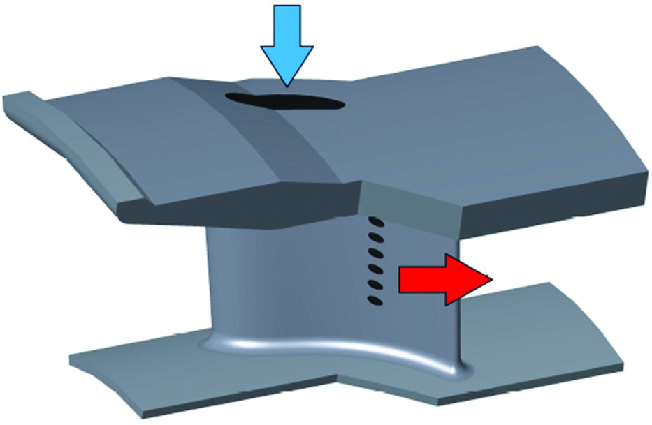
Two main effects were expected from the proposed cooling arrangement: a) heat transfer from the vane due to convection of air through the cavity and b) partial protection of the trailing edge region due to a film forming downstream the cooling holes.
In order to realize the cooling concept, the original vane profile had to be redesigned while maintaining the original flow parameters. The axial chord of the profile was enlarged and thickened in the front part to accommodate the internal cavity. As a result, the new NGV consists of only 17 vanes in comparison with 26 vanes of the original design.
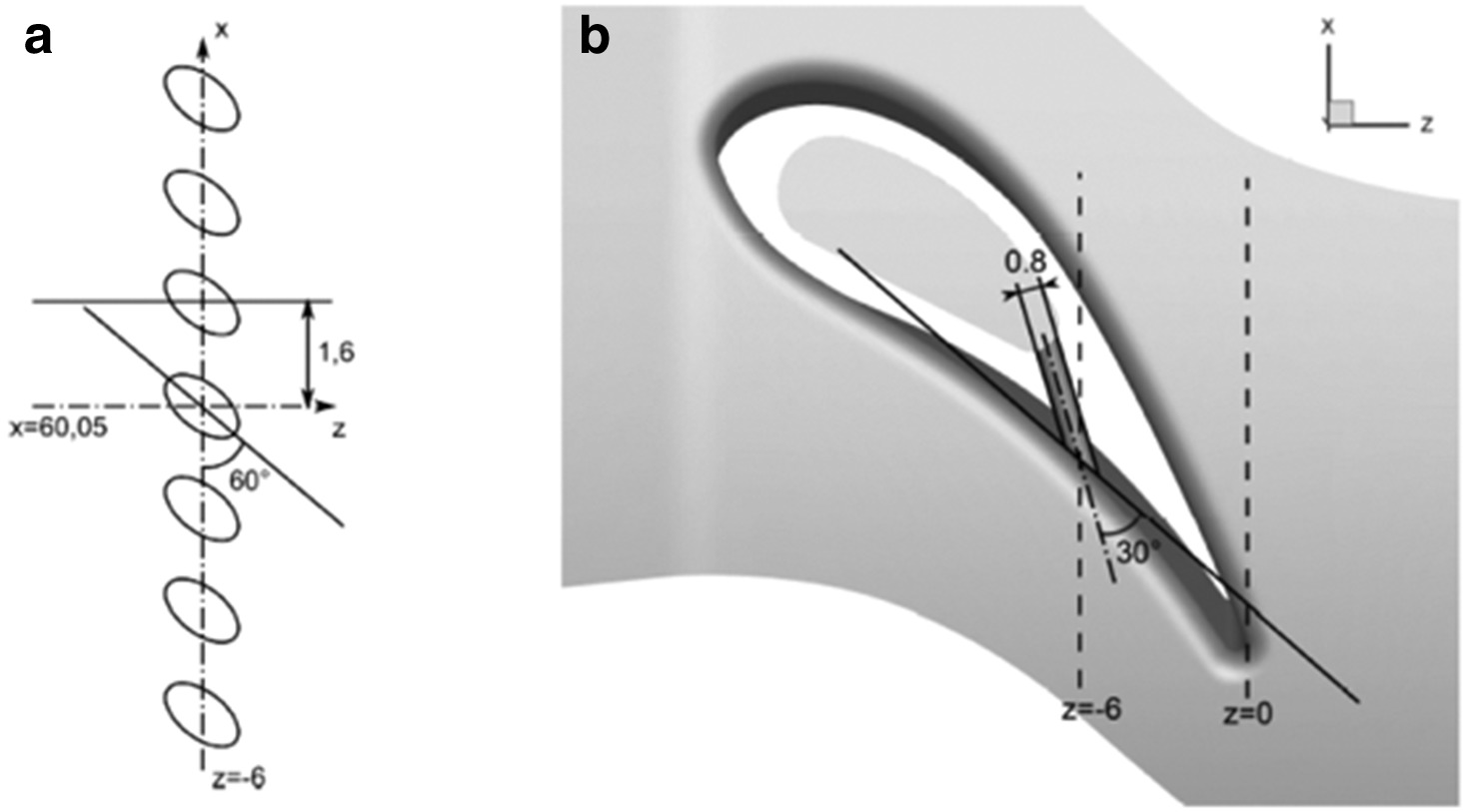
The tested cooling system consists of an oval shaped cavity, which goes through the thickest part of the vane and opens into an annular channel next to the shroud. Cold compressed air flows through this channel and is diverted before reaching the CC, which serves as a cooling medium. This cold air is brought from inside of the cavity to the surface of the pressure side of the vane by seven cylindrical holes. These holes are parallel to each other; each of them has a diameter of 0.8 mm and spaced two diameters apart. The central hole is positioned slightly above the mean radius of the wheel and the openings are located on the surface about one third of the vane from the trailing edge. The cooling channels were designed such that the middle one is inclined of 30° with respect to a tangent to the surface. The axes of the coolant channels are also tilted with respect to the machine axis with a compound angle of 30°. The configuration of the cooling channels is presented in Figure 2.
This investigation focused on evaluating this cooling design through the use of THPs and thermocouples. The thermocouples were used to obtain a temperature trace against time and to validate the THP readings at several locations as a novel measurement technology. Furthermore, the THP technology was used to increase the data resolution and provide full thermal maps across the surface, greatly expanding on the point measurements provided by the thermocouples.
Temperature sensor review
Conventional temperature measurement techniques provide temperatures online — values are obtained and recorded while the high temperature takes place. A widely used and well understood temperature measurement technique are thermocouples. These are based on the thermoelectric effect, causing an electric current between two different connected conductors to change as temperature varies. As a well-established technique, high accuracy can be achieved. However, only point readings are possible and the required wiring makes the implementation difficult, especially for rotating components. Moreover, the application of thermocouples is intrusive as they require direct contact to the measured component 18.
An alternative technique to measure temperature during operation is pyrometry. This technology measures the thermal radiation of a component without contact. Therefore, it requires optical access to the measured component during operation, causing technical difficulties; this often cannot be implemented or only allows measurement of limited regions of the component. Furthermore, exterior light and reflections from particles in the process gas can cause significant errors in the results. These errors can be compensated but the techniques to do that are rather time consuming 25, 8, 13, 19.
Another contactless temperature measurement technique is phosphor thermometry. Phosphor thermometry avoids the issue of stray light and reflection 9 but also requires visual access to the component and the need to install a laser to irradiate the component to generate the phosphorescence.
To avoid the requirement of access to the engine during operation, technologies have been developed to enable offline measurements. The most established offline measurement technique is temperature indicating paints or “thermal paints.” These paints are applied to the component and the component is run in the engine. During operation thermally induced chemical reactions take place which cause a permanent colour change 6. After operation the colour changes are interpreted by a trained technician under controlled light conditions 15. Thermal paints allow temperature mapping across a surface of a component but only with low resolution because the paints only provide colour changes in certain temperature ranges. Between these isotherms no temperature information is available and the analysis of the colour changes is subjective. In addition, dedicated short-term engine tests are required to allow for the low durability of the paints 4. Furthermore, some of the constituent materials and pigments of thermal paints are restricted under the EU REACH legislation European 20, such as chromium, cobalt and lead.
Other offline temperature measurement technologies rely on property changes of certain materials due to exposure to high temperatures, such as thermal crystals and templugs. Thermal crystals are irradiated before testing to generate lattice distortion. Thermal exposure reduces the distortion, which is measurable with X-ray diffraction very precisely 16, 3. Templugs change their hardness through heat exposure 17. Both techniques are intrusive because the material needs to be embedded in the component, and they only allow point measurements 2.
An alternative to the mentioned technologies are thermal history sensors, first proposed by 10. They consist of a ceramic material, doped with luminescent ions, which undergoes irreversible physical changes through temperature exposure. The changes can be measured by analysing the luminescent behaviour and correlated to temperature. The technology is capable of measuring temperatures between 150°C and 1,400°C 21, 22, 26. The doped ceramic material can either be applied directly through atmospheric plasma spraying (APS) or mixed with a binder into a non-toxic paint to generate a durable coating. This method allows 2D temperature mapping across a component’s surface with a precision of ±5°C and a spatial resolution of less than 3 mm proven up to 900°C 7. THPs were selected for measurement of the NGV.
Principles behind THP
Temperature measurements using THPs rely on the measurement of luminescent properties. While in the case of thermographic phosphors these changes are reversible 1, 14, in the case of offline THP they are permanent. This means that luminescent changes remain frozen into the structure and can be investigated after operation. These measurements can then be analysed to determine past thermal behaviour.
Two possible measurement methods for luminescent materials are based on intensity ratios or decay times. These luminescent parameters will undergo gradual non-reversible changes with temperature. The latter, lifetime decay, is usually preferred, as it requires simpler instrumentation and can be measured after operation to a higher precision. This means the technique is not dependent on signal intensity, and thus remains unaffected by polluted optics or soot deposits on the coatings.
Materials for this application are usually comprised of an oxide ceramic doped with an optically active ion such as a transition metal or rare-earth ion 5, 11, 23. For the lifetime decay method, the dopant ions are excited by irradiating the material with short laser pulses. The dopant ions absorb the energy then reemit it as light of a different wavelength. This emission arises due to relaxation transitions, and is characterised by long emission times, classifying it as phosphoresce. The intensity of this phosphorescent emission following excitation is characterised by I(t) and its behaviour with time can be fitted to a single exponential as follows:
In , I0 is the initial intensity, t is time and τ is the lifetime decay. Despite minor variations from a single exponential under certain conditions, very good fitting and results can be obtained by applying a Levenberg-Marquardt algorithm.
Excitation results in electrons being promoted to excited states from their ground state. The relaxation back to the ground state is termed relaxation, and can occur in one of two ways. Either radiative decay, which is accompanied by the release of photons, or non-radiative decay, which involves phonon emission. These are two competing mechanisms, and the probability of these occurring will determine the length of the decay time, τ, as shown in .
Where τ is the lifetime decay and PR and PNR are the probabilities of radiative and non-radiative decay respectively. In THPs, these probabilities depend on the gaps between energy levels. When the material is in the as-synthesised condition, it has a high number of defects and impurities left from the synthesis route, including H2O, CH2− or OH−. These act as phosphorescence quenchers, increasing the probability of non-radiative decay, PNR, and resulting in short decay times τ. As the temperature increases, these residual species are permanently removed, decreasing PNR and resulting in gradually increasing values of lifetime decay. This results in a gradual change in lifetime decay, τ, as function of exposure temperature, enabling the determination of past maximum exposure temperature by measuring the lifetime decay, following calibration.
Methodology
Considering the proposed number of the vanes (17), the test model resulted in an annular segment with only four blade to blade channels, i.e., three full vanes. Three alternative NGV segments were considered within the experimental campaign: a variant without cooling (NGV-NC), one with an internally delivered cooling (NGV-IC) and one with an externally delivered cooling (NGV-EC).
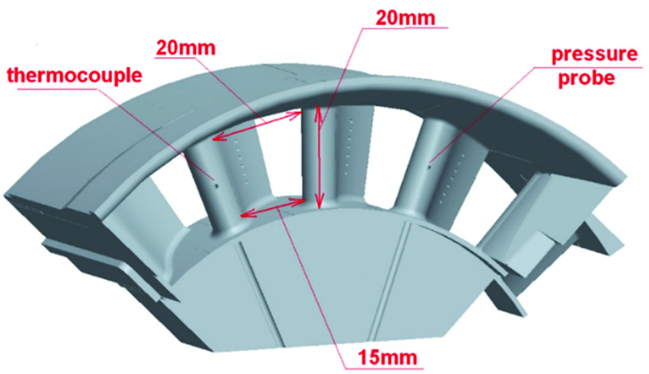
Only the NGV-IC was selected for the use with THPs. The NGV-IC variant, shown in Figure 3 represented a real engine configuration with three hollow vanes and seven cooling holes deployed on the pressure side of each vane. The variant utilized the coolant (mostly compressed air) from a space between the CC and the outer diameter of the NGV wheel. The cooling air was then returned back to the main flow through the cooling holes. The mass flow rate of the coolant was given by prescribed flow parameters and by an effective flow area of the cooling holes. The amount of the coolant was not measured directly.
NGV probe instrumentation
A shielded K-type thermocouple intended for measuring the total temperature (T0) of the exhaust gas was inserted into a channel prefabricated along one of the vane leading edges and fixed by a high-temperature resistant cement (Omega CC type), see Figure 3. The sensing end of the thermocouple was positioned at vane mid-height and connected with the hot gases through a drilled hole of 0.8 mm located in the vicinity of the stagnation point. The cavity of the probe was not ventilated.
A total pressure reading (P01) was performed by means of a stainless-steel tube of 1.2 mm inserted into a channel along the leading edge. It was again fixed inside the cavity by the high temperature cement. The tube end was connected to the medium through a drilled opening (0.8 mm) close to the stagnation point at the vane mid-height, see Figure 3. The cavity opening was not shielded.
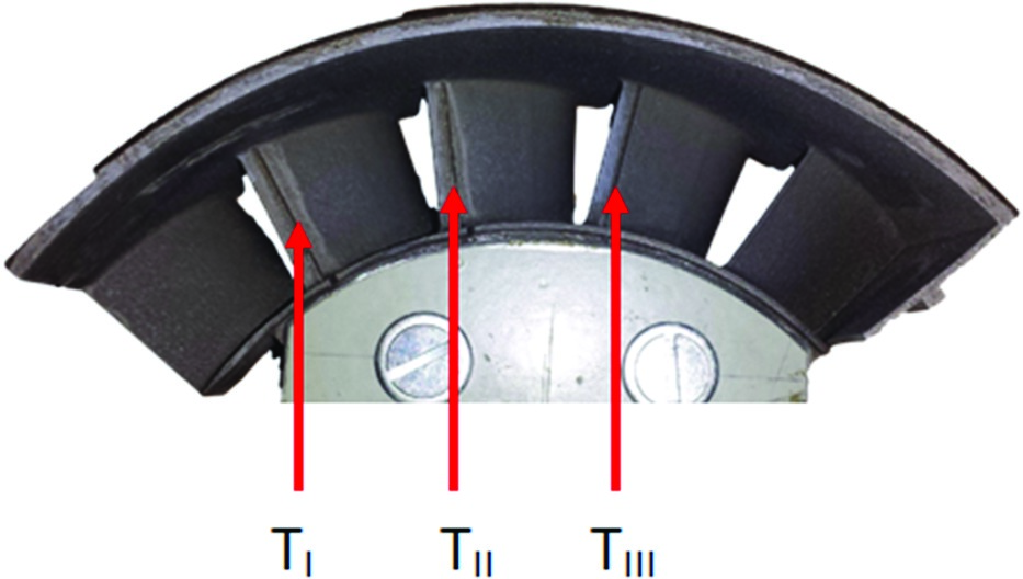
An average value of static pressure at the exit of the NGV was obtained by means of ten pressure taps (0.5 mm) deployed uniformly within two blade to blade passages. The distance of the pressure ports from the plane of the trailing edge was six millimeters. The vane metal temperature was monitored by means of three unshielded K-type thermocouples (∅0.5 mm) installed into the trailing edge region of the three individual vanes, as shown in Figure 4. They were flush-mounted into the pre-machined groves at vanes mid-height using a high temperature resistant cement. The thermal conductivity of the cement (15 W/m·K @ 260°C) was slightly higher to the used base material Inconel 718 (13 W/m·K @ 260°C).
Paint manufacture and application
THP is comprised of an oxide ceramic pigment mixed into a water-based binder. The ceramic pigment was synthesised using a standard sol-gel route as explained elsewhere 24, 12. Following synthesis, the powder quality was cross-checked through characterisation using X-ray diffraction. The paint was manufactured using an overhead stirrer by mixing the powder into a silicate water-based binder.
The component was prepared by masking any areas where paint was not desired. This included any surface outside the gas flow path and thermocouple and pressure probe locations. The holes in the leading edge were also covered. The component was then grit-blasted in order to remove any surface contaminants and to aid paint adherence. The sample was cleaned with acetone before painting. The paint was applied using a DeVilbiss gravity-fed spray gun. The paint was sprayed to an approximate thickness of 30 μm, which was monitored through the use of eddy current based thickness gauge. The paint was then cured in order to remove excess water and improve adhesion.
Engine testing
The test rig comprised three principal parts: a radial compressor (RC), a CC and the tested NGV segment. The amount of air supplied by the RC at the desired pressure was restricted by its working regime and, therefore, only a quarter segment of the CC was considered in the test rig.
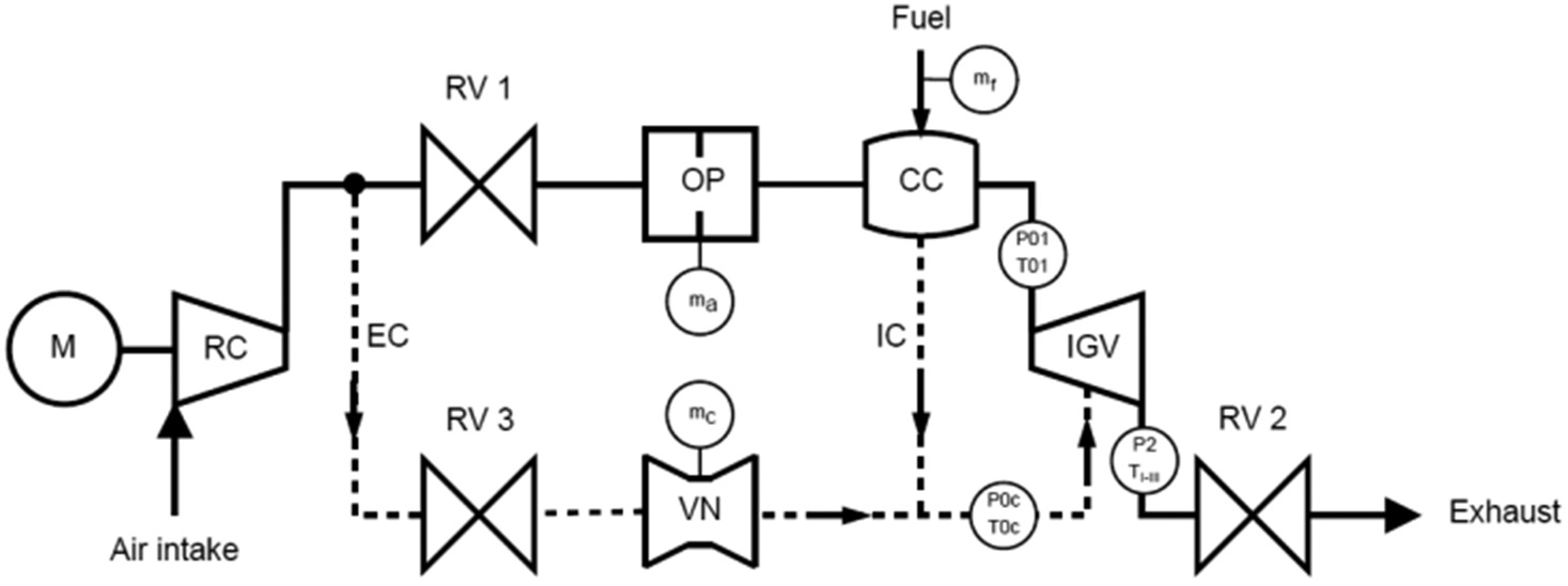
The desired mass flow and pressure ratios were achieved through the control of a compressor working regime and via two regulating valves RV1 and RV2 placed behind the compressors and NGV, respectively. An actual air mass flow rate delivered by the RC was measured by a calibrated orifice plate (OP) located before the CC. An entire amount of the mass flow rate across the NGV was thus given by a sum of the air and fuel mass flow rates. A scheme of the test rig with alternative cooling arrangements supplied with measured parameters is presented in Figure 5.
Figure 5.
A scheme of the test rig with two alternative cooling arrangements.
a) internally delivered coolant (IC) and b) externally delivered coolant (EC).
For this investigation, a “steady state” regime was reached for approximately six minutes where the NGV inlet temperature was measured to be approximately 850°C. The desired pressure drop on the vane was not reached. The outlet isentropic mach number (M2is) for this regime reached only around 0.6 instead of the intended M2is = 1, and therefore the full planned operation could not be achieved. However, it was still possible to perform measurements on the THP.
The paint remained adherent at all locations on the component. A photograph of the component after testing is shown in Figure 6. As expected, some colour variation was observed due to the thermal exposure. The colour variations provide an initial estimate of the temperature profile over the component. Darker areas, as seen at the base of the NGVs, indicate higher temperatures. Lighter areas, as seen on the shroud, indicate lower temperatures.

Instrumentation
The lifetime decay of the THP was measured using SCS’s portable opto-electronic system. It is comprised of a laser operating in pulsed mode, which is delivered to the sample surface through a fibre optic cable. The light reaches the sample, excites the luminescent pigments and results in corresponding light emission. This phosphorescence is collected into a different branch of the fibre optic cable, and delivered into a light detector after going through a bandpass filter. The resulting signal is then sampled by an acquisition card and fit to a single exponential decay, following in order to determine lifetime decay, τ.
Two different probes have been designed and are available to conduct measurements where there is restricted access to the painted surface. One probe, called “high resolution probe,” is held perpendicular to the surface and has a spot size of 0.5 mm. The other probe, called “90° probe,” is placed parallel to the surface and has a spot size of approximately 1.5 mm. A single measurement takes approximately five seconds.
Calibration
A calibration is needed in order to relate lifetime decay measurements to their corresponding temperatures. This requires samples with THP to be heated under controlled conditions to a known temperature for a fixed time. Calibration samples were produced at the same time as the test component by painting a set of 25 mm2 metallic coupons matching the material used for the NGV segment. The same paint and spraying methodology was followed for both. The coupons were then heat treated individually at a temperature between 350°C and 900°C for six minutes, in order to match the exposure time experienced by the component. Following the exposure, the samples were removed, cooled under atmospheric conditions and measured using the same instrumentation and settings used for the NGV segment.
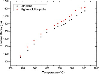
Each sample was used to construct one data point in the calibration curve, relating a particular temperature of exposure to the corresponding lifetime decay. Five repeat measurements were carried out per location. Two different probes were used to make the measurements on the NGV segment to overcome the limited access to the painted surfaces. The results of the calibration are plotted in Figure 7. The plots show the same trend, however there was an offset due to the different settings used for the different probe types. The calibration curve constructed was used to convert the measured lifetime decay values on the components into the corresponding temperature values. A linear interpolation between each neighbouring point pair was used in order to cover the full temperature range.
Figure 7.
The calibration data recorded from the samples. Different plots show the results from the two different probe types.
A single sample received the same heat treatment. The variation in measured temperature over each sample, therefore, gives an indication of the precision of the measurement. Two samples were measured at five different locations with five repeat measurements at each location. The standard deviation of all 25 measurements was used to estimate the precision of the temperature measurement. The estimated precision across the entire temperature range was below ±5°C.
Results and discussion
A number of preliminary tests were carried out with the NGV test rig setup outlined above. The primary vane regime can be described by a number of parameters. These are inlet temperature T0 = 850°C, total inlet pressure P01 = 476 481 Pa and by pressure drop: P2/P01 = 0.557 (M2is ≈ 1). The resulting thermocouple data is shown in Figure 9. The vanes show significantly different readings, which will be discussed later.
Figure 9.
Thermocouple data as function of THP test time.
The estimated time at temperature is approximately 6 min.
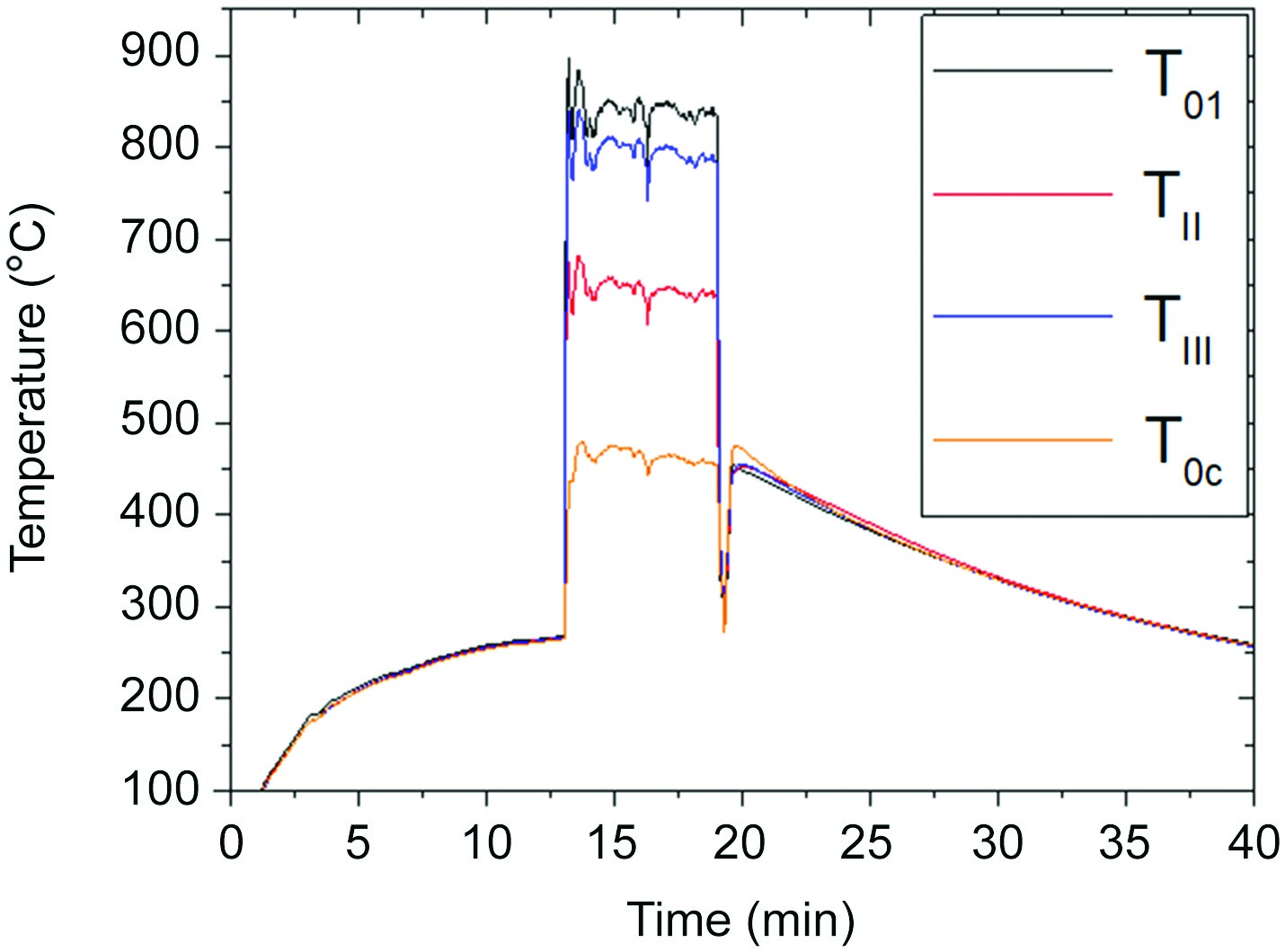
During the THP testing an unexpected fault resulted in lower pressure and Mach numbers than expected. TI could not be measured due to damage during the handling and coating application. The remaining thermocouple traces as a function of time are shown in Figure 9 (for probe locations see Figure 4). An approximately steady state regime was achieved for all thermocouples for 6 minutes, between 13 min and 19 min from the start of the test.
The mean, minimum and maximum temperature reached during the steady state for all thermocouples are shown in Table 1. The results show very good agreement between the THP test and the preliminary testing summarised in Figure 9. All thermocouples TI, TII and T0c compare favourably to past results. Therefore, despite the lack of measurement data for the TI thermocouple, its temperature was estimated to be in the same range as it was during the preliminary testing.
Table 1.
Mean, minimum and maximum temperature during steady state for all measured thermocouples.
| TC | Mean T (°C) | Minimum T (°C) | Maximum T (°C) |
|---|---|---|---|
| T01 | 840 | 778 | 896 |
| TII | 646 | 606 | 683 |
| TIII | 796 | 741 | 841 |
| T0C | 463 | 418 | 480 |
In both tests, the thermocouple recorded a large variation in temperature across different vanes. Such a difference may arise partially from the non-uniform heat conduction through the metal parts of the test rig. The relatively bigger auxiliary components of the rig connected to the NGV segment are maintained at considerably lower temperatures and therefore act as efficient heat sinks. This may explain the non-homogenous temperature distribution. Another reason for such phenomenon could be a non-uniform distribution of the inlet temperature due to irregularities in the CC. Generally, the observed temperature variance may be result of the non-periodicity of boundary conditions due to the non-annular NGV segments. Further information was sought through the measurement of THP.
The THP measurements were conducted using the read-out device in the SCS lab. Thirty repeat measurements were recorded at several different locations to determine the repeatability of the results. The standard deviation at a single location was within ±3°C. Measurements were taken across all areas where paint was applied. The focus of the following sections includes areas where thermocouple measurements were available for comparison. This enables the comparison between them and the validation of the THP technology. This is followed by a stronger emphasis on the capabilities of THP in providing detailed temperature maps across the surface of the component.
Pressure side
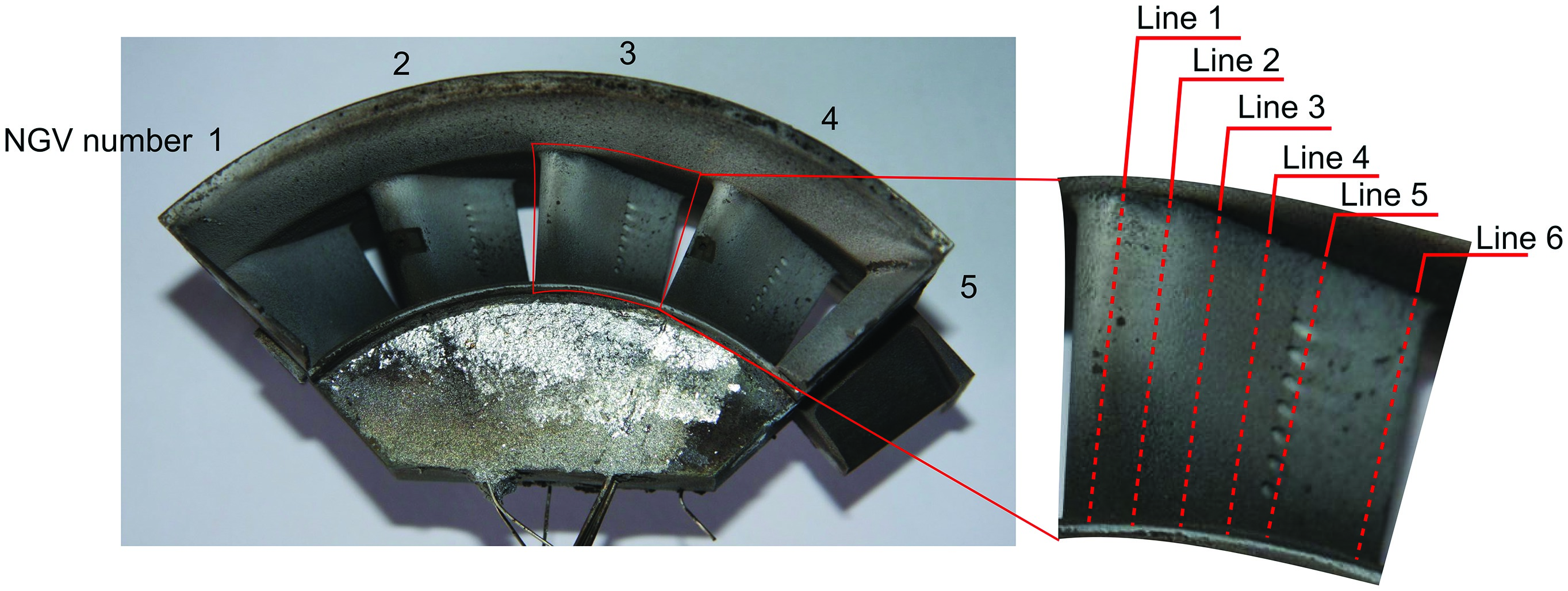
On the pressure side, each NGV was measured individually along six measurement lines as shown in Figure 10.
Figure 10.
The temperature measurements from the THP on the pressure side trailing edges of the three cooled NGVs (Line 6 in Figure 10).
To compare the results from the different NGVs the mean, minimum and maximum temperature from all the measurements on the pressure side are summarised in Table 2. The values in the table show there was a significant difference between the NGVs, as was observed in the thermocouple results. The mean temperature on the three cooled NGVs (NGVs 2–4) indicated NGV 2 was hottest, NGV 3 coolest and NGV 4 was intermediate. These results are consistent with the differences in temperature measured by the thermocouples at the trailing edges.
Table 2.
An overview of the measurements on the pressure sides of the NGVs.
| Measured T (°C) | NGV 1 | NGV 2 | NGV 3 | NGV 4 |
|---|---|---|---|---|
| Mean | 821 | 800 | 717 | 744 |
| Minimum | 688 | 684 | 547 | 603 |
| Maximum | 870 | 891 | 854 | 896 |
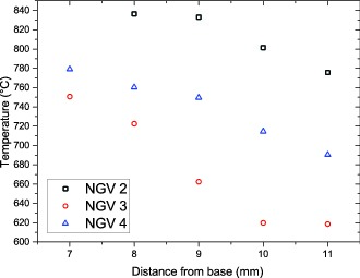
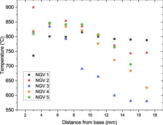
For further comparison, the results from THP at the trailing edges of the three NGVs with cooling holes are plotted in Figure 11. The plot shows the temperature profile was similar on all NGVs however the absolute temperature was different.
Figure 11.
The NGV segment showing the number assignment to each NGV and the six different measurement lines.
The paint was not applied at the same location as the thermocouples. Therefore, to directly compare the measurements from both techniques, the results were compared at the closest measured location on the THP to the thermocouples. This was at the mid-height of the trailing edge of the pressure side of each vane, where the thermocouple was located on the reverse side of the vane. The results of the comparison are provided in Table 3. The trend measured with THP is in very good agreement to the thermocouple readings. In all cases, the measured temperature is within the minimum-maximum ranges expressed in Table 1. The temperature on NGV (measured with TI) was taken from the preliminary test and is, therefore, only an estimate.
Table 3.
A comparison of the temperature measurement at the trailing edges for the THP and thermocouples.
| NGV | Measured THP temperature on pressure side (°C) | Mean TC temperature on suction side (°C) |
|---|---|---|
| 2 | 833 | 775Table 1 |
| 3 | 662 | 646 |
| 4 | 750 | 793 |
Suction side
A similar measurement procedure was carried out for the suction side. To compare the results from the different NGVs the mean, minimum and maximum temperature from all the measurements on the suction side are summarised in Table 4. The values in the table show the temperatures measured on NGV 1 and 5 were similar. These two vanes are the partial vanes at the edge of the NGV segment. The thermal exposure of these vanes were, therefore, expected to be similar.
Table 4.
Temperature measurements on the NGV suction sides.
| Measured T(°C) | NGV 1 | NGV 2 | NGV 3 | NGV 4 | NGV 5 |
|---|---|---|---|---|---|
| Mean | 799 | 789 | 664 | 743 | 798 |
| Minimum | 736 | 680 | 528 | 582 | 667 |
| Maximum | 887 | 900 | 834 | 843 | 884 |
As in the pressure side, the mean temperature measured with the THP on the three cooled NGVs indicates NGV 2 was hottest, NGV 3 coolest and NGV 4 was intermediate. These results are consistent with the differences in temperature measured by the thermocouples at the trailing edges. The results from the THP along a line adjacent to the thermocouple on all NGVs are plotted in Figure 12 for a further comparison. The plot shows the temperature profile was similar on all NGVs except NGV 1. This observation may be expected because of the different boundary conditions and geometry of NGV 1 compared to the other NGVs. The temperature decreased towards the shroud on NGV 2–5. The absolute temperature of the NGVs was different as stated earlier. The plot shows that NGV 3 was clearly cooler than the others, and NGV 2 was generally hotter than the rest.
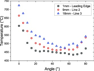
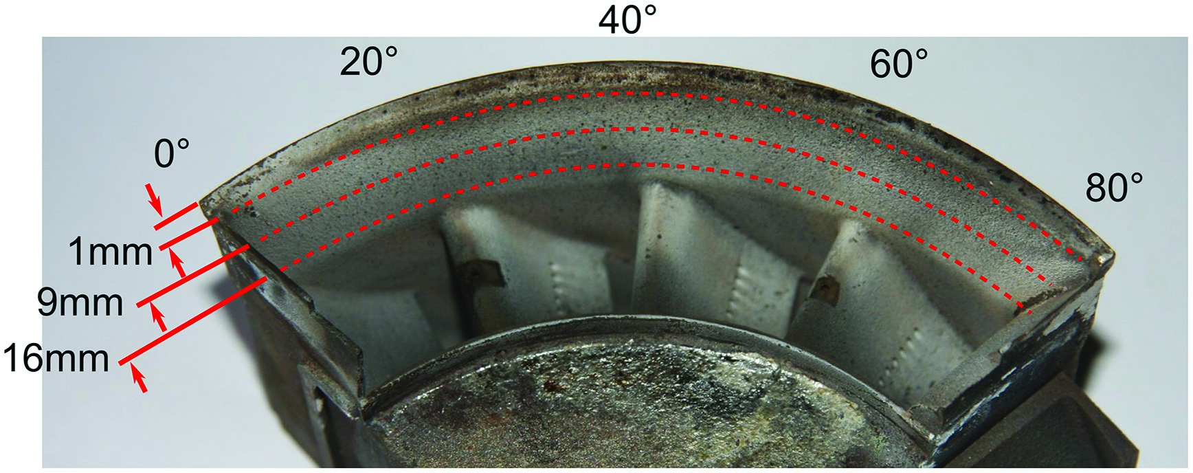
Shroud upstream
Measurements were recorded on the THP along three measurement lines as indicated in Figure 13. A measurement was taken every 5° around the circumference of the shroud. The results of the measurements are plotted in Figure 14. The temperature profile across all three measurement lines was similar. The temperature decreased from the left side and the temperature gradient appears to be similar. The temperature increased towards the leading edge of the NGVs. The temperature difference varied between 31°C and 120°C. Furthermore, the temperature increased by 30°C–50°C towards the right side (80°) on all measurement lines.
Figure 14.
The temperature measurements on the shroud upstream at the three different measurement lines as shown in Figure 13.
Shroud downstream
The shroud downstream was measured along four measurement lines, shown in Figure 15. A measurement was taken every 5° around the circumference of the shroud. The notation of the angles is anti-clockwise to match the angular values to the shroud upstream.

The results of the measurements on the shroud downstream are plotted in Figure 16. The figure shows that the temperature increased on all measurement lines to a maximum at a rotational angle of 20–40°. This indicated that there was a band of higher temperature across the shroud surface.
Figure 16.
The temperature measurements on the shroud downstream at the four different measurement lines.
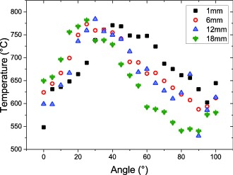
The temperature variation was greater closer to the NGVs. All measurement lines follow a similar trend, except the line at 12 mm between 80° and 95°. At this location there was a wide fluctuation in the temperature measurements in a short space. Here the measurements were made at the repair on the component, therefore, there was a different substrate material. The change in material may be the cause of this fluctuation in the temperature measurements, either due a change in temperature due to the different material or due to an interaction between the paint and the substrate material.
The results plotted in Figure 13 are represented as a contour plot in Figure 17. The plot clearly shows the temperature variation over the surface of the shroud downstream. The figure clearly shows a higher temperature region which corresponds to the gas stream exiting between NGV 1 and 2. This observation indicates the gas stream was hotter over NGV 2, which correlates to the temperature measurements on the pressure and suction side of the NGVs. This thermal map demonstrates the capabilities of THPs, which enabled the generation of a detailed temperature map across the component surface over quite a small area. The results shown agree with observations made of both the pressure and suction side. While they reveal the same trend as the thermocouples (i.e., NGV2 was the hottest), these results expand on that information and accurately reveal the precise gas stream path.
Figure 17.
The temperature measurements on the shroud downstream represented as a contour plot where the contours are at every 20°C.

In general, the presented results proved the feasibility of the proposed cooling concept adopted for a small turbine engine. An extended lifespan of the cooled NGV may be expected while maintaining a relatively high temperature at the inlet. Additional tests on a real engine should be performed in order to verify the concept with more realistic boundary conditions (in terms of heat transfer) and with a longer operational period. Despite the attained drop of the NGV metal temperature, the main effort in dealing with the temperature degradation of hot engine parts should be focused on achieving stable working conditions of the CC, thus producing a homogenous temperature field without any hot spots and spatial and temporal irregularities.
Conclusions
A novel concept of an active NGV cooling was proposed. In order to assess its feasibility and effect on vane temperatures, a test was devised involving THP and thermocouples. THPs are a novel temperature measurement technique capable of providing accurate objective past temperature information. THP was applied to a NGV segment and samples of the same material. The engine was with the NGV segment was operated, reaching a constant temperature for approximately six minutes.
The painted tiles of the same material as the blades were used to produce a dedicated calibration data set for this test. The tiles were heated individually for six minutes at a range of temperatures. After cooling, they were measured to generate the calibration of lifetime decay and temperature. The results on the tiles indicated a precision of the measurement of ±5°C.
The paint remained adherent to the complete component during testing. Nearly 400 measurement points were obtained for the pressure and suctions sides, as well as the shroud downstream and upstream. Thermocouple data revealed a significant difference in temperature between vanes. This was attributed partly to the non-uniform heat conduction through the metal parts of the test rig and partly to non-uniform heat distribution in the exhaust from the combustor. The results obtained through the THP supported the thermocouple readings and were able to further provide extensive thermal maps across surfaces including the shroud downstream, providing a clear indication of the hot gas stream path. The results showed that the THP extends the limited information from thermocouples to provide a more complete view of the thermal processes on the component.