
Introduction
Most gas turbine performance calculations concentrate on the operation between idle and maximum power. For turbofans, the lowest corrected spool speed considered for that purpose is around 60% for the gas generator compressor and 30% for the low-pressure compressor. If a compressor rig is part of an engine development program, its speed range is usually limited to that encountered between idle and full power. All the usual issues of interest to performance engineers can be addressed by using the data this imparts. However, when extraordinary operating conditions are to be considered – like engine starting and windmilling – compressor maps which include the sub-idle region are indispensable.
If the compressor geometry is known in sufficient detail, it is feasible to calculate at least part of the sub-idle performance. However, it is difficult to make the computation agree with the rig results for the lowest measured speed. If the required input data for running a map calculation program are not available, then the only remaining option is to extend the existing map by some means.
Prediction of compressor performance for speed zero is simpler than for any other condition since no energy transfer is involved. However, as soon as the speed is larger than zero, the efficiency of the compression process comes into play, and that creates problems in the region where pressure ratio is near to unity. The map extension methodology described in the following addresses these problems and creates a consistent and precise description of the compressor performance even for speeds as low as 1%.
The behaviour of jet engines at extreme operating conditions has been of interest for a long time. Sobolewski and Farley (1951) wrote in the introduction to their report about jet engine windmilling tests with power offtake:
There is a trend in modern aircraft design to depend increasingly on accessory power for safe flight. In the event of combustion blowout or other engine failure, the time sufficient power is available for rapid, sure operation of landing gear, flaps, etc may be critical.
The available duration of auxiliary power from engine driven accessories in the event of combustion flame-out or other engine failure is considered for flight Mach numbers from 0.19 to 1.06 and altitudes between 5.000 and 50.000 ft. The problem exists also with today’s aircraft.
Shou (1980) describes two empirical methods for calculating windmilling of turbojet engines and discusses how to “solve the simultaneous equations of all component characteristics”. He models the compressor performance with equations valid for windmilling, while contemporary gas turbine performance programs use full compressor maps.
The comprehensive literature review of Ferrand et al. (2018) comments on various methods for the extrapolation of compressor maps to sub-idle speeds. Such a process usually uses similarity laws for incompressible flow and begins with the data from the lowest known speed. The quality of the extrapolation may be improved by accounting for compressibility effects (Gaudet and Gauthier, 2007; Wang et al., 2015). An experimental validation of this extrapolation method was published by Hönle et al. (2013).
In recent years researchers from Cranfield University, UK have published several papers addressing the sub-idle and windmilling performance of compressors, see Aslanidou et al. (2010), Zachos et al. (2011), Grech (2013) and Ferrer-Vidal et al. (2018). In 2021 Ferrer-Vidal published another paper which begins with an extensive literature review. Some of his conclusions are difficult to understand. He states, for example, that the method described by Riegler et al. (2001) produced inconsistent maps due to the amount of user judgement and manipulation required. Riegler, however, shows in Section 3.2.3 and Figure 1 that generating maps graphically can indeed be valid. The engineering judgement of three different people resulted in maximum deviations between their results and the measured inlet corrected flows respectively pressure ratios of about 0.7 percent. By the way, Riegler and his colleagues used version 7 of the well-known Smooth C program for their work.
The method described by Ferrer-Vidal in his 2021 paper provides a physics-based approach to generate maps down to zero speed based on mean-line geometry. It builds on the method presented by Zachos et al. (2011) and improves it, by defining a calculated torque-free characteristic in addition to a calculated locked rotor line. The method generates consistent maps without user judgement affecting the outcome. A sensitivity analysis with respect to inaccuracies is included in the underlying mean-line method.
The origin of a compressor performance map is either a rig test or a calculation. The generated data can be used for training a neural network [see Ghorbanian and Gholamrezaei (2007), Gholamrezaei and Ghorbanian (2010) or Lory and Orkisz (2022)] or for generating a mathematical model consisting of ordinary polynomials (Li et al., 2018), Chebyshev polynomials (Zagorowska and Thornhill, 2017), ellipses (Tsoutsanis et al., 2012, 2014) or Bezier curves (Shuang et al., 2021). All these approaches require significant pre-processing before a satisfactory compressor map is ready for use in a performance program. It is much less time consuming to convert available data into simple look-up tables.
Usually, compressor performance is presented as a graph of pressure ratio P2/P1 versus corrected flow W with corrected speed N as parameter, enhanced with lines of constant efficiency. Reading data from such a graph is not trivial because the shape of the lines P2/P1 = f(W) for constant N varies with speed. In the mid-map region, pressure ratio always decreases when flow increases. If speed is low, however, it can happen that – starting from the surge point – pressure ratio first increases, reaches a maximum and then decreases again. Two mass flows for a given pressure ratio can exist on such a speed line.
If mass flow is the known input, we can determine the pressure ratio easily on a speed line. However, if the speed is sufficiently high, then the lower pressure ratio part of a speed line is vertical. In this part of a speed line, we cannot determine pressure ratio from mass flow. So, it is possible to locate a point everywhere in the map neither with given speed and pressure ratio nor with given speed and mass flow. We must look for another way to locate the compressor operating point in the map.
The solution to this map reading problem is the introduction of auxiliary coordinates – lines which are essentially parallel to the surge line. Instead of one look-up table P2/P1 = f (N, W) we use two tables P2/P1 = f (N, Z) and W = f (N, Z). Speed N and the auxiliary coordinate Z define the compressor operating point unambiguously.
Koenig and Fishbach (1972) defined Z as relative pressure ratio along a speed line. Z = 0 corresponds to the lowest pressure ratio on a speed line and Z = 1 to the highest, i.e., the surge pressure ratio. Thus Z = 1 has a physical meaning, but Z = 0 has not because the lower end of a speed line is an arbitrary choice. Note also that this definition of Z is not suited for speed lines where the surge pressure ratio does not correspond to the maximum pressure ratio.
Instead of Z one can use other correlations as auxiliary coordinates, for example a set of straight lines through the origin {P2/P1 = 0, W = 0}, parabolas or other curves. The auxiliary coordinates need not have a physical meaning, their main purpose being the unambiguous evaluation of the compressor map look-up tables, but it is desirable that they do. One can use lines of constant surge margin, compressor exit corrected flow, work coefficient or the distance from the peak efficiency line (the backbone) of the map as described by Sethi et al. (2013), for example.
The data are stored in rectangular look-up tables in which every single value should be meaningful. However, that is only the case if the range of the auxiliary coordinate values is independent of speed. This condition is usually not fulfilled when a physically meaningful quantity is selected as auxiliary coordinate.
A generally applicable auxiliary coordinate system must be suited for maps from all sorts of compressors, as there are axial and radial, single, and multistage, as well as compressors with or without variable guide vanes. The following approach has been in use since the early 1990’s at MTU Aero Engines. Two parabolas enclose the map, whereby the lower parabola is marked as β = 0 and the upper parabola as β = 1. Typically, 20–30 equally spaced parabolas are placed between the two limiting β-lines.
The author of this paper has published studies on compressor map modelling with β-lines in the years 1996, 2011, 2014 and 2019 (Kurzke 1996, 2011, 2014, 2019). In Kurzke (2012) he presented a collection of 59 compressor maps ready for use in gas turbine performance programs. Together, these publications prove that using parabolic β-lines is a universally applicable auxiliary coordinate system.
In his most recent paper dealing with compressor maps the author (2019) describes a method for extending maps to the sub-idle region, as needed for simulating starting and windmilling. The method works reasonably well down to about 10% spool speed; creating lines for lower speeds is cumbersome, however. This paper describes an enhancement of the method which can easily create lines for speeds down to 1%.
Theory
The smallest area within the flow-path of a compressor is the throat area in the exit guide vane (EGV). Incompressible flow prevails everywhere in the compressor when the exit guide vane throat Mach number is less than say 0.4. Its precise calculation would require knowledge of the detailed geometry as well as the flow direction downstream of the last rotor. However, knowing an approximate EGV throat Mach number is sufficient to identify the incompressible flow limiting line in the map. Kurzke (2019) describes how to estimate the EGV throat Mach number everywhere in the map. In the incompressible flow region, the following non-dimensional relationships between work, flow and torque are a big help for the map extension to low speed.
Work and flow coefficient
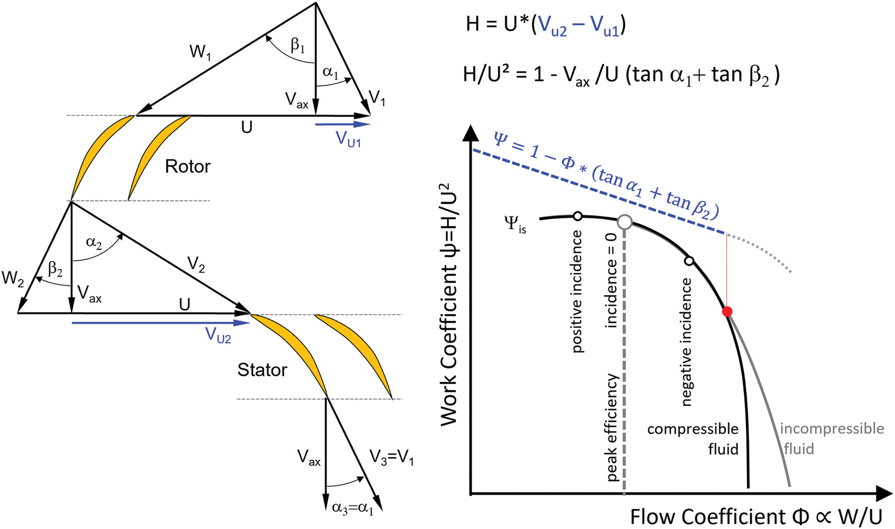
If we consider the form of the ψ − Φ relationship for a single stage compressor with symmetrical velocity triangles in simple terms, we can conclude from Figure 1 that ψ is a linear function of Φ. This follows from the fact that the flow leaves a blade or vane row in the direction given by the trailing edge geometry.
Work input H done on the air by the compressor is represented by a straight line when plotted as Ψ against Φ, whereas work output His calculated from pressure ratio is vastly different. The losses in the compression process, described by efficiency η = His/H and quantified by the difference H − Hi, are smallest at the peak efficiency point.
The only prerequisite for the validity of Equation 1 is that the flow direction downstream of the blades and vanes is imposed by their geometry. In an incompressible fluid (constant density) there is only one curve for ψis = f(Φ) and it is valid for any speed.
Torque
Compressor power can be expressed as the product of flow W and specific work H, as well as the product of angular speed ω and torque Trq:
Rearrangement and insertion of Equation 1 yields
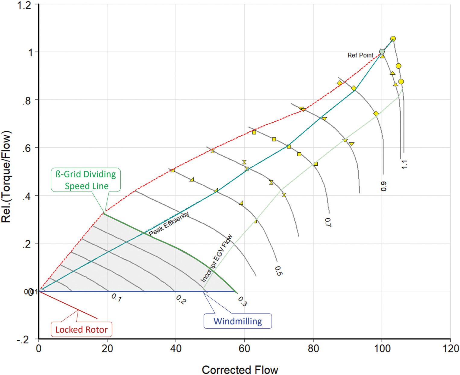
This equation is valid where flow velocity Vax is proportional to mass flow W – in other words, for incompressible flow. Under this condition, Trq/W2 is a linear function of 1/Φ and, for a given circumferential speed U, Trq/W is a linear function of W:
The partial derivative ∂(Trq/W)/∂W – the slope of the line Trq/W = f(W) – is independent of the circumferential speed U. The slope of the line H = f(W) is also of interest; it can be derived from Equation 5 which combines Equations 2 and 4:
The partial derivative ∂H/∂W – the slope of the line H = f(W) – is a linear function of spool speed.
The zero-speed line
The zero-speed line has some special properties which cannot be described by a ψ − Φ correlation. However, we know quite a lot about the zero-speed line.
No work is done (specific work H is zero) when the compressor does not rotate.
In the incompressible flow region, the P2/P1 = f(W) line is a parabola, since it describes the flow through a locked rotor as being like that through a pipe with obstacles and friction
We have concluded from Equation 4 that the slope of the Trq/W = f(W) lines is independent of speed in the subsonic region of the map.
We know that in the incompressible flow region of the map, the peak efficiency ηpeak always occurs at the same value of Φ or Ψ.
Thus (Trq/W)peak eff is proportional to W for a given value of Φpeak eff. Since all peak efficiency points happen to be at the same flow coefficient Φpeak eff, they all must be on a straight line from the peak efficiency point on a speed line to the origin {W = 0; Trq/W = 0}.
Application
Kurzke (2019) has explained how a map can be extended down to 10% speed. The following describes how the quality of this map extension methodology can be improved for speeds less than 30% and how accurate lines for speeds down to 1% can be generated with little effort. The measured map published by Hatch and Bernatowicz (1957) serves as an example because windmilling test data from the same compressor are available (Hatch, 1958). So, it is feasible to compare the results of the map extension generated by Smooth C with measurements.
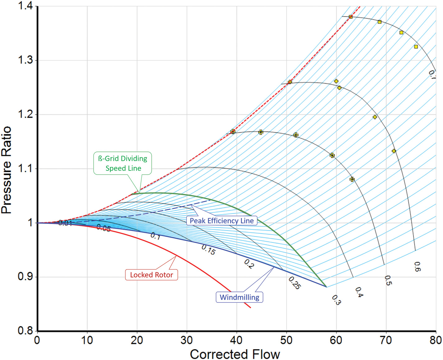
All the theory presented above is valid only in the map region where incompressible flow prevails. Its boundary can be derived by considering the Mach number in the exit guide vane, as explained by Kurzke (2019). In Figure 2 the incompressible flow region (above the line with exit guide vane EGV Mach number 0.4) is in colour.
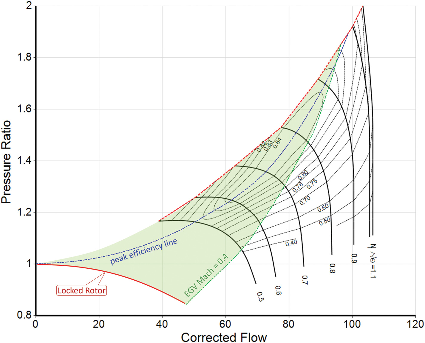
The peak efficiency line – also known as the backbone of the map – is highlighted. Theory says that within the incompressible flow region the peak efficiency line is a parabolic line with constant ψ and Φ.
The β-line grid
Generating a smooth representation of the available data is the first step in the map extension process. We introduce β-lines as auxiliary coordinates needed for reading the map unambiguously in a performance program; generally, they have no physical meaning. The β-lines in Smooth C consist of a set of parabolas with parameter values from 0 to 1. The compressor map output is restricted by the lower parabola (labelled β = 0) and the upper parabola (labelled β = 1).
Figure 3 shows a typical β-line grid suited for simulating the normal operating range of a gas turbine compressor between idle and full power. This grid is not convenient for simulating starting and windmilling because the region below the locked rotor line is irrelevant for performance calculations. Most of the region between the locked rotor and the windmilling line is not even needed for that purpose.
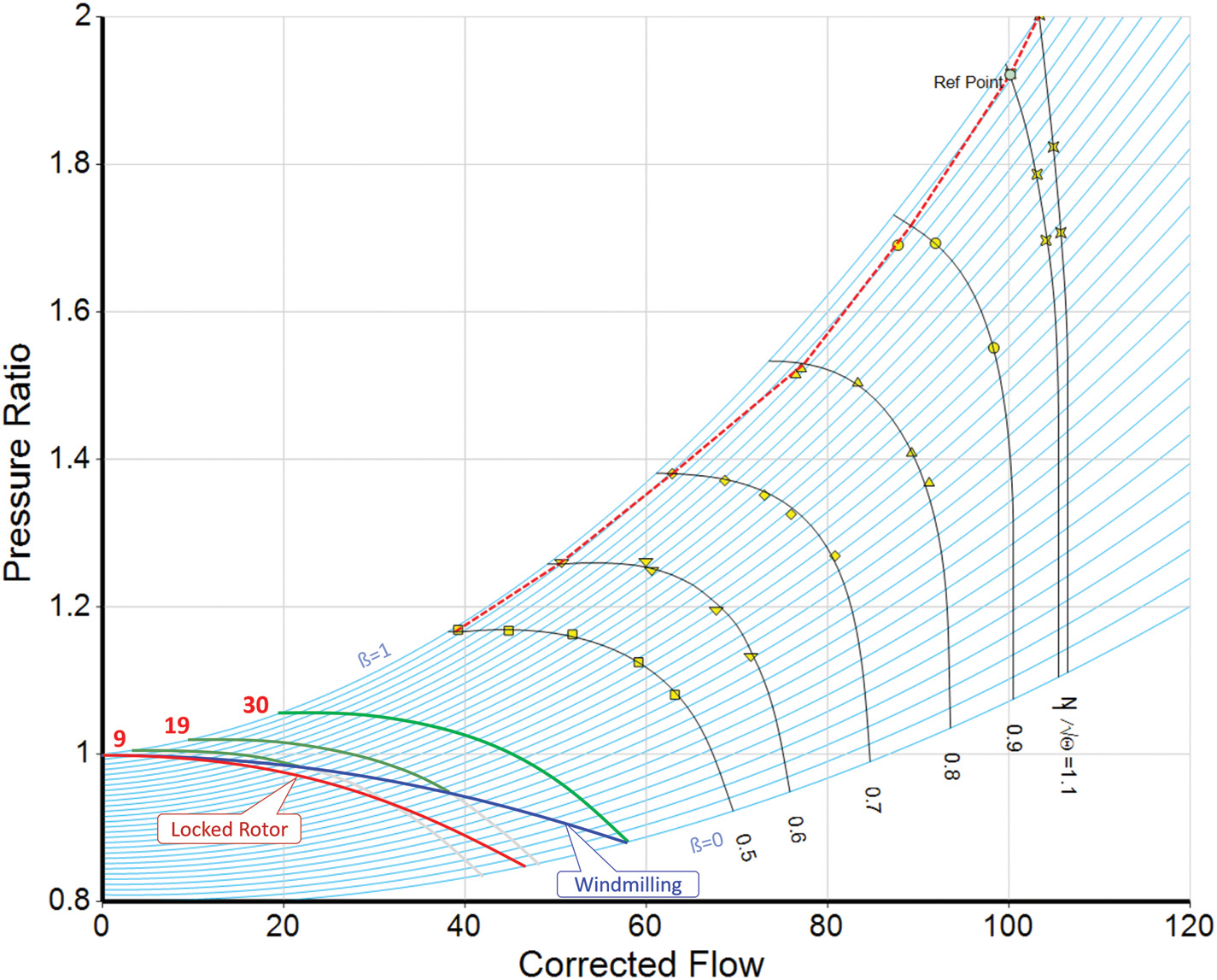
The problem with this β-line grid is that the number of useful β-values in the performance map decreases when moving along the windmilling line from high to low mass flow. On a speed-line starting at the high mass flow end of the windmilling line, all 30 β-values are associated with meaningful data. For a speed line which crosses the windmilling line at a flow rate of 42, only the data for 19 β-values make sense and at even lower speed only the data for 9 β-values are useful.
Thus, the number of meaningful data points on a speed line decreases with speed. That, in turn, means that the accuracy within the relevant compressor map region decreases significantly with speed if an ordinary β-line grid is used.
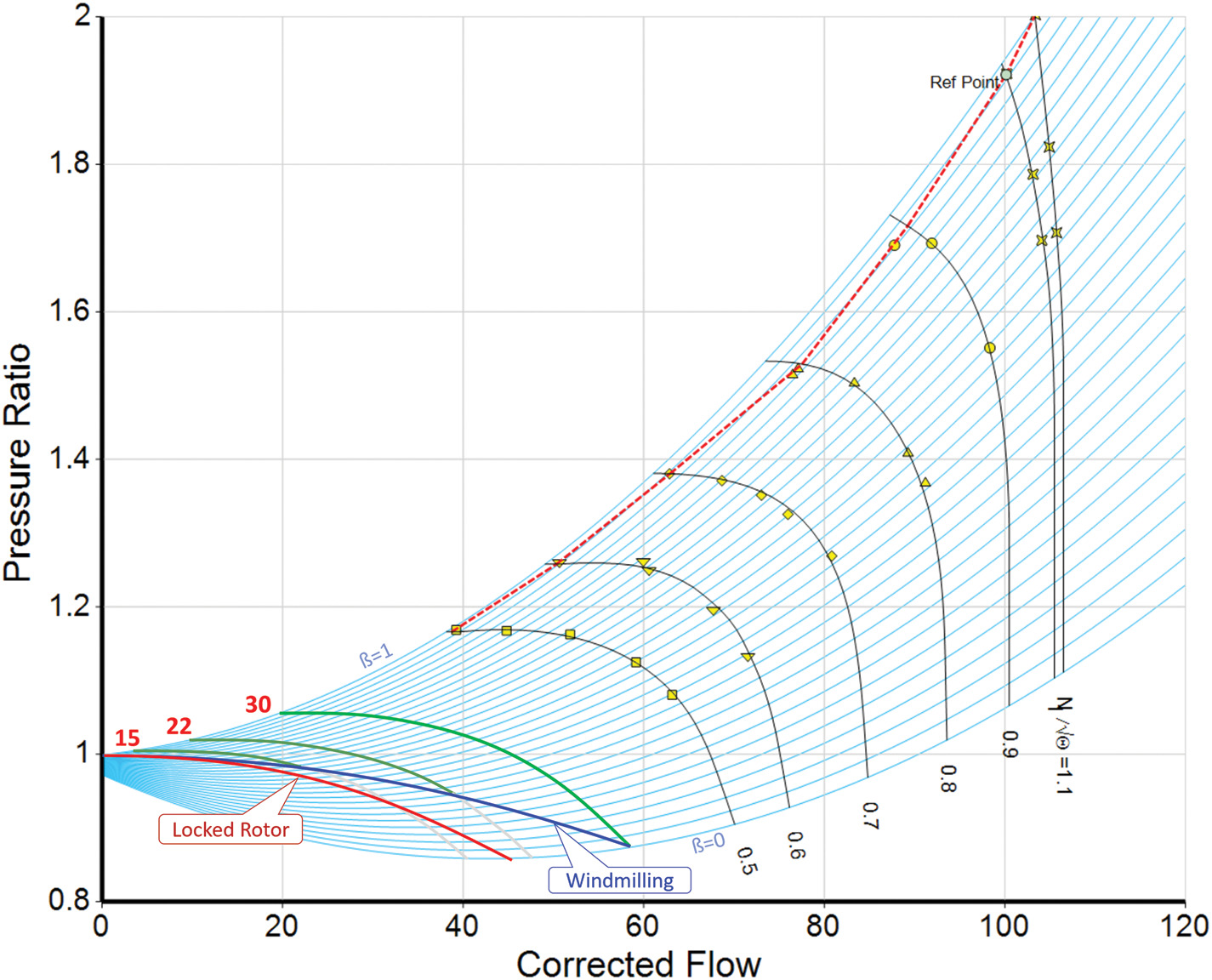
The accuracy problem at low speed can be reduced using the alternate definition of the β = 0 line shown in Figure 4. At the right end of the windmilling line all the data on a speed-line in the range from β = 0 to β = 1 are as meaningful as before. In the middle of the windmilling line, 22 out of 30 β-values make sense and at lower speeds, 15 β-values relate to useful data. The number of meaningful data points for a speed line still decreases with speed, but less so than before.
Creating data for sub-idle speeds with such a β-line grid is difficult, but there is a way around this problem: We split the β-line grid into two regions, one for the upper speed range and another one for the lower speed range. In the new low speed β-line grid we give the β-value a physical meaning: we define it as a line of constant ψ and Φ.
The two regions of the grid are connected at the grid dividing speed, which we select so that the torque/flow value at the high mass flow end is slightly less than zero. In the example of Figure 5, the grid dividing speed is chosen as 0.3; the low speed β-line grid describes the compressor performance in the grey region of Figure 6. In the plot, P2/P1 = f(W) all β-line parabolas begin at the origin {W = 0; P2/P1 = 1} with a slope of zero and end on the dividing speed line at the point which has the same β-value as the high-speed grid. In the low speed β-line grid all β-values between 0 and 1 are related through the physically meaningful properties ψ, ψis and Φ.
With the double set of parabolas, even the performance at relative speeds as low as 0.01 (1%) can be described accurately. The use of two sets of parabolas for compressor maps looks like an extraordinary idea but remember that the β-line grid used in the turbine performance maps of GasTurb also consists of two sets of parabolas corresponding to the lower and upper speed ranges.
Finding the shape of the β grid dividing speed line
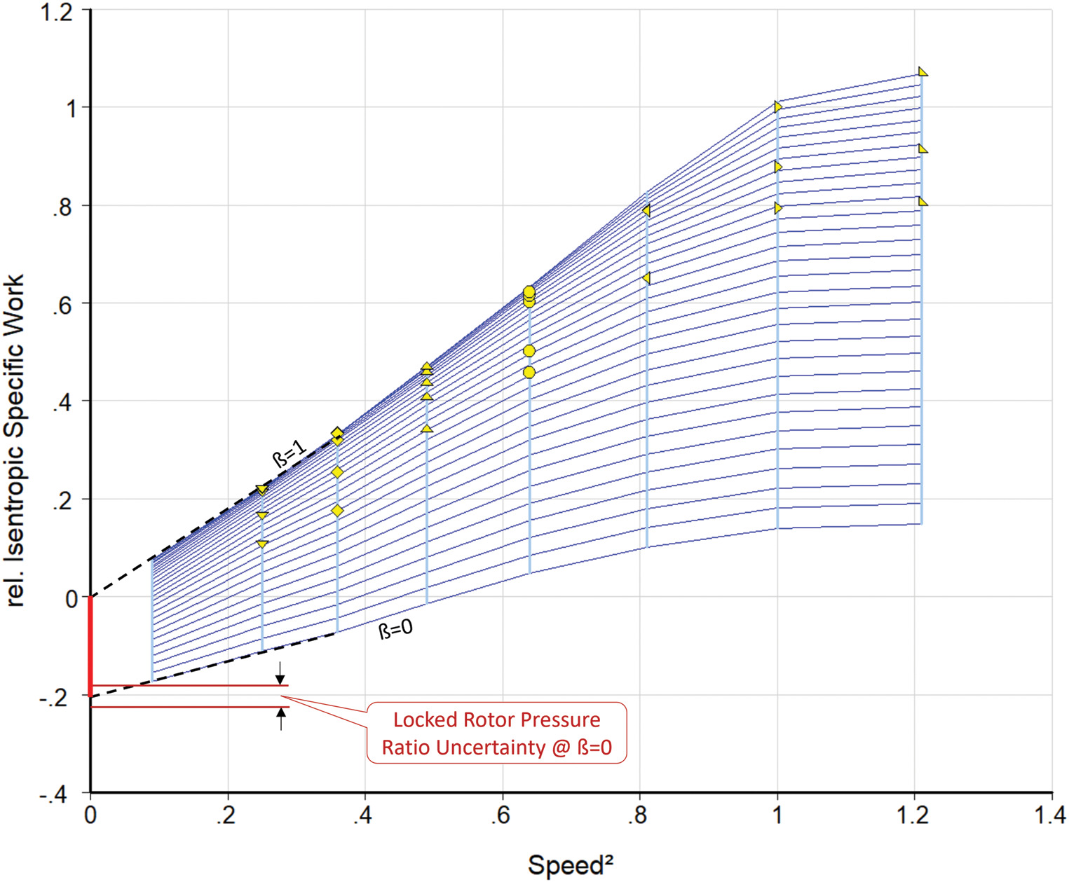
We chose 0.3 for the grid dividing speed because in the windmilling tests (Hatch, 1958) the highest spool speed was slightly less than 30%. We created this speed line by interpolation between the locked rotor line (speed = 0) and the lowest speed for which we have measured data. In our example this is N/√Θ = 0.5. To find the low mass flow point on the grid-dividing speed line N/√Θ = 0.3 we use a β-line grid in which the β = 1 parabola passes through the origin {W = 0; P2/P1 = 1}. Figure 7 shows that the isentropic specific work for β = 1 is nearly a straight line in the low-speed range when plotted over speed squared. Thus, linear interpolation of isentropic specific work His between zero (locked rotor) and (N/√Θ)2 = 0.25 is very well suited for finding the pressure ratio on the β = 1 line for any speed less than 0.5.
The remainder of the speed line N/√Θ = 0.3 is found by linear interpolation over speed squared along the other β-lines. The result depends on the assumed shape of the locked rotor parabola and on the position of the β = 0 line which together with the β = 1 line defines the β-line grid.
In Smooth C one can vary the assumed slope of the locked rotor parabola and observe what happens with the correlations between the many non-dimensional properties within the map. Figure 8 shows six views of the data for three different versions of the speed line N/√Θ = 0.3. The two dashed lines are interpolations between the locked rotor and N/√Θ = 0.5 for different values of the constant aN0 in Equation 6. The Ψ = f(Φ) and Trw/W = f(W) lines are both straight and parallel.

It cannot be expected that the application of the simple theory described above yields perfect alignment with the parameter correlations found in the known part of the map. The two dashed lines in the six pictures in Figure 8 should be considered as a guide for manually fine trimming the shape of the P2/P1 = f(W) and the Trq/W = f(W) lines in such a way that they fit best. Modifications applied in the middle part of the P2/P1 = f(W) correlation affect the shape of the efficiency correlation η = f(W) and the slope of the Trq/W = f(W) lines. Compressibility effects show up at the high mass flow end of the speed line. The blue lines in Figure 8 represent the best choice for the grid dividing speed line N/√Θ = 0.3 in the example map. It fits reasonably to the Ψis − Φ and Ψ − Φ correlations observed for the relative speeds 0.5, 0.6 and 0.7. The peak efficiency point is located on the straight line between the peak efficiency point on the N/√Θ = 0.5 line and zero in the plot Trq/W = f(W), as postulated by incompressible flow theory. The right ends of the blue lines bend downwards in the two middle pictures of Figure 8. This was introduced because the assumed boundary of the incompressible flow region is exceeded in that region.
Note that the manual adaptation of the final speed line to the known correlations makes the result independent of the choice of the β = 0 line. Engineering judgement affects the outcome, but the degree of freedom one has is not big when all the many correlations between the map parameters are considered thoroughly.
Completing the map
After having generated the grid dividing speed line, we can easily find the speed line for N/√Θ = 0.4 by interpolation between N/√Θ = 0.3 and 0.5. Adding lines for speeds less that the grid dividing value is especially easy because there the laws of incompressible flow are applicable. In the low-speed grid, the parabolic β-lines have a physical meaning: they are lines of constant Φ, Ψ and Ψis. Speed lines can be added in such a way that the curves Ψ = f(Φ) and Ψis = f(Φ) collapse. Manual corrections are applicable to the high mass flow end of the speed lines if compressibility corrections have been applied to the grid dividing speed line.
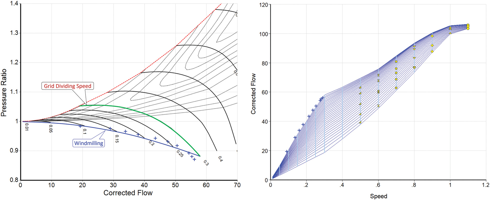
The left of Figure 9 shows the lower part of the extended map where the blue line (Ψ = 0) represents windmilling. The blue crosses are measured data – they line up reasonably well with the extended map. On the right the measured windmilling data are compared with the flow-speed correlation in the extended map.
Concluding remarks
Smooth C is criticized because its use requires some knowledge of compressor physics, and engineering judgement plays a role when creating a map from measured or calculated data. However, engineering judgement also plays a role when using other map extension methods.
Ferrer-Vidal’s (2018) sub-idle map generation method, for example, requires at least a preliminary mean-line geometry, which is used to calculate a torque-free characteristic and the locked rotor line. Interpolation between these two lines and the above-idle map is then carried out. Ferrer-Vidal admits that the calculated windmill signature (the ratio N/W) may need to be adjusted manually until the expected trend appears. This is also an example of the application of engineering judgement!
The use of analytical methods raises inevitable questions like: What is the origin of empirical constants and other input data needed for running the software? What are the limits of the applied methodology? Is it justifiable to apply it to exotic operating conditions like “locked rotor” or “windmilling”? User judgement always affects the outcome!
Turbofan starting simulations with a thermodynamic cycle program can begin at approximately 1% fan spool speed, see Kurzke (2023). Reasonable looking map extensions down to such low spool speeds can be created with the enhanced version of Smooth C and the use of this program to generate and extend compressor maps is by far less time consuming than any analytic method or the use of neural networks. The main advantage of Smooth C is that it offers many different views on the data simultaneously. Detection of inconsistencies and physically impossible characteristics is made easy and thus an engineer – with a basic knowledge of compressor physics – can generate high quality compressor maps. The significant difference of the enhanced Smooth C version when compared to previous versions of the program is that the β-line grid consists of low- and high-speed parts. In the low-speed part the β-lines have a physical meaning which justifies the application of incompressible flow theory.