
Introduction
A comprehensive literature survey of the simulation of engine starting has been published by Ferrand et al. (2018). Three model categories are identified, beginning with the so-called “torque” models which do not need component maps. Gas turbine parameters (mass flow, speed, pressures, temperatures etc.) are approximated by polynomials dependent on rotational speed, whose coefficients are determined by experiment. The second category of models uses a “black box” approach where physics is not considered. A large amount of training data is required to produce accurate results.
The third category are aero-thermodynamic models which use component maps. Anderson et al. (1997) describes in detail the challenges of such models with respect to windmilling simulations. Fuksman and Sirica (2011, 2012) discuss modelling techniques that ensure smooth operation, starting with engine off (zero speed) and continuing through the regions of starter engagement, fuel addition, and starter disengagement leading to normal engine operating regime. Bretschneider (2015) concentrates on modelling the crank phase of a ground start beginning with zero speed. He presents the physical effects happening during engine start and provides modelling solutions. Both Fuksman and Bretschneider apply their methodology to a separate flow high bypass turbofan while the remarks from Anderson et al. (1997) regard a wide range of different engine designs. A major challenge common to all aero-thermodynamic models is the acquisition of compressor and turbine maps with sub-idle regions.
As may be expected here, we discuss starting and windmilling simulations with a gas turbine performance program using extended compressor and turbine maps, generated with the methodologies described by Kurzke (2019) and (2020). The model illustrates a general understanding of what happens from when the starter is activated to when stabilized idle operation is reached. Operating lines in the compressor and turbine maps are predicted depending on starter torque, starter power, burner light-up and starter cut-off speed. The acceleration after burner light-up is controlled by a prescribed gas generator speed change per time
In the model the fuel flow to achieve the required acceleration is calculated, while in a real engine either the fuel flow or the exhaust gas temperature is scheduled, and the acceleration is a result. We deliberately do not use fuel flow as input because we want to develop an engine starting procedure which determines how the fuel flow should be scheduled.
Thermodynamic cycle model
In various parts of Kurzke and Halliwell (2018) it is shown that a physics-based performance program can reproduce measured data from an engine test bed quite well. There is no reason why the same approach cannot be used to address sub-idle operation; the laws of physics apply under all conditions. However, during starting and windmilling certain specific phenomena which are insignificant in the normal operating range between idle and full power must be considered. This applies equally to the behaviour of the modelling algorithms and the engine components.
The normal performance model for everyday use covers little more than the operation between idle and full power. Typically, the idle spool speed is around 30% for the low spool of turbofans and 60% for gas generators or single spool turbojets. Hence the first task in the simulation of starting is to extend the compressor and turbine maps to include sub-idle corrected speeds down to say 5–10% of the design value.
Compressors
Generating a map by calculation - including the sub-idle portion - is feasible, provided the geometry of the compressor is known in sufficient detail, but that is seldom the case. Apart from this, the agreement between measured data from a compressor rig test and the results of calculations is not always satisfactory - even in the range between idle and full power. Prediction of the surge line is especially problematic.
An alternative to the generation of a new map is to use one from a test of a similar compressor and scale it so it corresponds to the engine cycle under consideration. The problem with that approach is that compressor rig tests are usually limited to the speed range from idle to full load. The measured map needs to be extended to accommodate the engine starting and windmilling operating points.
A generally applicable map extension method must be able to generate maps which include regions where the pressure ratio is less than unity because such pressure ratios can occur during windmilling. Not all approaches to map extension found in the literature have that capability. Kurzke (2019) describes a physics-based compressor map extension method which does have that feature yet does not require geometry data to function.
In a cycle program to be used for starting and windmilling simulations, it is desirable to use the same set of compressor map data tables with corrected mass flow, pressure ratio and efficiency as functions of corrected speed and the auxiliary coordinate beta. However, there is a problem with respect to efficiency in the region near the pressure ratio of unity because there the efficiency jumps from −∞ to +∞, making interpolation impossible. Unfortunately, this is unavoidable when reading numbers from the map table during the performance calculation. However, the problem can easily be resolved by converting the efficiency table to one with corrected specific work ΔH/T.
That can be done either before loading the map into the cycle program or directly after loading the map tables from file. This approach has the advantage that any set of extended map tables can be used as it is, with no special map pre-processing for starting and windmilling simulations being required.
Note, that in the sub-idle region of any map, corrected specific work is a straight line when plotted against corrected flow. This makes reading interpolated values from the map table simple and accurate. Interpolation between tabulated speed values should be linear against speed squared. This corresponds with constant aerodynamic loading which is defined as specific work over speed squared.
Turbines
In a map of a gas generator turbine all operating points between idle and full power are close to the cycle design point. The quality of the gas generator turbine map is of secondary importance for accuracy of the simulation between idle and full power. The turbine map needs to be known only over a small region of corrected speeds and pressure ratios.
In contrast, engine starting simulations cover much more of the map because the operating point moves from zero-mass flow and unity pressure ratio to the full power region. High quality of the turbine performance representation is critical for starting simulations. In the low-speed part of a turbine map there are big efficiency changes over a small pressure ratio range. The use of beta lines (auxiliary coordinates) with narrow spacing at low corrected spool speeds is especially suited for this purpose.
In an LPT map, the operating lines from full power down to idle are generally longer than those in a gas generator turbine equivalent. In general, a much bigger region needs to be covered, so the usual range of the corresponding tables is insufficient to simulate engine starting. The map regions from zero to idle corrected speed as well where pressure ratio falls below one (where windmilling occurs) are missing – so the map must be extended.
Calculating a turbine map, including the sub-idle and windmilling regions, is feasible, provided the geometry of the blades and vanes is known in sufficient detail. Unfortunately, the required information is inaccessible in many cases. We have the same situation as for compressors and need to extend the maps we would normally use to quantify the performance range between idle and full power. Kurzke (2020) describes the theory of a new turbine map extension method and gives practical advice.
Combustor
Any steady state operating point needs a certain amount of energy, which is provided by burning fuel. For normal operations of modern engines, the burning process is close to perfect, but for starting it is far from this and we get significantly less heat from a given amount of fuel than is possible theoretically.
Yes, it is difficult to predict combustion efficiency during engine start. However, do we really need accurate ηcomb values for a useful simulation of ground and altitude starting? What are the implications if we use an inaccurate combustor model? Combustion efficiency affects the amount of fuel needed for heating up the air from burner inlet temperature T3 to the turbine inlet temperature T4.
The fuel mass flow is generally small compared to the air mass flow. At full load the fuel-air-ratio ranges from 0.025 to 0.035, while at idle it is around 0.01. Thus, changes in combustion efficiency demand changes in only about 1% of the total gas mass flow. Having an uncertainty of up to ±30% in combustion efficiency is not a big issue.
Mixer
Mach numbers in the mixer of a turbofan are low during engine start and windmilling. Therefore, we can simplify the complex iterative algorithm which is applied in the normal engine operating range. Ignoring Mach number effects enables the use of equations which can be solved directly. That makes the overall cycle model more robust, especially at the beginning of a start simulation.
Starter
We can describe the performance characteristics of the starter with three numbers: maximum torque, torque slope over spool speed and power. The torque increases to its maximum value within the first seconds of the starting simulation and continues at this level with the given slope = f(N) until the starter power limit is reached. Torque drops to zero within seconds after the starter cut-off speed is reached.
Rotor inertia
It is not possible to calculate starting times without values for rotor inertias. If no better values are available, you may use the results from a conceptual engine design program like that described by Kurzke and Halliwell (2018).
Steady state off-design algorithm
The same reference summarizes the mathematics needed as a foundation for the synthesis of steady state off-design operating points in the normal operating range between idle and full power. When a gas generator spool speed NGG is specified, the Newton Raphson algorithm will find a solution which satisfies the mass flow continuity between components, power balances for each spool, mass flow restrictions for nozzles and pressure balances in mixers.
This algorithm also works in the sub-idle range of the model, but convergence problems are likely to occur as spool speeds decrease. Nevertheless, one can run a two-spool mixed flow turbofan model at sea level static conditions down to less than 2% gas generator speed provided the compressor and turbine maps are physically sound and successive operating points do not differ too much in NGG.
In a Newton-Raphson iteration there are variables and errors, and the algorithm manipulates the variables in such a way that, finally, the errors are less than epsilon. Among other things, the reliability of the process depends on how the iteration errors are calculated. Let us examine the iteration error which evaluates discrepancies in mass flow between an upstream component and the flow capacity of a turbine. Usually, the HP turbine flow error is defined as
This definition of iteration error becomes problematic at exceptionally low sub-idle speeds, when the term W41Rmap becomes small. This makes the iteration error overly sensitive to a slight change in the iteration variables. The algorithm is made more robust by replacing this term in the denominator with the design value to give the following equation:
One can calculate steady state off-design operating points for very low spool speeds, and since we have explained above why the results of such calculations are essentially independent of combustion efficiency, we know the locations of all turbomachinery operating points in their respective maps are unaffected by the performance of the burner.
The ability to calculate steady state points down to extremely low gas generator speeds has two supplementary benefits. It provides a check on whether the compressor and turbine map extensions to low speeds make sense, and it creates a starting point to establish a stable operating point with zero fuel flow in crank mode.
Pick a point at say 20% gas generator speed from the steady state operating line and do a parametric study with power offtake PWX, beginning with zero and decreasing in steps. The fuel flow needed for running the engine with 20% NGG will decrease sequentially till it approaches zero. The prevailing (negative) power offtake corresponds to the shaft power needed for cranking the engine at that speed.
A similar procedure yields a stable windmilling point: Begin with static conditions and zero power offtake, keep the gas generator speed constant, and increase the flight Mach number in steps. Again, the fuel flow will decrease sequentially till it is zero. This yields the windmilling Mach number at which the gas generator speed is 20%.
There are special cycle calculation modes for cranking and windmilling. In the “Cranking” mode the usual iteration variable T4 is replaced by power offtake PWX and in the “Windmilling” mode T4 is replaced by flight Mach number. Fuel flow is zero in both sets of calculations.
Engine control in transient operation
Normal operating range
In the operating range of a real fixed geometry engine between idle and full power, changing the fuel flow is the only way to influence the power. In a real engine, sensors deliver signals to the control system which compares the power delivered with the power demanded. The fuel flow is either increased or decreased according to the differences between current and demanded value. In a simulation, however, it is better to control fuel flow indirectly via fuel-air-ratio because this is much less dependent on ambient conditions. Absolute fuel flow varies with engine inlet total pressure and temperature as well as spool speed, but the fuel-air-ratio is pretty much constant.
The operation of the PID controller in an engine model may be governed by setting selected combinations of the constants CP (Proportional Control Constant), CI (Integral Control Constant) and CD (Differential Control Constant). Note that the numerical values for these control constants depend on the simulation algorithm: When fuel flow is the iteration variable, the control constants need to be adapted as engine inlet total pressure and temperature change because fuel mass flow is not a non-dimensional quantity. When fuel-air-ratio is the iteration variable, however, the control constants remain valid for a wide range of P2 and T2.
Engine starting
Engine starting is a special transient event in which three different calculation modes are combined, depending on the prevailing energy source. At the beginning the starter is the sole energy source and there is no fuel flow. The algorithm is like that used in crank mode. After combustor light-up, there are two energy sources: the fuel and the starter. Finally, after starter cut-off speed is reached, only the fuel supplies energy.
Starting a mixed flow turbofan
For the following example we use a low bypass ratio turbofan with the following main parameters:
| Thrust | 35 kN | Bypass Ratio | 0.5 | Mass Flow | 50 kg/s |
| T4 | 1,600 K | P3/P2 | 20.79 | LPC P21/P2 | 3 |
| HPC P3/P25 | 7 | LP Inertia | 4.12 kg m2 | HP Inertia | 2.1 kg m2 |
Ideally, a ground starting simulation begins with zero speed and zero mass flow. All pressure ratios are unity, all temperatures and pressures are equal to ambient values. This unique operating point is trivial but impossible to calculate with the normal thermodynamic cycle model, for numerical reasons. If we want to use our standard cycle calculation program, we cannot begin with zero speed. We need results for an operating point at exceptionally low spool speed, from which we can initiate a starting simulation. That will be our operating point at time zero of the simulation.
Preparing the start simulation
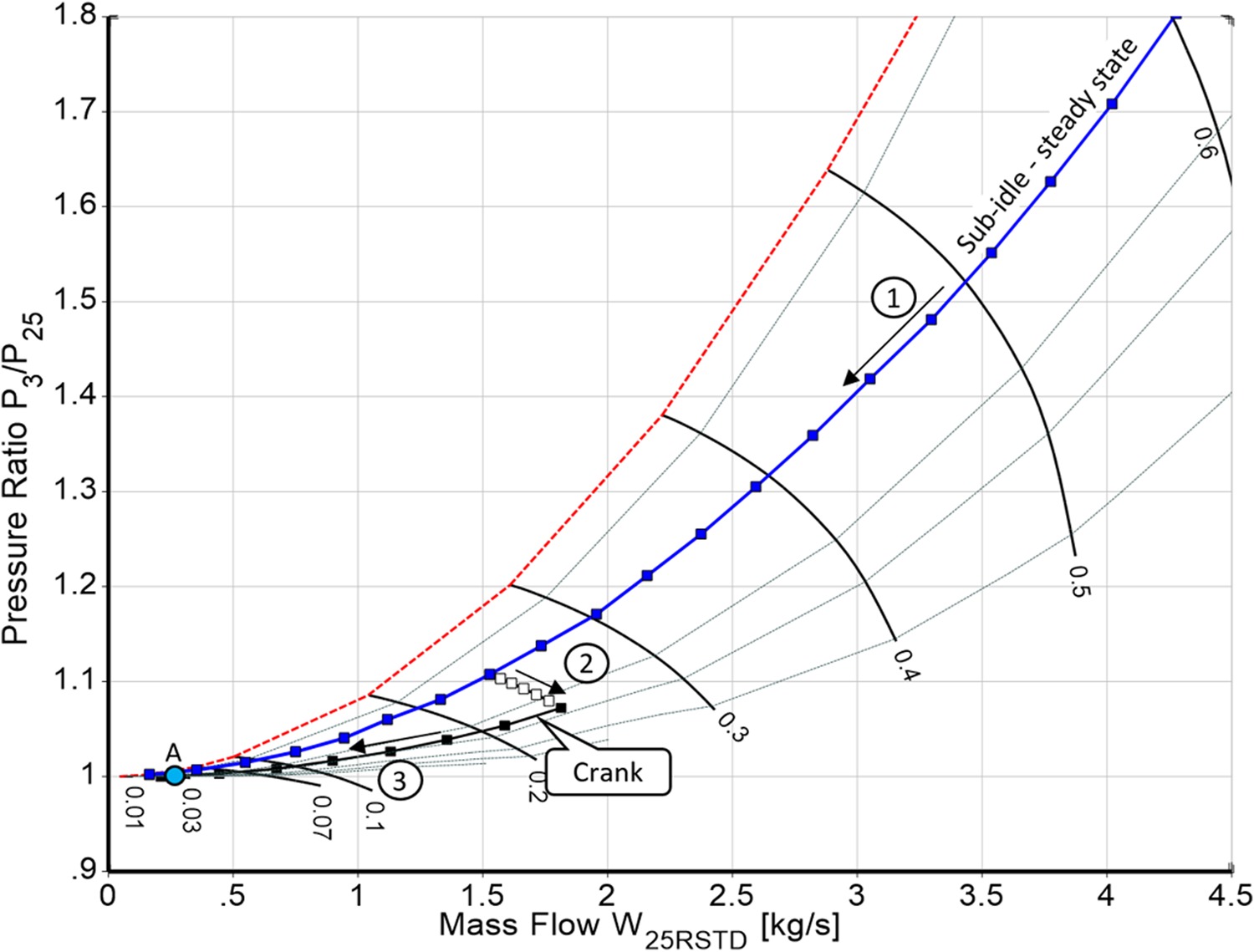
The extended compressor and turbine maps are fully consistent with the normal performance model. To find an operating point suitable for beginning an engine starting simulation, the first preparatory step (1) is to run an operating line with downward steps of gas generator spool speed until the calculation fails to converge.
An important lesson from running the steady state performance simulation is the robustness of the model. The lower the achievable gas generator speed the better. Problems are likely to be encountered during engine starting. For example, the operating line in the gas generator compressor map might be too near to the surge line or even beyond it. A bleed valve downstream of the compressor then needs to be opened during engine starting to alleviate such a problem.
In the second preparatory step (2), we search for a steady state operating point with energy from a starter rather than from fuel. In other words, we look for a crank point. In our steady state performance model, we replace the energy provided by the fuel with shaft power from a starter and do a parametric study at a given gas generator spool speed of say 20% in which the amount of negative power off-take decreases in steps, i.e., power is being inserted. The fuel flow decreases sequentially until it is near zero. Now we have good estimates of the iteration variables suitable for finding a true crank point with exactly zero fuel flow.
The third step of the engine start simulation preparation (3) is the calculation of an operating line in the cranking mode down to low gas generator speed. Using a small NGG step-size is crucial for reaching extremely low gas generator spool speeds.
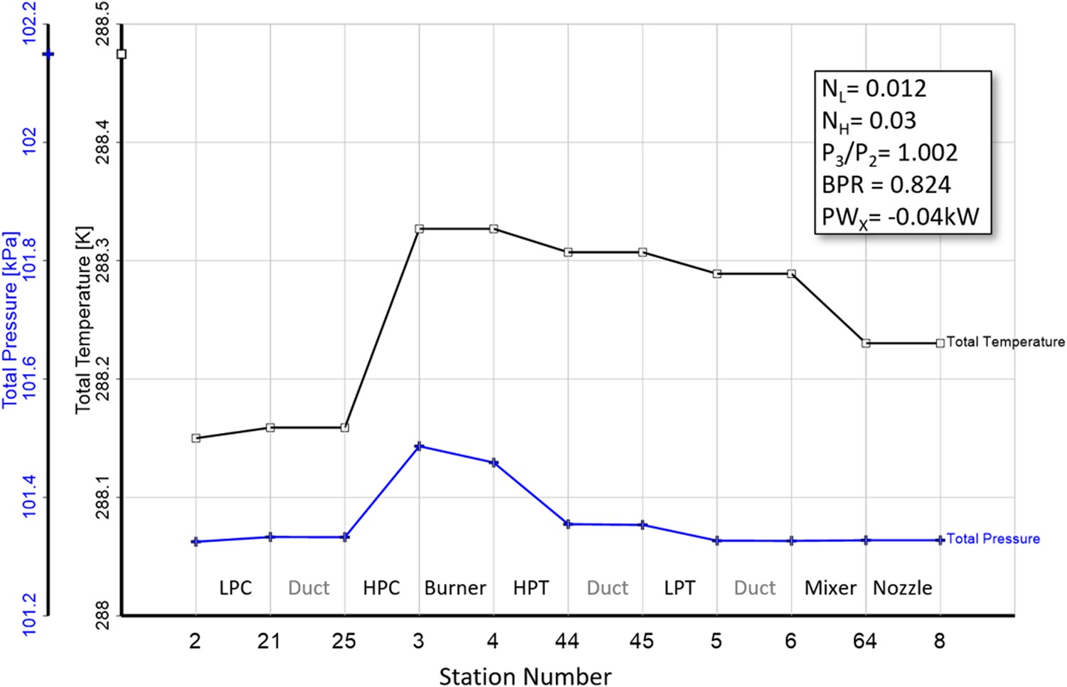
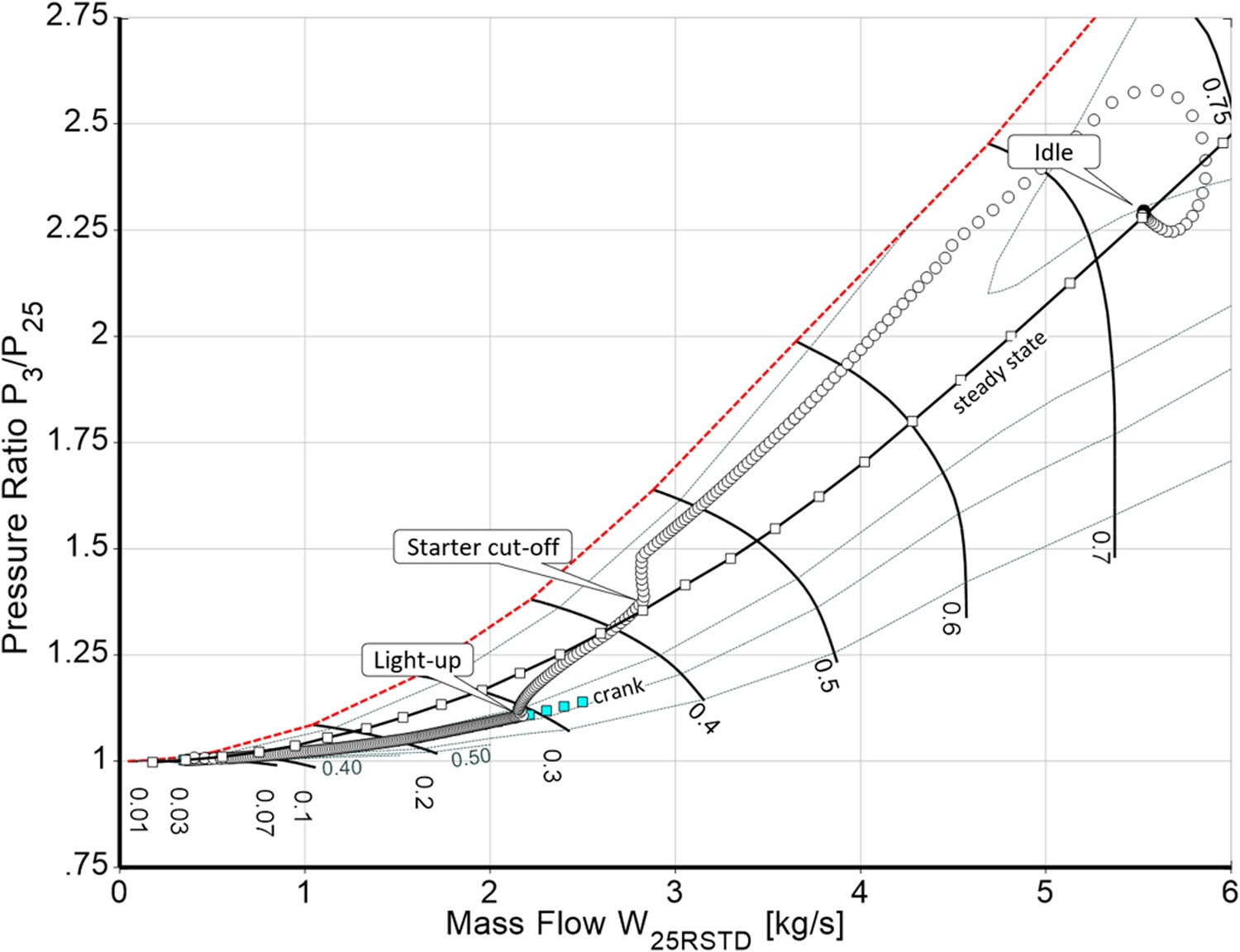
Figure 1 explains the three preparatory steps for the engine start simulation (which will begin with point A) in the HPC map and Figure 2 shows how total temperature and pressure vary from engine entry to exit.
Sequence of events
Figure 3 shows an overview of the engine start simulation. It begins with point A which is a steady state crank point with the relative speeds of NL = 0.012 and NH = 0.03. The starter is the only energy source until the light-up speed is reached. From that moment the burning fuel contributes additional energy to the cycle. The transient PID controller determines how much fuel is delivered to the combustor. The demanded spool speed is the gas generator idle speed, which is much higher than the burner light-up speed. The proportional controller tries to increase the fuel flow quickly to close the gap between the prevailing speed and that at idle. This moves the operating point in the gas generator compressor map towards the surge line. To prevent surge, we need to restrict the fuel flow, and this can be done by limiting either the fuel-air-ratio or the acceleration
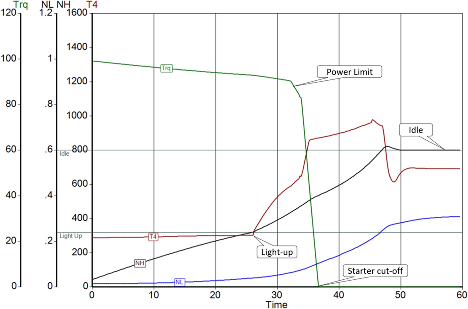
A special phenomenon can occur while starting a low bypass ratio mixed flow turbofan: flow reversal occurs in the bypass duct. As can be seen in Figure 3, in the first 25 s, during cranking, the HP-spool accelerates much faster than the LP-spool. The gas generator captures more and more of the air delivered by the fan and the bypass ratio decreases until all the fan air is ingested by the engine core.
From that moment on, the fan can no longer deliver all the air demanded by the core compressor and additional air is drawn from the exit of the core, passing through the bypass channel in the reverse direction.
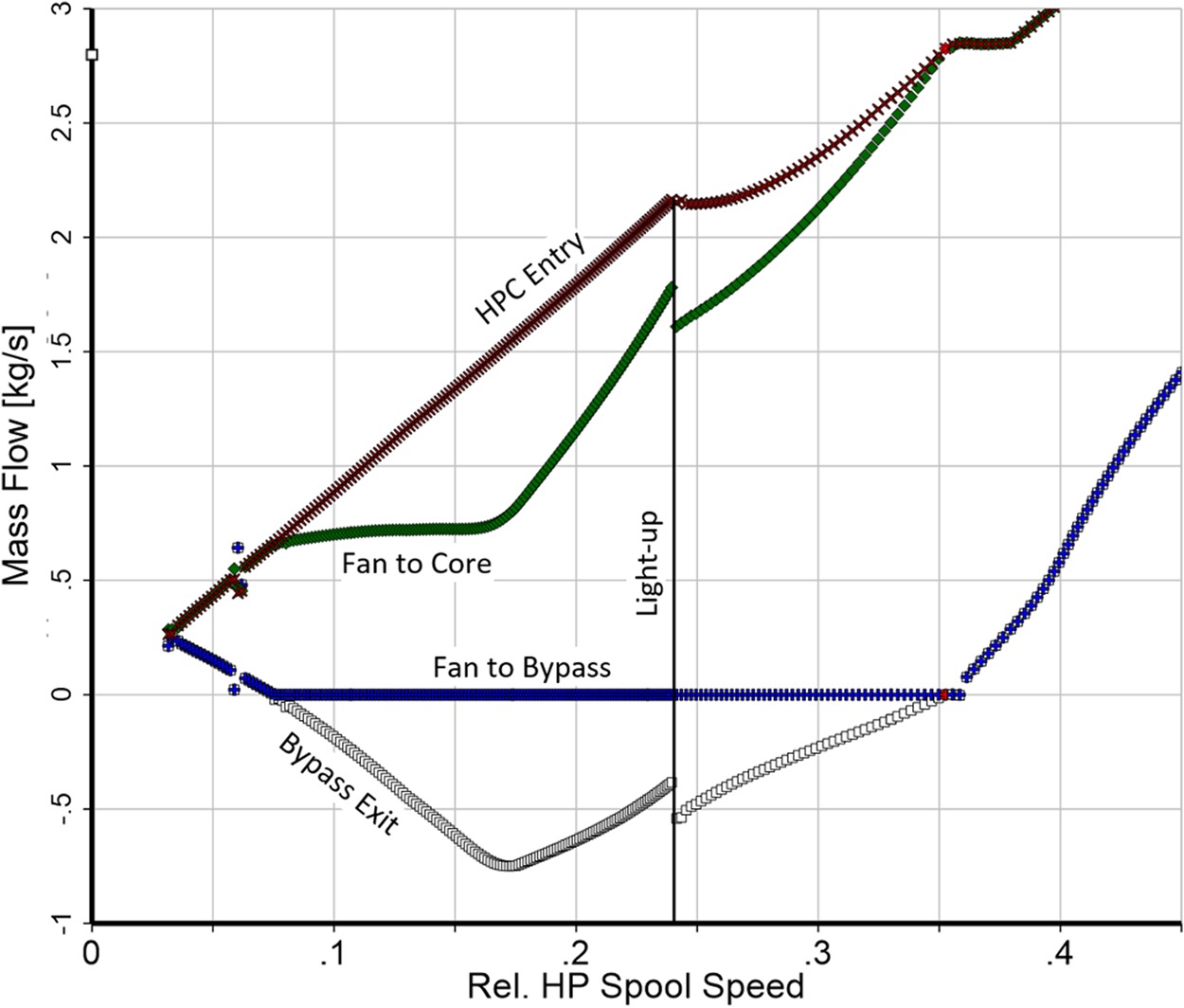
Figure 4 shows the various mass flows as functions of relative HP spool speed. In the first phase of the transient simulation, the fan delivers less air than that during steady state since its speed lags the core speed. After the relative gas generator speed has reached 0.075 all the fan inlet flow goes to the core and nothing to the bypass. The situation changes after burner light-up, when the HP compressor operating line moves away from the steady state operating line. Flow reversal in the bypass duct ends when NH passes 0.35.
Numerical issues
It is desirable to begin the simulation of engine starting at the lowest gas generator speed for which the crank calculation converges. Keep in mind, however, that the numerical solution at extremely low spool speeds might be inaccurate due to unavoidable numerical noise which is magnified the closer the component pressure ratios come to one. Gas generator speeds less than 2% of the design value - usually accompanied by low pressure spool speeds of around 1% - are suitable as starting points only if physically sound compressor and turbine maps are available. Such maps must include data for relative corrected spool speeds from 0.01 upwards.
The calculation does not need to stop if it fails to converge at zero time. Simply begin the next time step with the iteration variable set at the value which created the smallest iteration errors for time zero. If you are lucky, you will then get a converged solution for the first timestep. If not, continue with a best guess at a value of the iteration variable for the next timestep. It can take up to ten timesteps for the Newton Raphson iteration to converge for the first time. Store this solution and use it as a guess for the time zero case the next time you begin with the simulation of the engine start. If no converged solution is found for the first 10 timesteps, try again with a different timestep or starter torque.
Figure 5 shows the full engine starting process in the HP compressor map.
Windmilling of a turbofan
At an airport, on a windy day, one can see parked aircraft with rotating fans. This is due to the total pressure at the engine face being slightly higher than the static pressure around the exhaust. There is a sort of ram pressure ratio which corresponds to an exceptionally low flight Mach number. The fans rotate faster during flight when an engine is shut down because then the ram pressure ratio is bigger. The reverse may also happen when an aircraft is parked in a tailwind and the fan is seen to rotate in the opposite direction.
Some questions of interest in the context of windmilling are:
How much power can be taken from the engine?
What is the drag of a shut-down engine?
How big is the air mass flow?
What is the burner inlet condition for a re-light attempt?
Algorithm
In off-design simulations, one frequently selects the operating state of the engine by specifying the gas generator spool speed. The amount of fuel required for attaining this speed is found by iteration. In the simulation of cranking the engine at a certain spool speed, the required starter power is found by iteration. The windmilling simulation can be set up in a similar manner by specifying the gas generator spool speed and iterating to the correct the ram ratio P2/Pamb, via the flight Mach number.
The three off-design algorithms differ in only one of the iteration variables employed in the Newton-Raphson iteration:
In normal flight when fuel is the energy provider, T4 is the iteration variable.
In cranking, starter power is the iteration variable.
In windmilling, the flight Mach number is the iteration variable.
We saw that the calculation of the steady state cranking point only works well at spool speeds above one to two percent of the design value, while a windmilling simulation is compromised if the flight Mach number is extremely low. Therefore, it follows that the calculation of a series of windmilling points should begin at high flight speed with the Mach number being reduced in small steps. Numerical problems will determine the low-speed limit.
The operating points in the compressor and turbine maps during windmilling are remote from the normal steady state operating line. The Newton-Raphson iteration often fails to converge when switching the calculation mode directly from normal to windmilling. We can solve this problem by approaching the windmilling operating point in small steps, beginning with a converged steady state operating point. First, run a steady state operating line for static conditions (Mach number zero) down to low gas generator spool speeds. Then pick the point with a relative gas generator spool speed of NGG = 0.2, for example, and use it to initiate a parametric study with increasing flight Mach number. The energy from combustion decreases with increasing ram pressure ratio until finally the calculated fuel flow approaches zero and a suitable starting point for the windmilling algorithm is reached. The windmilling calculation employs flight Mach number as an iteration variable instead of T4 and sets the fuel flow to zero.
Results
Let’s examine the behaviour of a geared turbofan model during windmilling using the following main characteristics for ISA SLS:
| Thrust | 205 kN | Bypass Ratio | 12 | Mass Flow | 814 kg/s |
| T4 | 1,850 K | P3/P2 | 45 | LPC P21/P2 | 1.43 |
| IPC P24/P22 | 2.45 | HPC P3/P25 | 15 |
The calculation sequence is the same as described above. We begin by running a steady state operating line for static conditions down to low spool speed. From the results, we pick the point at relative gas generator speed 0.2 as the basis for a parametric study with increasing flight Mach number. From these results, we select the point with the lowest fuel flow and switch to the windmilling calculation mode.
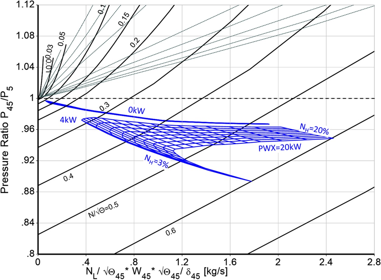
The solution for the windmilling cycle calculation is presented in Figure 6. The flight Mach number of 0.403 was found by iteration. Note that the relative fan speed of 0.253 is significantly higher than the gas generator speed, the fan pressure ratios is less than unity and the total temperature is increasing in the LPT. That means the fan generates power and the LPT consumes power – the opposite of normal engine behaviour!

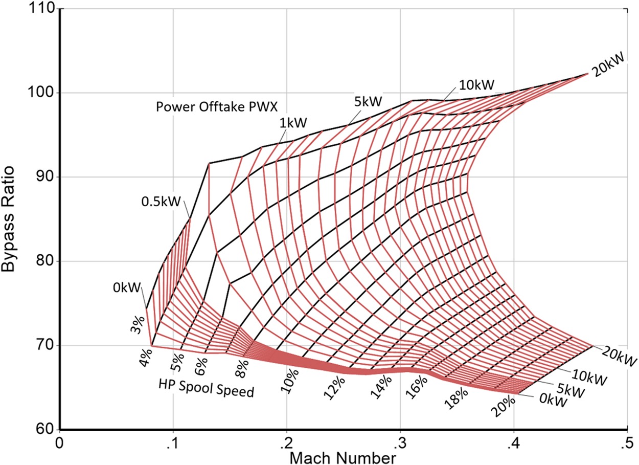
Next, we run a parametric study in the windmilling mode with gas generator spool speed and power-offtake PWX as parameters. Figure 7 shows how high the bypass ratio can become during windmilling. At a 20% gas generator speed the mass flow through the bypass duct is 64 times of that entering the core! The lower the gas generator speed, the more pronounced is the influence of flight Mach number on the amount of power offtake.
The fan behaves like a true windmill - it generates power. The operating line in the fan map of Figure 8 is controlled by the bypass nozzle area - the power taken from the gas generator spool does not affect it. The booster operability is a problem – even with a bleed valve downstream are the calculated operating points beyond the estimated surge line (Figure 9).


The last component considered is the LPT. This turbine acts like a compressor and consumes the energy provided by the windmilling fan. Note that for the calculation of LPT operating points we need a map which covers pressure ratios less than one, as shown in Figure 10.
Finally, let us have a look at the drag which the windmilling engine causes. All operating points collapse onto a single line of negative net thrust FN = f(Mach). Higher PWX requires higher Mach number, and this corresponds to more drag, see Figure 11.
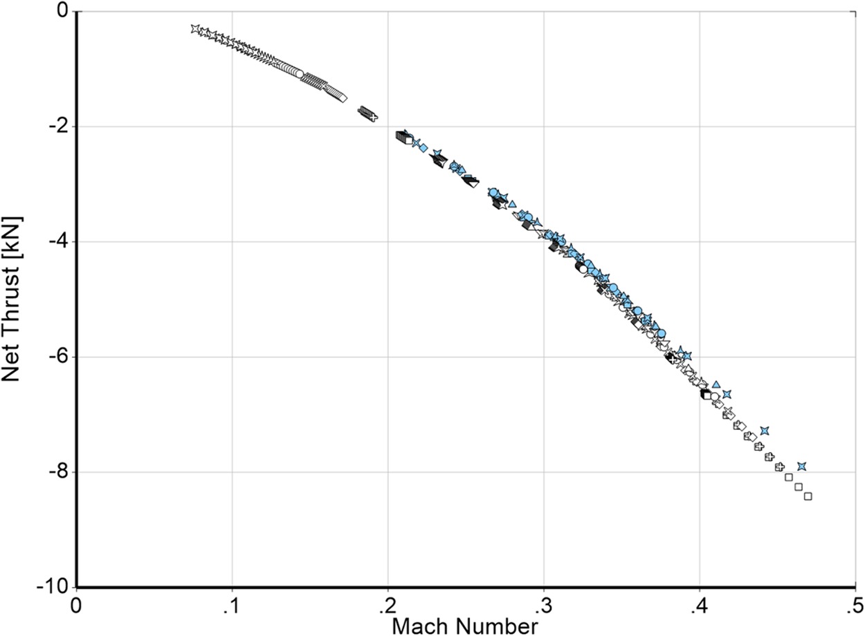
Note that the calculated relationship between thrust and Mach number is only part of the story. The nacelle is designed to capture a high corrected flow W2Rstd (more than 800 kg/s at high rotational speeds), but during windmilling, especially at low flight Mach numbers, less than one third of this flow is swallowed by the fan. The excess air creates spillage drag which must additionally be accounted for in the true (negative) net thrust.
Conclusions
This paper confirms that the map extension methodologies published by the author in 2019 and 2020 produce reasonable maps. In the mixed flow turbofan example two compressor and two turbine maps are combined in the cycle calculation and in the turbofan windmilling example even five maps are used. Other applications of the same cycle calculation program deal with starting and windmilling of single and two-spool turbojets as well as a two-spool turboshaft. In total five different compressor maps and three turbine maps have been extended and applied in starting and windmilling simulations.
Simulating engine starting and windmilling is not a magical art. The laws of physics still apply at these somewhat exotic operating conditions. The model predicts combustor entry pressure, temperature and mass flow for ground starting and in-flight relight. These may be used by combustion specialists to predict combustion efficiency or specify a combustor rig test. More detailed models contain engine-specific combustion efficiency models and ignition limits as well as accounting for combustor lean and rich blow-out, for example.
For altitude relight studies, detailed models of the external gearbox drag and the bearing losses - both of which depend on oil viscosity and are therefore functions of oil temperature - are needed. Parasitic losses of engine-driven accessories take a higher percentage of the HP turbine power at high altitude. This reduces the gas generator windmilling speed and can even stop the rotor at low flight Mach number. Deviations of the modelling results from full engine test data are expected due to these and other associated uncertainties. Combustor light-up and combustion efficiency immediately after ignition are random effects to some degree and that makes absolute agreement between model and reality improbable.