

Introduction
A critical challenge impeding the advancement of hypersonic propulsion systems lies in the pronounced thermal extremes encountered during operation (Kays and London, 1984; Murray et al., 2001; Sato et al., 2003; Kobayashi, 2004; Varvill, 2010; Hempsell, 2011, 2013; Feast, 2020; Meng et al., 2021; Zou et al., 2022). At Mach numbers exceeding 3, the stagnation temperature of the engine inlet flow reaches 600 K, exhibiting an exponential growth pattern with increasing Mach number. When the Mach number surpasses 5, the compressor inlet temperature exceeds 1,300 K, a condition incompatible with existing compressor designs. Consequently, effective thermal management strategies—either through heat dissipation or utilization—must be implemented. To address propulsion requirements at high Mach numbers, researchers have proposed novel engine concepts such as scramjets, pulse detonation engines (PDEs), rotating detonation engines (RDEs), and oblique detonation engines (ODEs). These systems eliminate multistage turbomachinery by leveraging the kinetic energy of hypersonic inflow and its thermal conversion to sustain operation. However, these propulsion methods face inherent limitations, including ignition difficulties and limited self-sustaining operational durations.
Subsequent developments introduced combined-cycle propulsion systems (Dong, 2018), wherein conventional engines are integrated with advanced thermodynamic cycles to mitigate startup challenges. Nevertheless, a new issue arises: both conventional and novel propulsion systems exhibit suboptimal performance in the Mach 3–5 regime, characterized by significant thrust degradation. This underscores that mere mechanical integration without corresponding thermodynamic cycle optimization remains insufficient to overcome the “thrust gap” phenomenon. Subsequent research efforts have led to the proposal of adaptive thermodynamic cycle systems and precooled engine concepts. The former adopts a dual-flowpath configuration inspired by the SR-71 Blackbird's propulsion system, enabling the activation of distinct flow-paths across varying Mach numbers to switch between multiple operational modes (three or more). This approach integrates thermodynamic cycles with structural design, significantly increasing system complexity in terms of both mechanical architecture and control logic. However, it effectively mitigates the limitations inherent in conventional combined-cycle propulsion systems that rely on simplistic mode transitions (Dong, 2018).
The precooled engine, as an alternative solution, innovatively incorporates the thermodynamic principles of intercooled-recuperated engines while further amplifying their energy recovery advantages. By integrating a precooler into the intake system to absorb stagnation heat from incoming air—later released in the combustion chamber or afterburner—this design achieves superior specific impulse, thereby overcoming the aforementioned propulsion challenges (Lee, 2017; Zou et al., 2022). The precooler serves as the core component of this system. Compared to industrial heat exchangers, it demands exceptional performance metrics: ultrahigh heat transfer density, compact structural packaging, minimal flow resistance, and lightweight construction. These requirements impose elevated standards for design, experimental validation, and manufacturing processes (Chen et al., 2019, 2022; Li et al., 2022, 2023; He and Li, 2024; Xu et al., 2024). Furthermore, the coupling of strongly variable material properties with extreme thermal environments results in complex fluid-thermal interaction mechanisms, introducing substantial uncertainties in precooler performance prediction. Such complexities establish more stringent conditions for the practical implementation of precooling technology in aerospace propulsion systems. First, traditional precooler design methods have been discussed to some extent in Reference (Li et al., 2022) of this paper. Based on this, the author identifies two main limitations: (1) Applicability of empirical correlations for convective heat transfer (this paper does not delve further into this aspect). (2) The level of refinement in the design method and its ability to capture real-world conditions. The characteristics of the supersonic thermal environment include extremely high heat flux density and high stagnation Mach number at the inlet (representing the gas side in this study). These factors lead to design requirements such as low flow resistance in the heat exchanger, Consequently, a low Reynolds number on the gas side. These constraints and features exceed the applicability boundaries of previous studies to some extent, necessitating experimental supplementation and validation. Currently, low-dimensional model predictions lack sufficient refinement and often fail to account for issues such as non-uniform parameter distribution encountered in real-world applications. Additionally, periodic models are frequently employed, leading to oversimplification (“generalizing from a partial perspective”). Therefore, experimental data are required to correct empirical correlations and support insufficiently refined models for accurate performance prediction.
This study investigates a typical precooler with fixed geometric configuration, employing supercritical carbon dioxide (sCO2) as the working fluid—a well-established medium in current thermal management research (Ma, 2016; Li and Yu, 2021; Moradkhani et al., 2023). The experimental phase initially characterized the precooler's hydrodynamic and thermal performance through systematic measurements, yielding comprehensive flow resistance and heat transfer coefficient curves. Building upon these empirical results, the analysis establishes intrinsic connections between precooler design methodology and performance evaluation criteria. The study identifies two critical parameters governing the assessment (and design) framework: internal flow resistance and external convective heat transfer coefficients. Subsequent methodology development proceeds through three analytical stages: Firstly, derivation of an empirical correlation between internal core-region friction factors and Reynolds numbers, followed by isolation and formulation of external flow heat transfer coefficient correlations with Reynolds number. Finally, iterative refinement based on the Kays & London loss model (Kays and London, 1984) of these empirical relationships through experimental data regression, followed by validation against independent test results. The finalized correlations demonstrate satisfactory agreement with experimental measurements, providing an enhanced engineering design tool for precooler development.
Geometric model
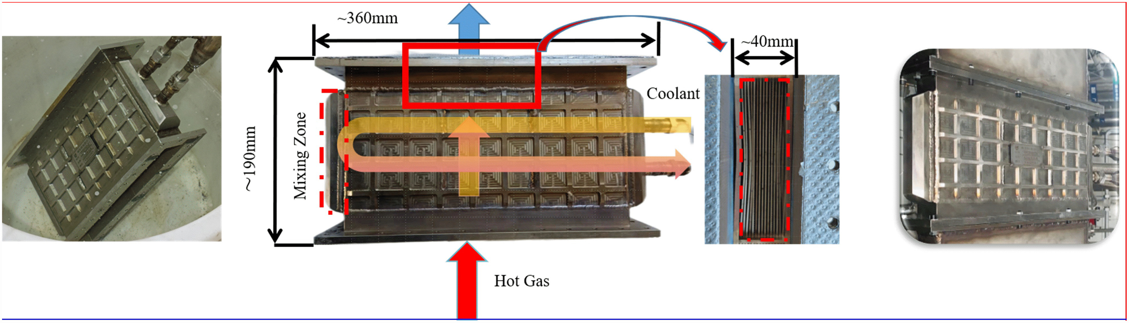
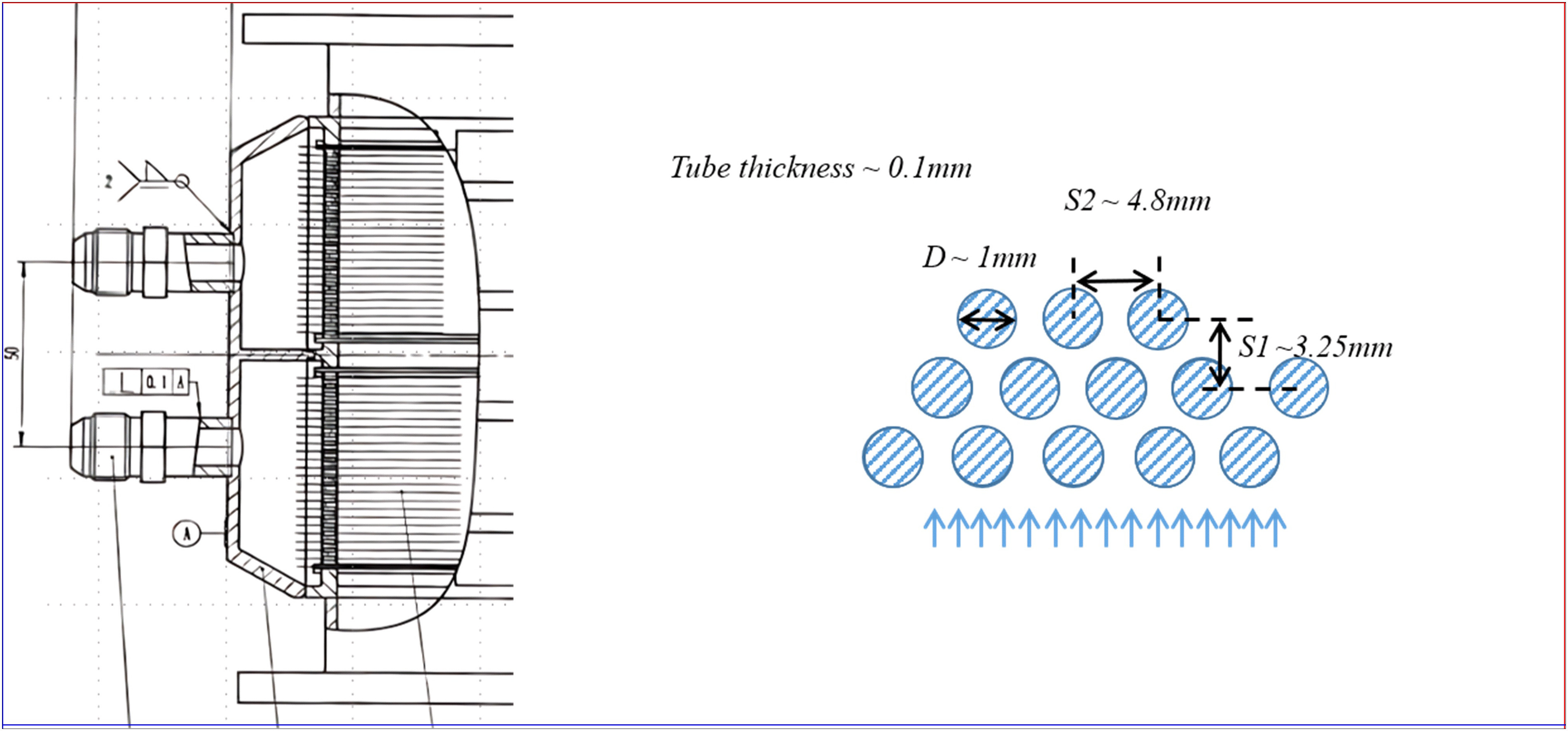
The precooler model employed in this study is illustrated in Figure 1, with detailed geometric parameters provided in Table 1. Figure 2 presents a cross-sectional view of the precooler header and tube bundle, indicating a cross-flow arrangement with one side mixed and the other side unmixed.
Introduction to the experimental validation system and test conditions
A detailed description of the experimental system can be found in Reference (Chen et al., 2022). Here, this paper primarily focus on the test conditions. In this study, the experimental conditions are divided into two groups, each consisting of 15 cases. The first group of conditions Table 2 is designed to obtain the corrected empirical correlations for flow resistance and heat transfer, while the second group Table 3 serves as validation cases, primarily used to verify whether the evaluation model under the current design framework can provide reasonably accurate assessment results. This study employs supercritical CO2 as the working fluid. As shown in Table 2, the inlet pressure and temperature significantly exceed the critical point (7.3 MPa and 305 K), meaning all operating conditions remain entirely within the supercritical state.
Table 2.
Inverse design data in experiment.
Table 3.
Validation condition data in experiment.
Analysis of flow and heat transfer characteristics in the SCO2 precooler
Heat transfer capacity and thermal balance deviation of the heat exchanger
As shown in Figure 3, the heat transfer capacity during the experiment varies with the mass flow ratio of CO2/air, while the air-side temperature is maintained within 800 ± 40 K. When the air flow rate increases, the heat transfer capacity also rises at the same mass flow ratio (evidenced by the parallel vertical trend lines). Overall, the heat transfer capacity exhibits an approximately linear growth trend with increasing CO2 flow rate.
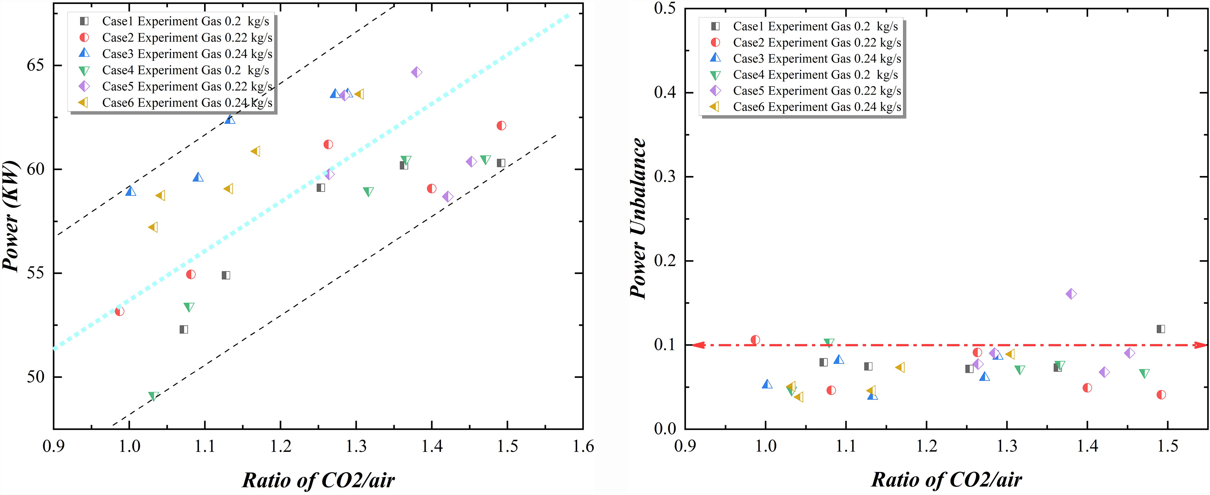
The scattering of data points in the Figure 3 (left figure) is primarily attributed to flow fluctuations on the combustion gas side, suggesting that at high temperatures, the flow rate on the combustion side may exert a more dominant influence than that of CO2. The deviation in the Figure 3 (right figure) between the heat transfer capacities of the cold and hot sides indicates that the experimental data were obtained under steady-state conditions, which will not be reiterated in subsequent analyses. The heat exchanger's power was determined by averaging the power values calculated from both the gas side and the CO2 side. The specific calculation method involved multiplying the mass flow rate by the enthalpy difference between the inlet and outlet. For the CO2 side, the thermophysical property data were obtained from the NIST REFPROP 9.1 database, while the gas-side calculations assumed a constant specific heat capacity (cp = 1.33 kJ/(kg·K)) based on textbook approximations. The deviation in heat transfer power was quantified as the ratio of the difference between the average power and the gas-side power to the average power itself.
Most of the deviations (Figure 3 right side) in heat transfer between the cold and hot sides ranged between 5 and 10%. At lower CO2/air mass ratios, the time required to reach thermal equilibrium was shorter. Due to experimental parameter fluctuations, most errors remained within 10%. However, at higher CO2/air mass ratios, the data points exhibited greater dispersion. This was attributed to the longer time required to achieve thermal equilibrium, combined with parameter fluctuations, leading to larger deviations.
Variation of total pressure loss coefficient and logarithmic mean temperature difference (LMTD)
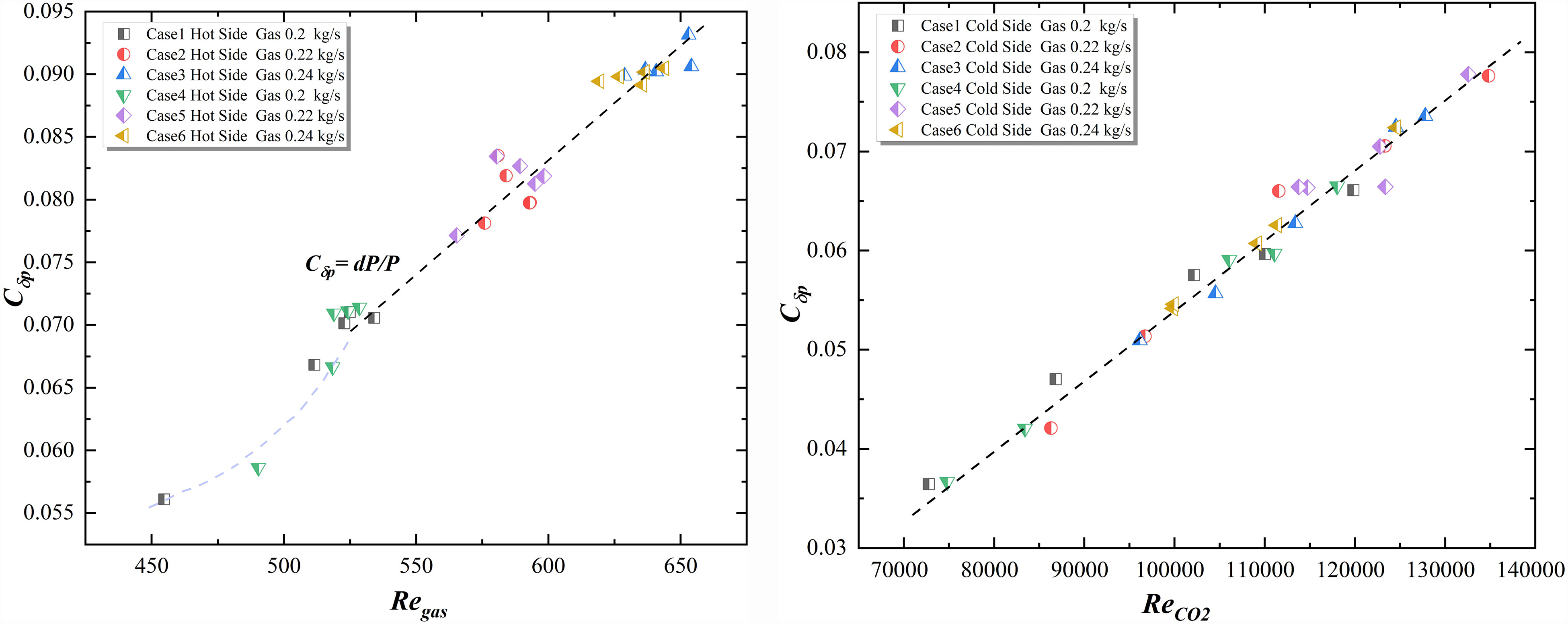
The variation of the total pressure loss coefficient generally lacks a definitive correlation with the Reynolds number (Re). However, in this study, an intriguing relationship between the two is observed. As shown in Figure 4, the trends of the total pressure loss coefficient on both the cold and hot sides are presented. On the combustion gas side (Figure 4 left), when Re < 520, the relationship follows a quadratic function, while for 520 < Re < 650, it exhibits an approximately linear correlation. According to conventional pipe flow or flat-plate flow theory, the flow under the current conditions should predominantly be laminar. Thus, the primary source of pressure loss is expected to be wall friction. Notably, under minimal fluctuations in pressure and temperature on the combustion gas side, the results demonstrate a linear dependence on velocity, closely resembling the fully developed laminar flow described by the Hagen-Poiseuille equation (Equation 1), which aligns with laminar flow characteristics.
From another perspective, assuming the empirical formula for laminar pipe flow holds and adopting the simplest treatment—where the pressure drop is normalized by the dynamic pressure at a reference temperature—substituting Equation 3 into Equation 2 theoretically yields Equation 4, which is fundamentally consistent with Equation 1. Figure 5 (left figure) confirms reasonable agreement with Equation 4. Therefore, within this narrow Re range, a theoretical solution exists when neglecting complex external flow loss mechanisms classification. However, it should be noted that the Re range in this study is limited, and the above conclusions may not be generalizable to broader conditions.
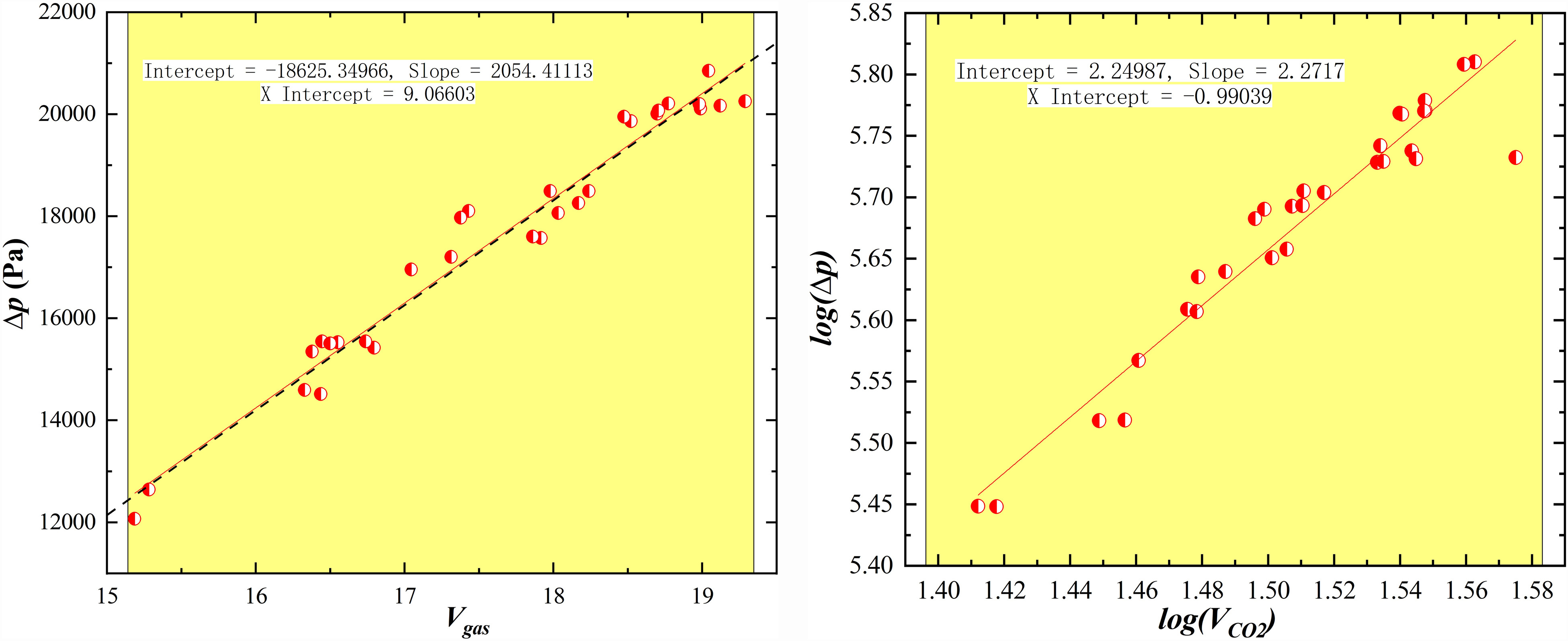
From the CO2-side results in Figure 4 (right side), within the Reynolds number (Re) range of 70,000 to 140,000, the total pressure loss coefficient exhibits a linear relationship with Re, indicating turbulent flow conditions in the pipe. First, considering the entrance length of the pipe flow, Equation 5 suggests a maximum entrance length of approximately 253 mm and a minimum of 225 mm. Given that the inlet Re significantly exceeds the critical value of 2,300, the flow is governed by turbulent inlet boundary conditions. This implies that within the 300-mm-long pipe, the influence of the boundary layer (laminar sublayer) is relatively limited.
Applying the Blasius solution for turbulent friction factor (Equation 6) to analyse the friction factor, the theoretical pressure loss versus velocity relationship should follow Equation 7. However, Figure 5 (right side) reveals an empirically fitted coefficient of 2.27, exceeding the theoretical value of 1.75. This discrepancy may be partially attributed to turbulence enhancement caused by heat transfer under supercritical conditions. This suggests that empirical correlations for flow resistance in pipes must account for additional losses arising from strongly coupled heat transfer processes with variable thermophysical properties.
According to the Moody chart (Wang, 2014), surface roughness exceeding 0.0015 times the pipe diameter would significantly influence friction factors in this Re range. In this study, the tube bundle features hydraulically smooth walls. Therefore, turbulence amplification due to temperature gradients near the heat transfer surfaces and increased turbulence-affected regions resulting from the small pipe diameter are likely dominant factors affecting the friction factor (Jackson, 2013).
As evident from Figure 6 (left side), the logarithmic mean temperature difference (LMTD) remains essentially constant during the actual heat transfer process. Even under the same gas-side Reynolds number (Re), significant variations in the CO2-side Re (i.e., flow rate) exhibit minimal influence on the LMTD. This observation suggests that the current heat transfer limitation primarily stems from the thermal resistance on the gas side. Consequently, the gas-side heat transfer coefficient emerges as the critical factor governing the overall thermal performance of the precooler. Further explanation is provided as follows:
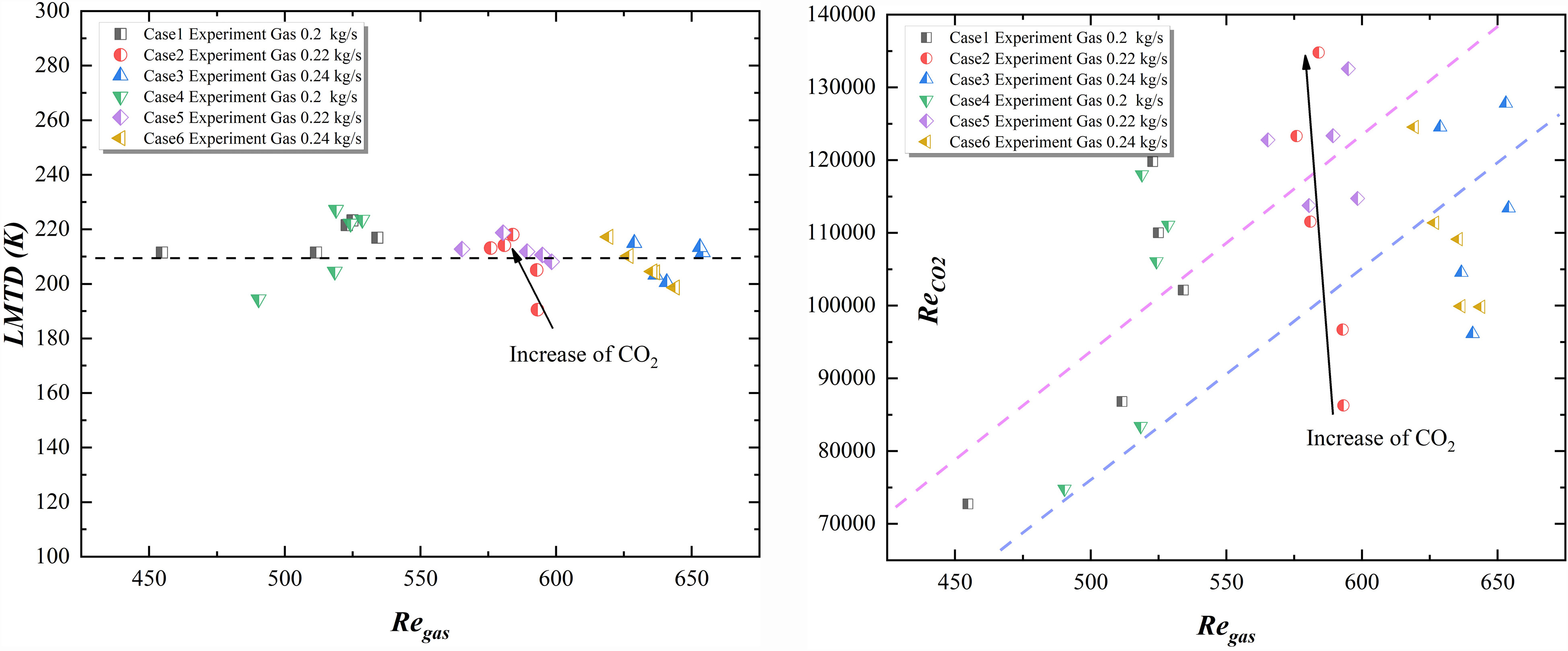
The right panel of Figure 6 illustrates the variation in the Reynolds number (Re) of the cold-side supercritical CO2 corresponding to the gas-side Reynolds number range (Re: 450–650). Taking Case 3 as an example, while the gas-side Reynolds number remains constant, the CO2-side Reynolds number increases from 9,300 to 13,000. However, the left panel of Figure 6 demonstrates that the corresponding logarithmic mean temperature difference (LMTD) remains essentially stable at 210 K, with a variation of less than 5%. Consequently, the change in CO2 conditions exerts minimal influence on the temperature potential field. This observation will be further elucidated in Figure 7, which examines the impact on the overall average heat transfer coefficient.
The distribution of the overall average heat transfer coefficient (UA)
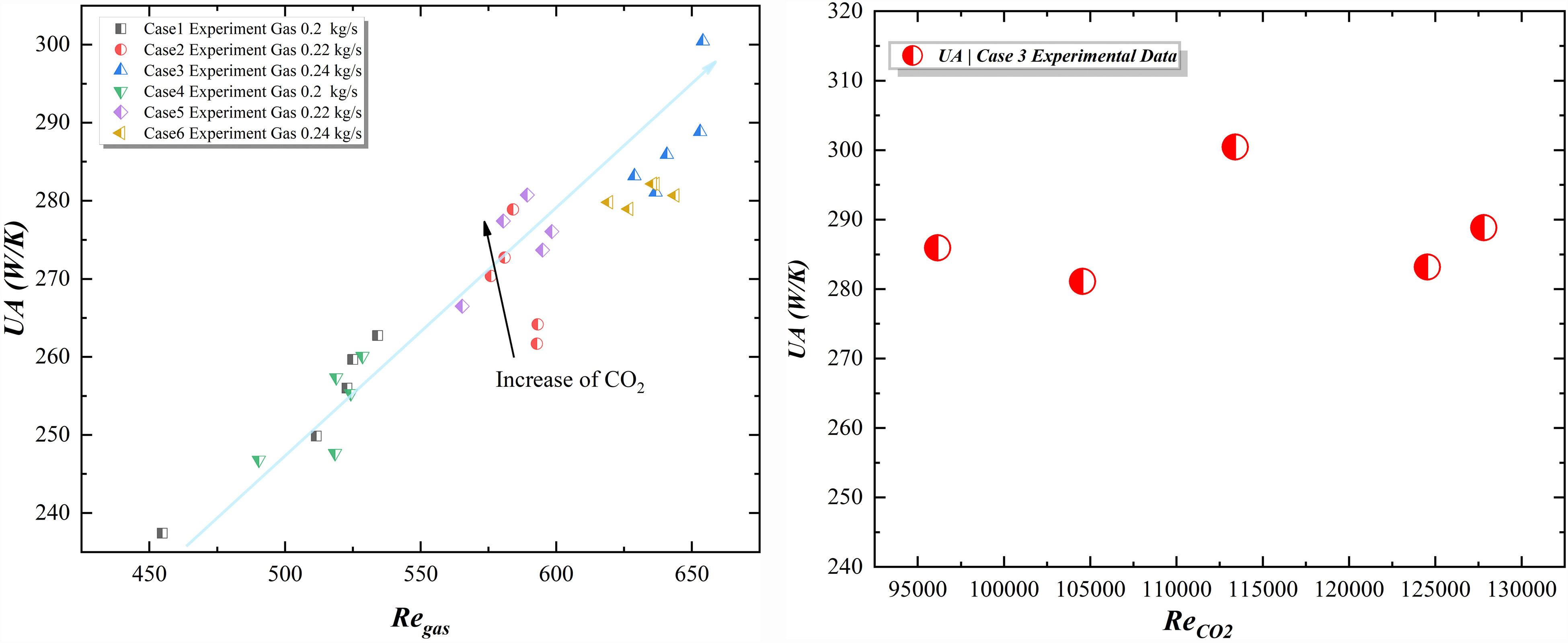
As illustrated in Figure 7 (left panel), the overall average heat transfer coefficient (UA) increases with the rising Reynolds number (Re) on the gas side, exhibiting an approximately linear trend. This observation further corroborates the conclusion derived from Figure 6—that the gas-side heat transfer coefficient is the dominant factor limiting the thermal performance of the precooler.
Although the analysis of Case 3 (arrows in left panel) indicates that the cold-side Re number contributes to enhanced heat transfer to some extent, the primary governing factor remains the hot-side (gas-side) Re number. This is evident from the magnitude of variation in UA, which is predominantly influenced by the thermal-side conditions. The right panel of Figure 7 illustrates the relationship between the UA value and the cold-side Reynolds number (Re) in Case 3. It can be clearly observed that, regardless of the variation in the CO2-side Re number, the overall average heat transfer coefficient fluctuates around 290 K without exhibiting a distinct linear or exponential correlation. Combined with the results from the left panel of Figure 7 and the corresponding findings in Figure 6, this suggests that the convective heat transfer capability on the gas side is the primary limiting factor governing the performance of the precooler.
Design and evaluation methodology for the precooler
The design and evaluation methods of the precooler share a fundamentally similar computational framework. The design method involves determining the detailed geometric configuration of the heat exchanger based on thermodynamic performance requirements, given a predefined basic heat exchanger type (or, in practical applications, a minimal periodic geometric structure). This process includes iterative geometric adjustments to simultaneously meet both heat transfer and flow resistance constraints, followed by structural strength validation.
Conversely, the evaluation method operates under known geometric conditions, computing the outlet temperature and thermal efficiency of the heat exchanger based on inlet parameters. This requires iterative calculations of the outlet temperature until a steady-state solution is achieved. Both approaches rely on dimensionless correlations governing heat transfer and flow resistance as their computational core. To enhance accuracy, a discretized sub-heat-exchanger approach is typically employed, wherein thermophysical properties within each sub-unit can be approximated as varying linearly. This mitigates significant errors in logarithmic mean temperature difference (LMTD) calculations under strong property variations.
Given that the feasibility of the design method can be indirectly validated by the precision of the evaluation method, the present study focuses exclusively on the latter, omitting further elaboration on the design process.
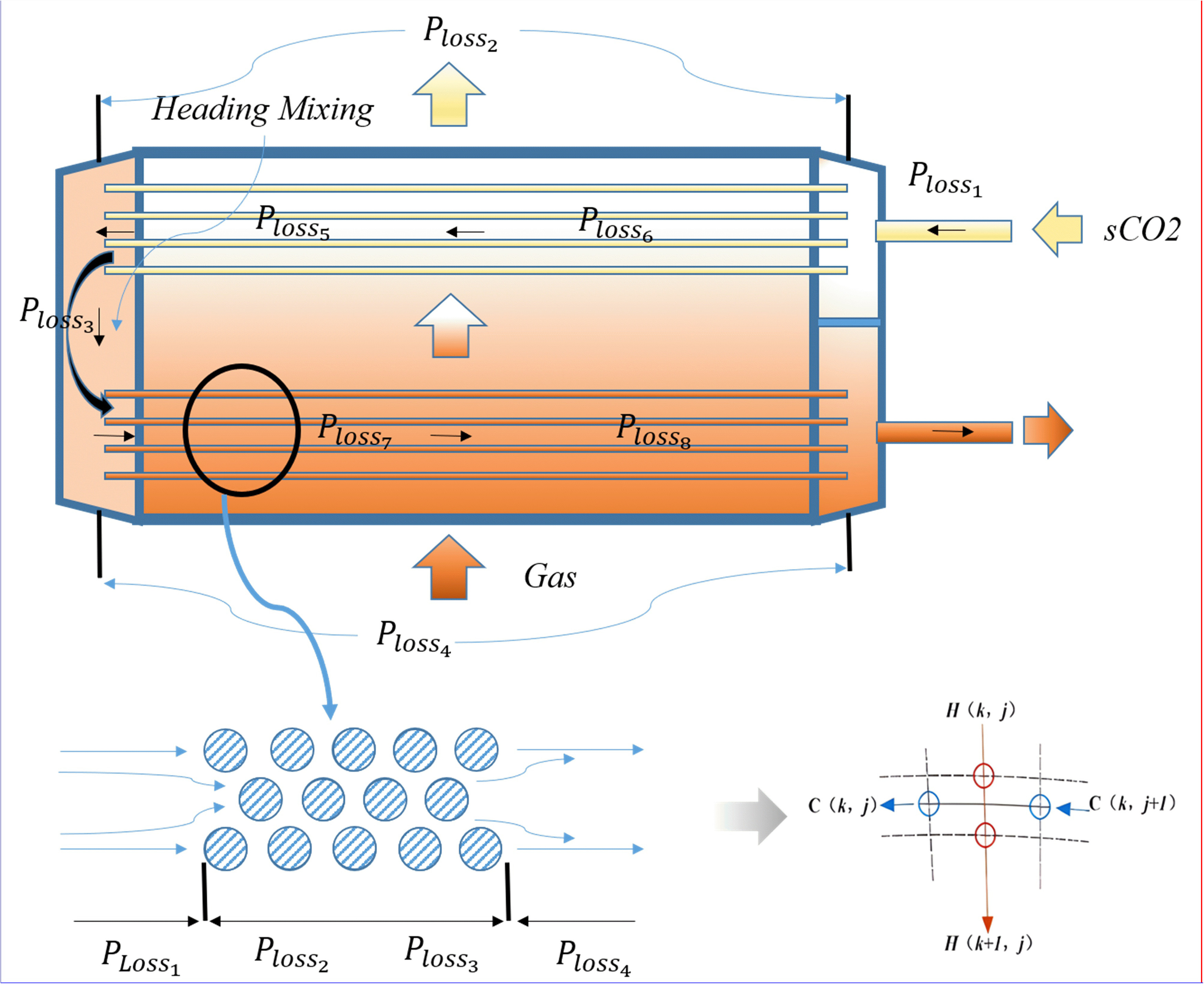
This study employs the flow resistance separation model proposed by Kays and London (1984) for theoretical analysis. As illustrated in Figure 8, the flow losses on the gas side primarily consist of inlet contraction loss, outlet expansion loss, as well as core friction loss and acceleration loss in the intermediate section. On the CO2 side, the situation is more complex, incorporating additional header loss. Furthermore, since the capillary tube bundle is divided into front and rear sections, the flow resistance losses must be evaluated separately. Two key assumptions are adopted: first, the mixing temperature is approximated as the arithmetic mean of the inlet and outlet temperatures; second, the outlet header loss is neglected by default.
Design framework with experimental data-driven performance calibration
In the preceding analysis, this paper have established that the convective heat transfer coefficient on the gas side significantly influences the accurate evaluation of heat exchange capacity, while the friction factor on the CO2 side deviates from conventional analytical solutions. Therefore, this study primarily focuses on these two aspects and proposes a design correction methodology based on experimental data, as illustrated in Figure 9.
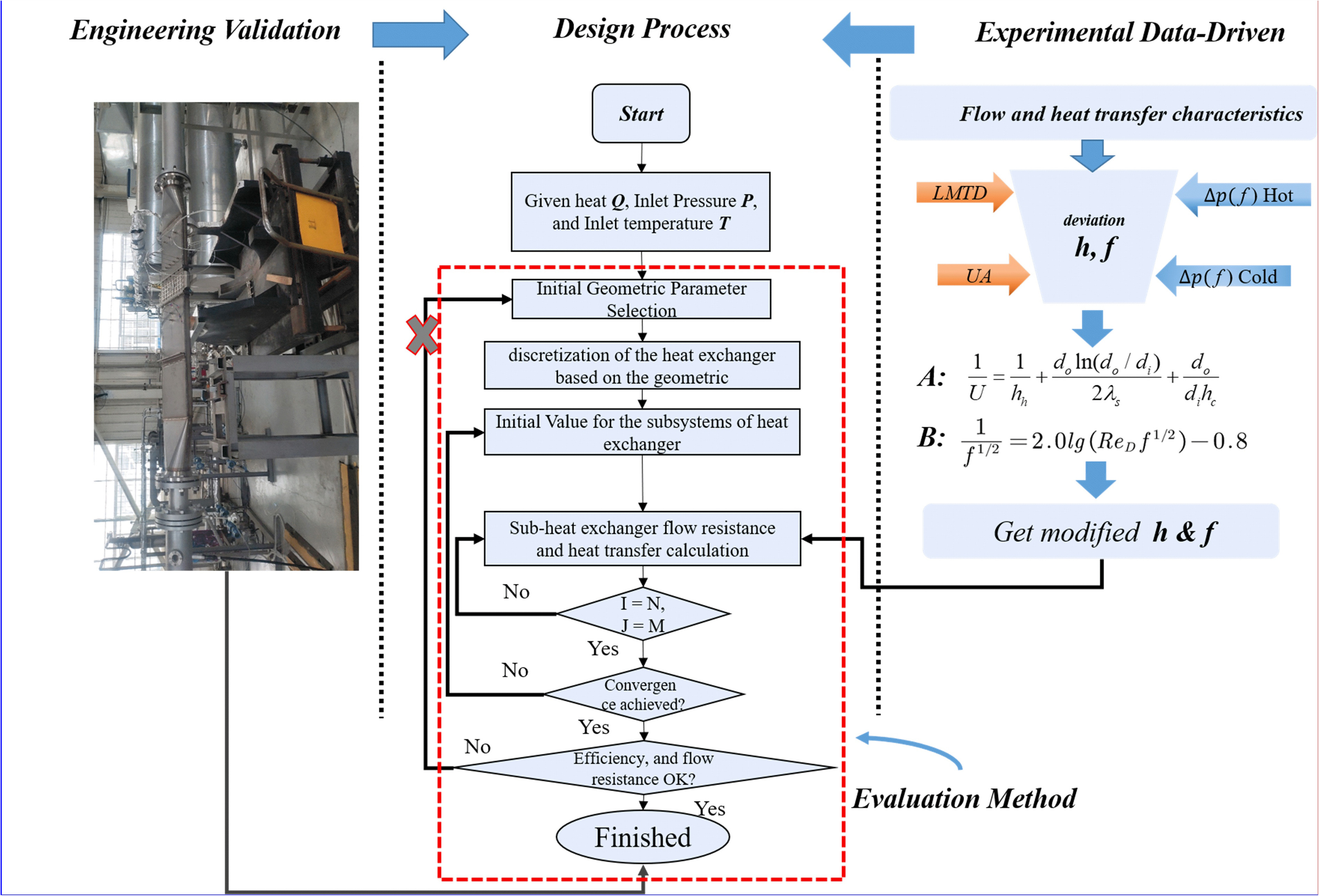
For calibrating the hot-side heat transfer coefficient, given the abundance of mechanistic experiments and data on supercritical CO2 in micro-tube bundles—which are already well-established—we directly adopt Jackson's low-dimensional predictive model (Jackson, 2013) for the cold side. Regarding cold-side flow resistance, the reduced tube diameter and coupled heat transfer effects induce near-wall flow structures resembling rough particle interactions. Consequently, this study derives an empirical correlation for the Reynolds number exponent (approximately 0.2717) through comparative analysis of experimental data and theoretical predictions, followed by coefficient fitting.
The hot-side flow resistance aligns well with theoretical solutions, so the well-validated empirical correlations for staggered tube bundles (e.g., (Kays and London, 1984)) are retained without modification. Upon obtaining the corrected hot-side Nusselt number (Nu) and cold-side friction factor (f), a two-dimensional discretized sub-heat exchanger model is employed for numerical evaluation, followed by comparison with experimental validation data.
Mathematical framework for performance evaluation
For detailed explanations of the formulas in Table 4, please refer to Reference (Tang et al. 2023).
Table 4.
Flow resistance loss separation model based on Figure 8.
In the context of supercritical CO2 internal flow heat transfer models for micro-tube bundles, Equation 20 indicates that there are explicit constraints among the total average heat transfer coefficient, the thermal conductivity of the capillary tube bundle, and the convective heat transfer coefficients of the internal and external flows. The total average heat transfer coefficient was determined experimentally, the thermal resistance of the solid was obtained from material properties, and the internal flow convective heat transfer coefficient was derived from empirical correlations. Thus, the convective heat transfer coefficient of the external hot flow and the corresponding low-dimensional Nusselt number model could be determined.
Results and discussion
In this study, the Nusselt number (Nu) on the gas side and the friction factor (f) on the CO2 side were empirically correlated with the Reynolds number (Re) and Prandtl number (Pr) based on experimental data. When modifying the CO2 friction factor, it was inferred from previous analysis that surface roughness likely plays a role, possibly due to turbulence-induced flow structures, which are themselves influenced by heat transfer. Therefore, the Prandtl number was also incorporated to account for convective heat transfer effects. The original semi-empirical Prandtl correlation (Wang, 2014) does not consider roughness effects, so the empirical correlation by Paalanen, which shares a similar form, was selected as a reference and subsequently modified. The final results are presented in Equations 23–25.
As shown in Figure 10, the predicted values of the heat-side heat transfer coefficient, modified based on experimental data, exhibit good agreement with the measured values. However, since the properties of air from NIST (Lemmon, 2002) were used in this study to approximate those of the actual fuel gas, the overall predictions tend to be slightly overestimated, and the intermediate parameter variations are not fully captured.
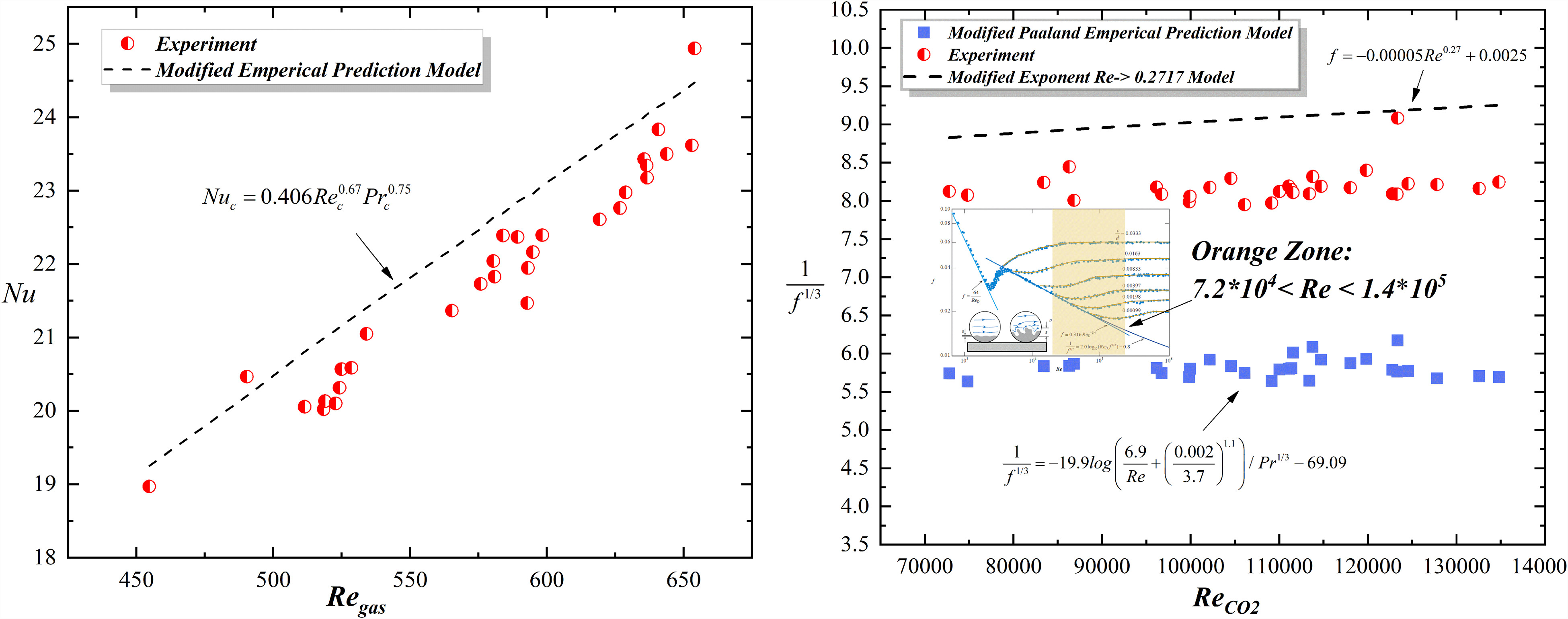
Similarly, predictions based solely on a power-law relationship with the Reynolds number (Re) show reasonable overall agreement but fail to adequately reflect property variations and generally underestimate the results. In contrast, the modified correlation incorporating roughness and the Prandtl number (Pr) better captures property-dependent variations but yields systematically higher values. Therefore, a more balanced and accurate prediction may be achieved by taking the average of the two approaches.
In this study, a co-current flow arrangement was adopted for two-dimensional discretization. Compared to a counter-current flow configuration, the co-current layout leads to a larger discrepancy between the predicted and experimental values of the outlet temperature difference.
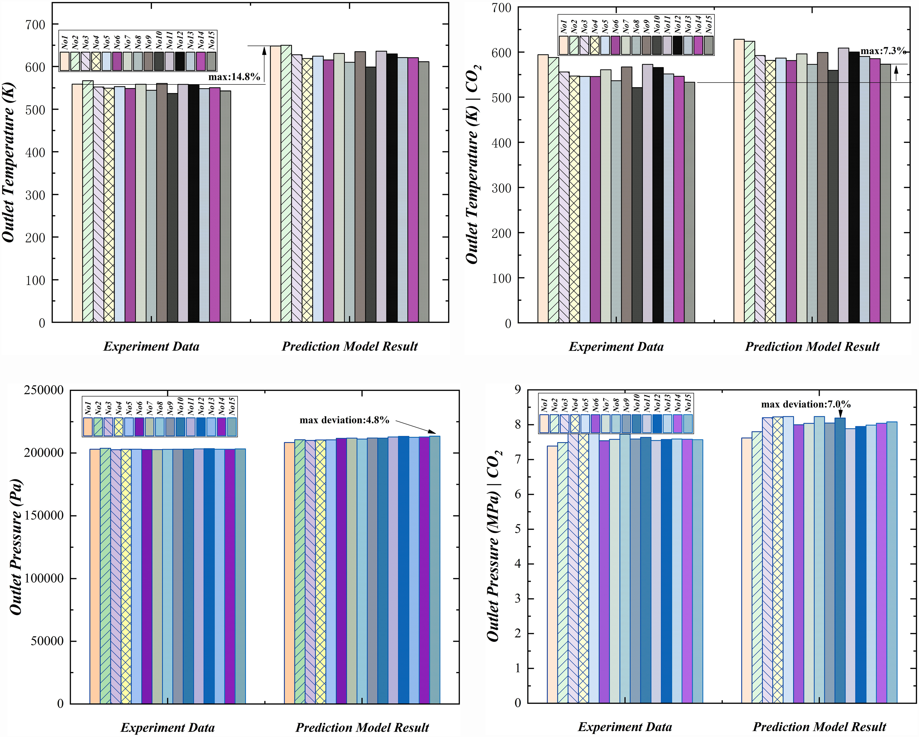
As illustrated in Figure 11, the comparison between the model predictions (modified based on experimental data) and actual experimental values reveals a maximum deviation of 14.8% for the air-side outlet temperature and 7.3% for the CO2-side temperature. Additionally, the maximum deviations in outlet pressure are 4.8% for the air side and 7.0% for the CO2 side. These results indicate that the predictive model achieves reasonable accuracy. Subsequent verification using a counter-current flow arrangement is expected to further reduce deviations, demonstrating that the data correction method and results presented in this study possess significant reference value.
However, the findings of this study are still not entirely mature at present. The following discussion elaborates on this point:
Point 1: deviation in CO2-side flow resistance and heat transfer correlation
The study observed that the flow resistance coefficient on the CO2 side deviates from classical interpretations. According to the Chilton-Colburn analogy, the empirical correlation for the convective heat transfer coefficient (or Nusselt number, Nu) should also exhibit a corresponding deviation (i.e., Nu ∼ f, where f is the friction factor). However, in this work, the Jackson et al. correlation (originally developed for supercritical CO2 convective heat transfer in tubes) was directly applied without accounting for this deviation. Future studies should refine the model to incorporate this discrepancy and improve accuracy.
Point 2: gas-side flow resistance and heat transfer characteristics under compact heat exchanger
Experimental results indicate that the gas-side flow resistance coefficient aligns well with classical pipe flow friction correlations (e.g., Moody chart). However, due to the high compactness of the heat exchanger, its heat transfer mechanism resembles that of a porous medium heat exchanger. Despite low flow velocities and small Reynolds numbers (Re), the heat transfer performance remains strong, which we tentatively attribute to “size effects” in this study. The gas-side heat transfer coefficient emerges as the dominant constraint in the system. Increasing the CO2 flow rate provides less heat transfer enhancement compared to increasing the gas-side flow rate, suggesting that: The gas side acts as the “master switch” (controlling overall heat transfer) and the CO2 side acts as a “sub-switch” (secondary influence). This observation further supports the deviation from the Chilton-Colburn analogy, reinforcing the second major uncertainty in this study.
Under the observed deviations (gas-side “size effects” & CO2-side Chilton-Colburn analogy breakdown), existing predictive models (e.g., empirical correlations, CFD simulations) may fail to accurately capture the actual heat transfer and flow resistance behaviour. Given these uncertainties, direct calibration using experimental data is adopted in this study to ensure robustness. This approach compensates for the limitations of conventional models, particularly in highly compact heat exchangers. The flow and heat transfer mechanisms in ultra-compact precoolers remain partially unresolved, necessitating: further theoretical investigations and multi-fluid experimental validation.
From the perspective of the actual flow and heat transfer mechanisms and their coupling processes, the framework in this study remains unchanged, but the specific calculation methods within the framework can be modified. The current results are based on the assumption of parallel-flow heat exchange, and their limitations stem from the following aspects:
The predictive model adopts the assumption of parallel-flow heat transfer. In reality, if counter-flow heat exchange were applied, the deviation could likely be further reduced.
However, in practical computations, when multiple sub-heat exchangers are configured, the solution tends to diverge easily and requires excessive computational time, which remains an issue to be resolved.
Nevertheless, this study found that, for this specific heat exchanger configuration, the parallel-flow assumption still exhibits reasonable accuracy, suggesting that the staggered tube bundle flow pattern may have a more significant influence than the relative flow direction of the hot and cold sides.
Summary
Although this study aims to enhance the precision of the design methodology, it does not directly validate the design method itself. Instead, by examining the core computational principles shared between the design and evaluation methods, it reveals that both approaches fundamentally rely on the same critical calculations. Consequently, the primary objective of this work—the development of a data-driven design methodology—is inherently centered on the accuracy of the evaluation model, with both methods adhering to the same precision criteria.
Through theoretical analysis and experimental data, this study identifies the convective heat transfer coefficient on the gas side and the pressure loss coefficient on the refrigerant side as the primary sources of uncertainty in the current evaluation method. The following empirical correlations were derived and validated through independent experiments, demonstrating excellent applicability within the investigated Reynolds number range.
The maximum deviation of the air-side outlet temperature was 14.8%, while that of the CO2-side temperature was 7.3%. The maximum deviation of the air-side outlet pressure was 4.8%, while that of the CO2-side pressure was 7.0%.