Introduction
Unmanned Aerial Systems (UAS) are attracting significant attention in aerospace research and development as a result of their wide range of applications in various aerospace fields (Chahl, 2015). In military applications, efforts are being made to fully integrate propulsion systems into the aircraft fuselage (Johansson, 2006). Highly bent intakes offer significant advantages because their small size allows close integration into the fuselage, while also reducing structural weight and preventing radar reflections from the fan. Using complex, S-shaped intake systems with strong curvature, however, presents a challenge in terms of total pressure and swirl distortion, resulting in reduced engine performance and stability limitations (Rademakers et al., 2016; Migliorini et al., 2023). Callahan and Stenning (1971) investigated the effects of a compressor system on static pressure distortions caused by a screen in the inflow. Other studies have shown that the total pressure distortion are relatively constant when influenced by the compressor (Soeder and Bobula, 1979). The impact of steady-state flow distortion gained significant focus over the years (Haug and Niehuis, 2017; Haug et al., 2018; Maghsoudi et al., 2020). Transient total pressure distortion in intake systems was first found to be critical to aircraft engine performance early in fighter aircraft engine development. The study identified engine stall as a potential result of time-dependent distortion (Bowditch and Coltrin, 1983). Challenges that emerged in the development cycle of a series of aircraft led to significant efforts to characterize such intake flows and understand engine response. Flow distortions can arise from a wide range of aerodynamic effects, such as boundary layer ingestion or secondary internal flows. General aircraft intakes and S-shaped ducts in the context of flow distortion quantification has been investigated in a wide range of research. Previous studies demonstrated that total pressure distortion with the interacting counter-rotating vortex systems significantly reduces the surge margin and stability of the engine (SAE International, 2022). Local maxima of parameters to quantify the flow distortions had a significant effect on the engine (Stevens et al., 1978). Unsteady distortion analysis revealed that peak radial and circumferential distortions were not synchronous, requiring both to be evaluated (Tanguy et al., 2018). Migliorini et al. (2024) showed that flow separation at the second bend of the S-shaped diffuser significantly affects the swirl distortion and exhibits strong low-frequency oscillations, which are tied to the shedding of secondary flow structures. The Society of Automotive Engineers (SAE) developed a series of indices to quantify the effects of total pressure loss and the flow distortion pattern at the Aerodynamic Interface Plane (AIP) (SAE International, 2017). The presence of highly unsteady flows in complex S-ducts (Berens et al., 2014) and the importance of dynamic distortion on the fan response (Bowditch and Coltrin, 1983) have challenged the limitations of conventional flow distortion determination methods. Furthermore, a study showed that approaches based on stationary Reynolds Averaged Navier Stokes (RANS) simulation models ignore necessary aerodynamic effects (Fiola and Agarwal, 2015). It is difficult to accurately predict the onset and extent of flow separation, especially in areas with high pressure gradients and strong curvature. A study by Piovesan et al. (2024) showed that current turbulence models may have limitations in accurately capturing unsteady flow features when analyzing unsteady aerodynamic behavior in S-ducts.
In this study, high-resolution Unsteady (U)RANS simulations, based on experimental studies (Rademakers et al., 2024) are carried out. A comprehensive simulation model combining the Low Pressure Compressor (LPC) and the intake system reveals the LPC’s steady-state and unsteady influence on the intake. Advanced distortion descriptors in combination with standard SAE parameters enable the analysis of complex phenomena. The main contributions of this work are:
Introduction of physically motivated distortion descriptors capable of resolving secondary-flow-driven unsteadiness.
Quantification of modal frequency shifts caused by LPC upstream interaction.
Demonstration of limitations of DC60/SC60 for dynamic distortion assessment.
Analysis of axial-position effects between DOP and AIP.
Methodology
Intake and engine model
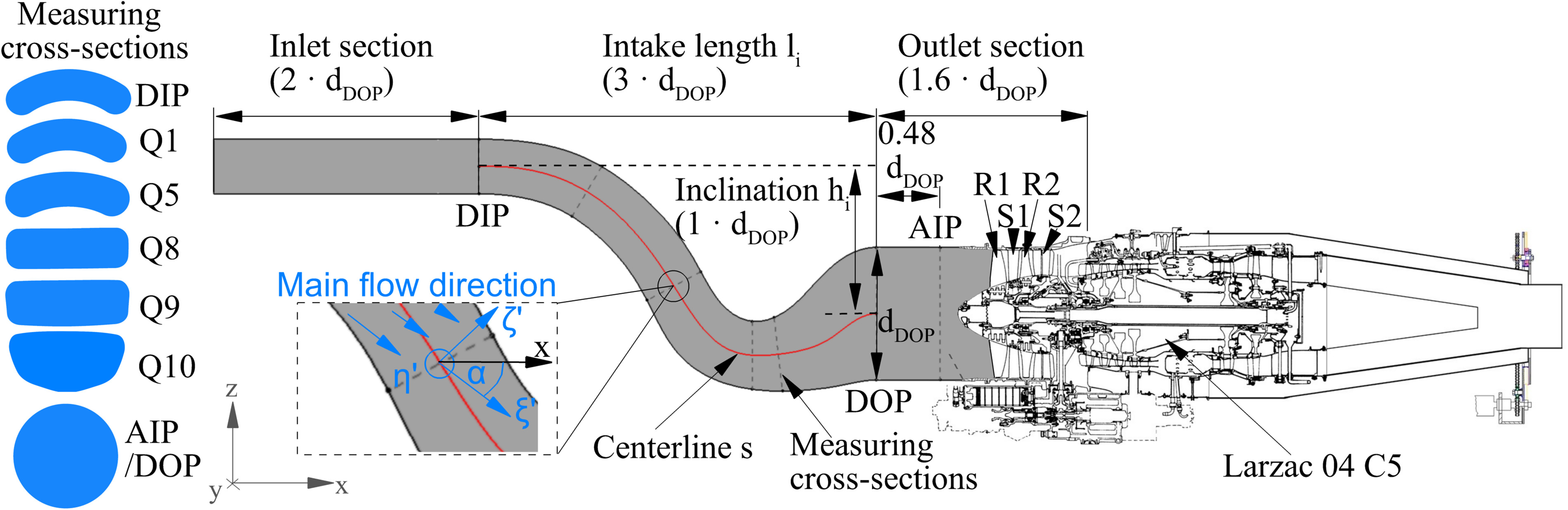
The model used for the numerical investigations consists of the highly bent intake duct Military Engine Intake Research Duct (MEIRD) and the jet engine Larzac 04 C5. It focuses on analyzing flow distortions and the interaction with the engine’s LPC. The engine’s robust design and its unmixed nozzle enable extensive throttling of the LPC (Rademakers et al., 2024). It is a turbofan engine with core and bypass mass flow divided downstream of the LPC. The LPC has two stages (R1 [x23], S1 [x61] and R2 [x29], S2 [x43]) with a tandem stator (S2) in the second stage (Figure 1). Both rotor stages are in a fully subsonic relative flow regime up to a relative spool speed of nred,rel=81%. Technical data of the Larzac engine and a comprehensive performance analysis can be found in Scheibel et al. (2024) and Stößel (2017).
Figure 1.
Scheme of the coupled configuration of MEIRD and Larzac 04 C5.
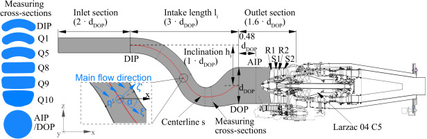
The compact intake duct design offers flexibility for integrity aircraft and intake systems requiring more space for cargo or technical equipment, such as UAS. The highly bent MEIRD is a test case for academic research. A real flight application is not desirable with this design. Rather, extreme flow behavior can be investigated. The MEIRD has an outlet diameter of dDOP=0.454 m (Duct Outlet Plane (DOP)) and an axial length of 3⋅dDOP, with the AIP located 0.48⋅dDOP downstream of the DOP (Figure 1). The duct features an outlet area (DOP) to inlet area ratio (Duct Inlet Plane (DIP)) (ADOP/ADIP) of 1.17. The inlet (2⋅dDOP) and outlet sections (1.6⋅dDOP) specify the extent of the numerical domain. In the coupled setup, the LPC is located at the rear of the outlet section. The intake system is defined by a global coordinate system (x,y,z) and an additional local coordinate system (blue, ξ,η,ζ) at the respective cross-sections (Q), which is aligned with the local main flow direction. This enables an advanced determination of more complex distortion descriptors in the later analysis. Due to the double S-shape, there is no direct line of sight from the DIP to the DOP to prevent radar-reflections from the LPC. The cross-sections change from a kidney shape at the DIP to a square at the lowest position (Q8) and back to a round shape at the DOP (Figure 1).
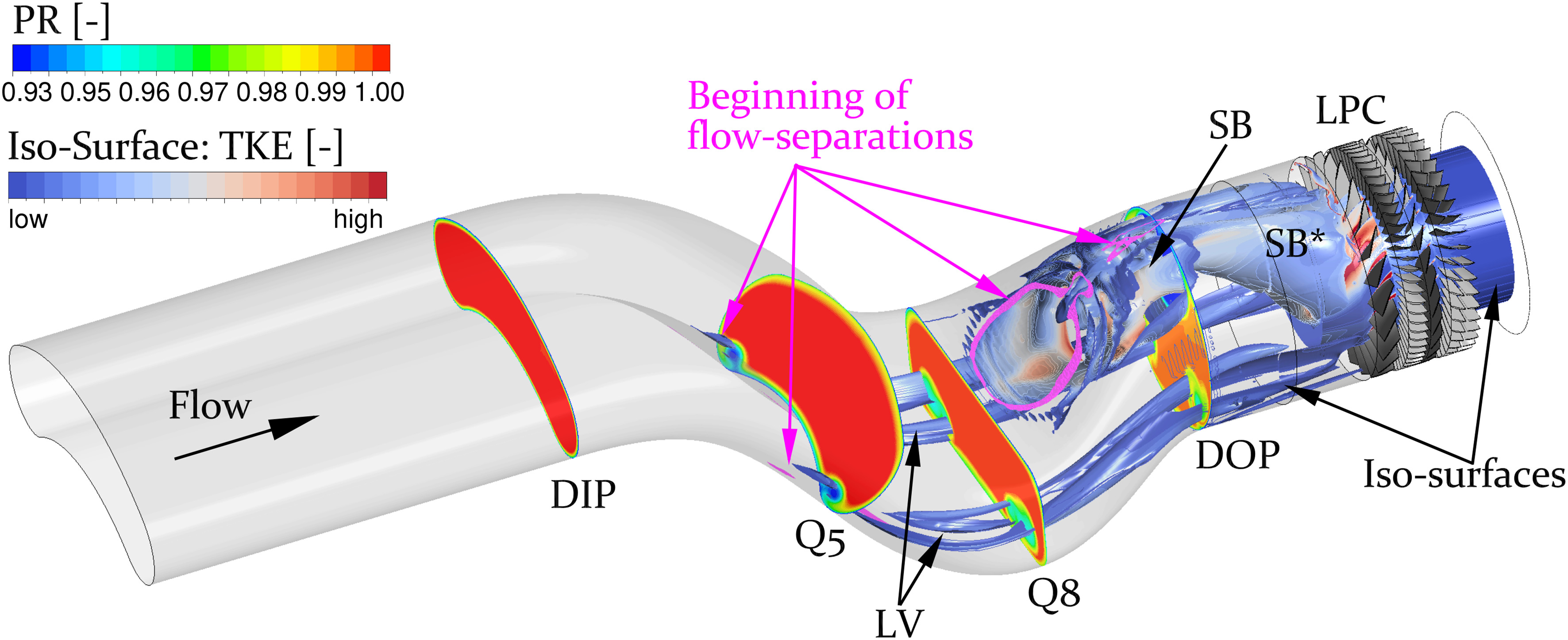
A pair of Lateral Vortices (LV) forms near cross-section Q5, which arise from the low-energy fluid from the thickening boundary layer and the kidney shape at the inlet. The flow, accelerated by the strong curvature near cross-section Q8, causes strong pressure gradients and a strong central flow separation (Flow Separation Bubble (SB)). The result is a complex interacting vortex system, causing strong flow distortions and separations, negatively affecting the engine’s performance. A comprehensive flow analysis along with phenomenological descriptions can be found in the work of Hanrahan et al. (2025) and Grois et al. (2023, 2024).
Numerical modeling
In this study, steady-state and unsteady RANS Computational Fluid Dynamic (CFD) simulations were performed to predict the flow of a fully coupled intake and LPC system and an isolated intake model. The steady-state simulations are used as the initial solution for the unsteady simulations and as stationary comparative data for the results. The simulations were carried out using ANSYS CFX with Menter’s k-ω-SST turbulence model (fully turbulent flow) with the additional option of curvature correction to reduce two-equation model problems with streamline curvature (Spalart-Shur) (Smirnov and Menter, 2009). Previous studies have shown the capability of calculating non-uniform duct flows with these modelling approaches (Brehm et al., 2014). A high-resolution second-order scheme was used to discretize the advection term, and a second-order backward Euler scheme was used to solve the transient terms. The inlet conditions were defined by pt and Tt. The S2 outlet was described by the Exit Corrected Mass Flow (ECMF). Due to the asymmetric intake flow distortion propagated through the LPC stages, pressure outlet conditions with radial equilibrium or averaging over the entire outlet have proven to be more unstable over extremely long periods in unsteady simulations. Both Mixing Plane (MP) and Frozen Rotor (FR) interfaces (intake to spinner, spinner to R1, R1 to S1, S1 to R2, R2 to S2) were selected for the steady-state simulation. Transient interfaces were chosen for the unsteady simulation to fully capture the upstream effect of the LPC. The operating point investigated corresponds to a relative spool speed of nred,rel=76% (≃13,667 RPM) in a subsonic flow regime on the test bench under ambient conditions (Tt,In=303.15 K and pt,In=94,217 Pa). The unsteady simulation’s time step was defined as 1∘ of the LPC rotation (Δt=1.22⋅10−5 s). This also allowed adequate convergence (momentum and mass residual (RMS) value ≤1⋅10−5) to be achieved with reasonable computational costs (max. at 25 inner loop iter., criterion usually fulfilled after 6–10 iter.), while also covering the sampling rate required for later analysis and the modes occurring in the duct flow. The investigation of unsteady phenomena of the LPC flow is not part of the work and would require a smaller time step. The simulations cover a total of 100 LPC rotations.
The selected blade’s geometry is based on a former fluid-structure interaction (FSI) steady-state RANS simulation with ANSYS CFX to determine the LPC’s performance shift (Scheibel et al., 2022). The meshes used in this study are based on the resulting geometries. The results provided information on the stationary deformation of R1 and R2 as a function of the spool speed and throttle state. It showed a maximum deformation of 3.82 mm and a tip stagger angle change of 0.4∘ at a relative spool speed of nred,rel=76%, significantly affecting the LPC’s performance. The dynamic influence of the FSI was neglected.
Meshing and convergence control
The block-structured meshes for the intake and the spinner were generated using ANSYS ICEM with a central H-block and an outer O-grid for wall resolution. The LPC’s blade mesh was generated by ANSYS TurboGrid. The wall refinement allows a low Reynolds number treatment and a dimensionless wall distance of y+≤1. The mesh-independence study focuses on the influence of the LPC on the intake. Therefore, different LPC meshes were evaluated. Mesh studies already exist for the MEIRD. In an initial mesh convergence study of the isolated intake, a mesh element number of 4 million was found to be adequate for flow prediction (Haug and Niehuis, 2017). More recent studies with a focus on detailed turbulence modeling required higher mesh element numbers (Hanrahan et al., 2025). Therefore, high-resolution intake and spinner mesh with 23.2 million and 7.6 million mesh elements will be used without change (L1, M1, H1, H2) for the mesh convergence study done in this work. For analyzing the influence of coupled intake and LPC, mesh M2 uses a coarser intake mesh with 4.2 Mio and a spinner mesh with 1.9 Mio mesh elements. The simulation domain consists of the full annulus LPC. The LPC’s mesh element size is changed globally (total mesh elements, Mio.: L1: 91.2, M1: 137.7, M2: 113.0, H1: 210.8, H2: 270.2).
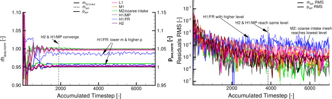
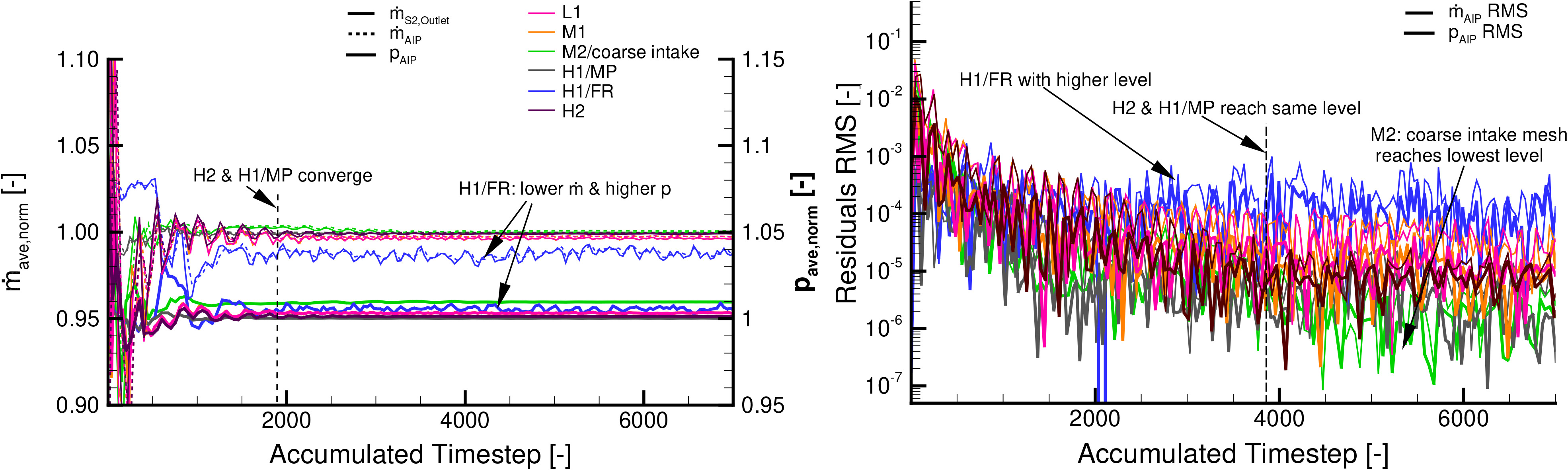
The mesh convergence study is based on the steady-state simulations. Additional convergence criteria for monitoring the area averaged pressure (p¯AIP|S2Out) and mass flow (m˙AIP|S2Out) fluctuation at AIP and the S2 outlet were defined (Figure 2, left). Mean square residuals (RMS) were obtained at AIP (Figure 2, right). A total of 10,000 iterations were run for the study; Figure 2 show a sample of 7,000 iterations. The global convergence criterion was set to 1⋅10−5. The convergence criterion for normalized pressure and mass flow fluctuations was 0.0005. A FR and a MP with the H1 mesh were also investigated to see the effect of asymmetric flow distortions or the radial averaging of the intake flow to the steady-state LPC. The meshes M1, H1/MP, and H2 have only a minor impact on pressure and mass flow fluctuations at the AIP and the S2 outlet. The H1/FR mesh shows a lower (m˙AIP|S2Out) and a higher (p¯AIP|S2Out) at the AIP and the S2 outlet. The coarsest mesh L1 shows only deviations with the pressures. The M2 mesh with low-resolution intake and spinner mesh shows a large pressure difference at the AIP. The H2 and H1/MP meshes show well-converging characteristics after 1,850 iterations, and mesh H1 was finally chosen. The isolated MEIRD configuration with the 23.2 million mesh reached the convergence criteria more quickly. Continued and not fully converging pressure fluctuations are caused by the highly unsteady flow behavior of the MEIRD. This is acceptable, as the convective flows between duct and LPC under the influence of flow distortions are crucial for the coupled setup. The results of the steady-state mesh convergence study are applied to the URANS mesh and simulations.
Figure 2.
Mesh convergence study, averaged (normalized) pressure (p¯AIP|S2Out) and mass flow (m˙AIP|S2Out) at AIP and the S2 outlet (left), RMS residuals at the AIP (right).
Validation of the numerical model
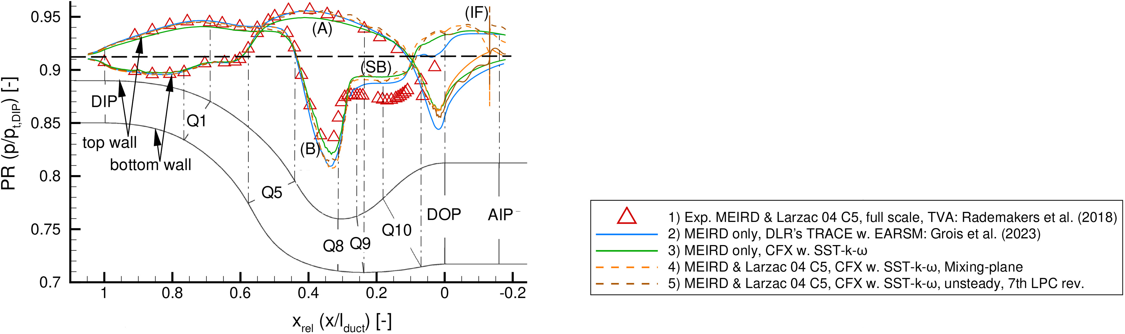
The wall pressures resulting from the simulations are compared with experimental data from a previous study of the coupled MEIRD and Larzac 04 C5 engine (Rademakers et al., 2024). Figure 3 shows the Pressure Recovery (PR) (p/pt,DIP) related to the inlet conditions and a scheme of the MEIRD with the named cross-sections. In addition, the results are compared with an existing and well-known setup using the DLR’s flow solver TRACE and the Hellsten explicit algebraic Reynolds stress (EARSM) turbulence model (blue), (2) (MEIRD only, DLR’s TRACE w. EARSM) (Grois et al., 2023). (2) shows a good correlation with the exp. wall pressures. Differences are observed in the central flow separation (SB) region. More significant differences are shown by simulations (3) (MEIRD only, CFX w. SST-k-ω), (4) (MEIRD and Larzac 04 C5, CFX w. SST-k-ω, MP), (5) (MEIRD and Larzac 04 C5, CFX w. SST-k-ω, unsteady, 7th LPC rev.), which rely on CFX and k-ω-SST turbulence model.
Figure 3.
Wall pressure profile of the MEIRD, comparison of exp. (Rademakers et al., 2018) and num. data, isolated intake vs. coupled intake and engine.
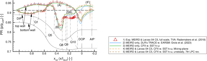
Near (A), a deviation to the experimental data is given by the isolated MEIRD simulation (3), which does not occur in the coupled simulations (4) and (5). The coupled CFD and TRACE simulations similarly predict the lowest peak (B). The positioning of the interface between the spinner and the intake (IF) results in a discontinuity of the wall pressures. Finally, the CFD models show a good correlation with the experimental data. Areas of strong flow separation are not accurately reproduced but modeled qualitatively. Further detailed num. and exp. wall pressure data can be found in (Hanrahan et al., 2025).
Distortion descriptors
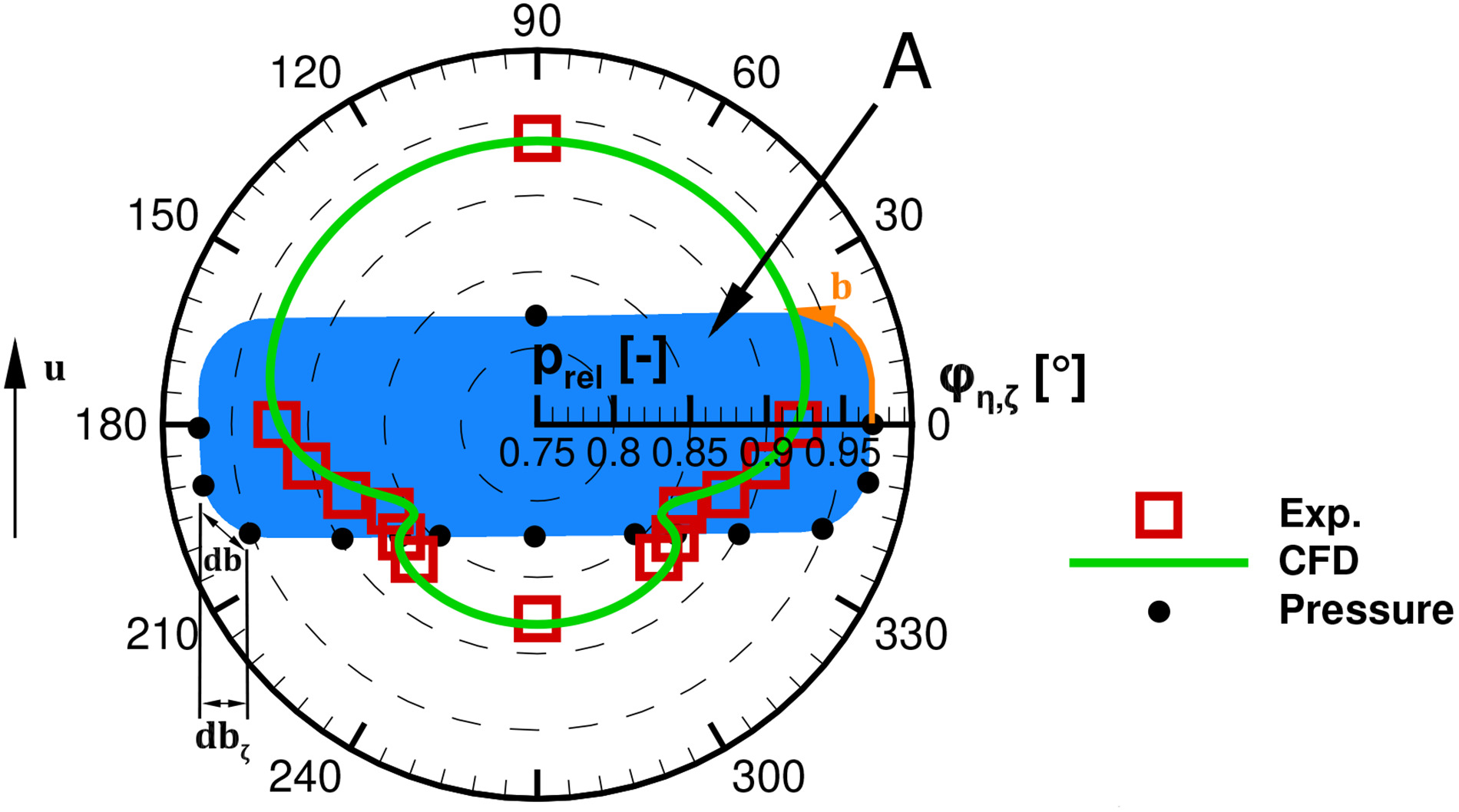
The distortion descriptors quantitatively describe the flow inhomogeneity on the engine and intake interfaces. The parameters have been determined at the cross-sections marked in Figure 1 (see also (Grois et al., 2024)) as surface integrals (A) or as integrated circumferential (b) pressure value (see Figure 4). In this paper, parameters at the DOP and AIP are considered. In addition to traditional distortion descriptors, such as DC60 und SC60 (SAE International, 2011), advanced parameters are also discussed. The additional parameters react differently to various aerodynamic phenomena and offer significant advantages compared to traditional turbomachinery parameters (Grois et al., 2023). Coefficients are used to correlate the values.
Figure 4.
Determination of the cross-sectional flow inhomogeneity parameters, example: cross-section Q8.
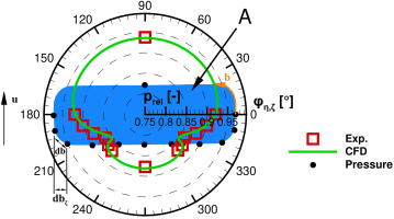
Integrating the wall pressure profile at the cross-section gives the load vector Ls,ξ (Equation 1). The load represents the aerodynamic lift exerted on the perimeter of the cross-section. More inhomogeneous flow will result in higher load and greater pressure losses, indicating that this is an appropriate parameter (Grois et al., 2023, 2024). The coefficient is calculated using the maximum load occurring in the duct flow.
The parameter for the distorted mass flow ratio μdi is defined by the separation of the sectional areas into clean (cl) and distorted (di) fractions (Equation 2) (Figure 5). The limiter for the splitting is the area averaged total pressure p¯t,Q at the cross-sections minus a half of the intake pressure loss Δpt,i. This approach has proven to be the most versatile. As a result, the parameter identifies changes in the flow behavior along the intake flow (μΥ,di) (Equation 2).
Figure 5.
Total pressure pt plot with clean (cl) and distorted (di) split (left) and advanced distortion descriptors SKE (middle) and ωsec (right) (area sectioning: SI - central flow separation (SB), SII and SIII - lateral vortices (LV)), (DOP).

The area integral of the secondary kinetic energy Secondary Kinetic Energy (SKE) (Equation 3) is based on the velocity components perpendicular to the main flow direction and aligned with the blue ξ,η,ζ coordinate system. Secondary flow occurs in regions where the forces acting on a fluid element tend to deflect that fluid element from the primary direction, which, in this case, is mostly aligned with the centerline of the duct. The generated vortex systems cause a partial transformation of kinetic energy into SKE (Nikitin et al., 2021). Therefore, the SKE indicates flow losses and identifies areas of flow interaction, e.g. between vortices (Figure 5). The coefficient cSKE,A is defined using (12ρv2)DIP at the DIP to show the rise with the duct flow.
The vorticity ω is a principal parameter obtained from the velocity field that indicates the presence of vortical structures. It uniquely identifies the dimensions of the vortex and its core. In addition, the secondary vorticity ωsec includes flow components that are perpendicular to the main flow direction and can be used as an additional indicator of longitudinal vortices (Equation 4). Positive and negative signs allow the differentiation of flow regions into right- and left-spinning parts, as shown in the colored Figure 5 (right). The classification by region (SI, SII, SIII) enables information to be obtained from certain phenomena that occur in the flow of the MEIRD. The coefficient cω,sec,A is formed by the vorticity magnitude along the duct flow to show the secondary part in relation.
The distortion coefficient DC60 (Equation 5) specifies the total pressure distortion for a certain cross-section in a fixed angular range of 60 degrees. This allows the intensity of the flow non-uniformity to be determined. The method is based on SAE standards and uses pressure transducers on the cross-section (SAE International, 2011, 2017).
The swirl coefficient SC60 (Equation 6) is defined by an analogous angular sector. It is determined by the ratio of the mean circumferential speed vφη′,ζ′,max,60 to the mean axial speed vQ. φ is the circumferential coordinate of the polar diagram of the cross-sections.
Unsteady post-processing
The post-processing is designed to determine advanced distortion coefficients to quantify the unsteady intake compressor interaction. Given the computing time required, the time-consuming CFD simulation and the resulting data are post-processed in parallel (Figure 6). The boundary conditions for the CFD are derived from the test bench conditions of the experiments used for the validation. The steady-state CFD serves as an initial solution for the transient simulation. Unsteady CFD results are exported for each third of a single LPC rotation. This corresponds to a time step of 1.464⋅10−3 s and a nominal sampling rate of 683 Hz for the parameter’s temporal signal capture. The maximum expected dominant intake flow frequency is fmax,intake=193 Hz, which was experimentally determined (Rademakers et al., 2024). Phenomena with frequencies up to the LPC rotation (flpc,N76=227 Hz) must be considered. One study also detected phenomena with a frequency range of 250–450 Hz in the center of the AIP (Tanguy et al., 2018). The Nyquist-Shannon theorem specifies a sampling rate twice that of the output signal to be fully determined (Granot, 2019). In post-processing step (1), the exported time step data are analyzed with pyTecplot. The distortion descriptors are calculated and recorded. The determined parameters are used to create contour plots of AIP and DOP. In the post-processing step (2), the specific distortion parameters are read in a temporal series. The data is analyzed for a limited time-period. Due to the small amount of temporal data available, the signal is resampled using the Fourier method (Laird et al., 2004). Dominant frequencies of the resulting temporal signal of each distortion parameter are quantified using Power Spectral Density (PSD) analysis. The estimation is based on the periodogram method, a function of the fast Fourier transformation. Studies have shown that URANS simulation with PSD analysis can provide results similar to experiments and scale-resolved simulation (Liu et al., 2024). Frequencies are given as the Strouhal number St (Equation 7), which is well suited for comparing the obtained results with data from the literature. Studies also showed that a simple bent pipe for analyzing transient flow phenomena is mostly at lower Reynolds numbers, below 106 (Rademakers et al., 2024), which can be transferred to the basic duct flow. Typically, the unsteadiness of secondary flow phenomena, such as shear layer instabilities, or vortex switching and local vortex shedding occurs between 0.1<St<0.4 (Rütten et al., 2005). Recent experimental studies by Garnier found dominant total pressure fluctuations (0.25≤St≤0.625) caused by secondary flows downstream of an s-duct (Garnier, 2015).
Figure 6.
Post-processing chain, unsteady intake and LPC interaction distortion descriptors analysis.

Results
General flow behavior
The analysis of the general flow behavior and the vortex systems helps to understand the aerodynamics of the intake system (Figure 7). The duct flow is characterized by two dominant phenomena: the lateral vortices LV and the large central flow separation SB, which are discussed in this paper and analyzed in terms of their frequency modes.
Figure 7.
Flow behavior and vortex systems of the MEIRD, cross-sections Qx with PR=pt/pt,DIP, Q-criterion, and radial iso-surfaces with colored TKE.
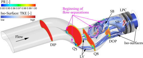
In the area near cross-section Q5, early flow separation occurs due to the inflow of low-energy fluid. This leads to the formation of the lateral vortex pair LV, which is caused by the thick boundary layer and the kidney-shaped inlet geometry. The flow, accelerated by the strong curvature near cross-section Q8, causes strong pressure gradients and a large central flow separation (SB). The intake design prevents further deceleration of the flow. The main distortion pattern is driven by the large central flow separation SB. At the DOP, different phenomena result in a highly interacting system, capturing diverse modal frequencies, as shown in the following unsteady analysis. Near region SB*, the SB expands and shapes around the spinner, following the direction of LPC’s rotation. A comprehensive flow analysis along with phenomenological descriptions can be found in the work of Hanrahan et al. (2025) and Grois et al. (2023, 2024).
Flow distortion pattern
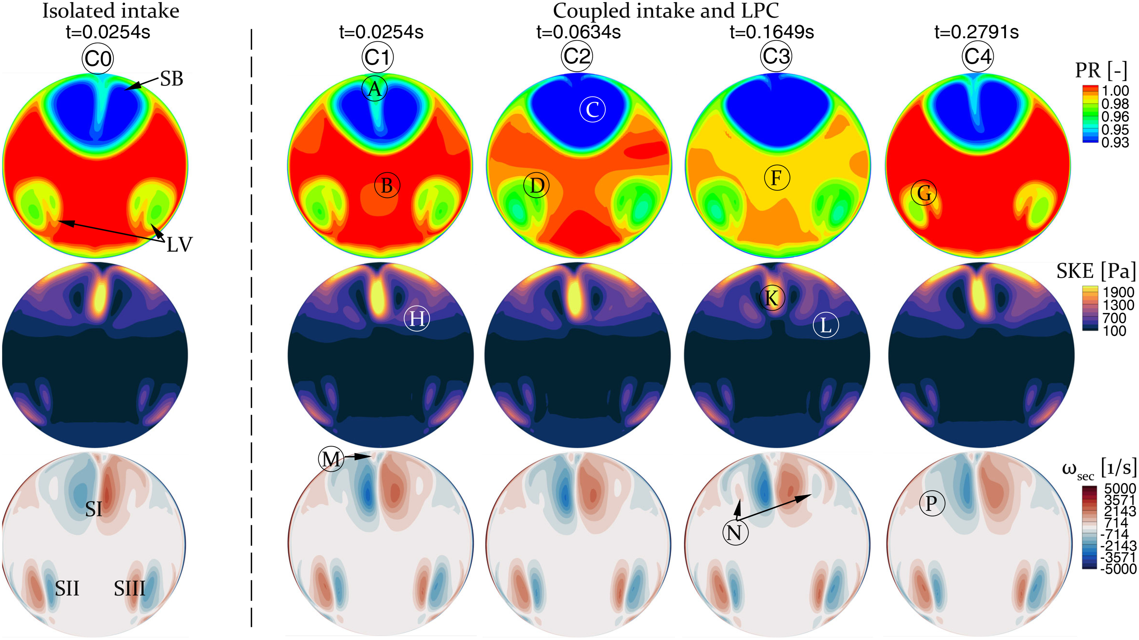
The flow distortions are classified by the different distortion descriptors at the DOP for specific time steps (Figure 8, Table 1). This allows certain states of flow distortion to be shown using descriptors with different sensitivities, which helps one to understand the later frequency analysis in this study. The time steps show key aspects of the periods with significant phenomena. The contour plots compare one time step for the isolated intake (left column,  ) with four time steps of the coupled intake and LPC configuration (right columns,
  ,
,  ,
,  ,
,  ). The later analysis will show that the vortex structures of the isolated intake change minimally over time (Section “Isolated intake”), meaning that only a single time step of the isolated intake is shown and used as a basis for comparison.
Figure 8.
Flow distortion pattern (PR (top), SKE (middle), ωsec (bottom)) at the DOP for different time steps, comparison of one time step of the isolated intake and four time steps of the coupled intake and LPC.
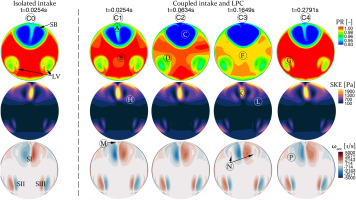
Table 1.
Flow distortion descriptors, discrete values for specific time steps and LPC revolutions, comparison of one time step of the isolated intake (Iso. int.) and four time steps of the coupled intake and LPC (Cpld.).
| | Iso. int. | Cpld. |
|---|
| t | [s] | 0.0254 | 0.0254 | 0.0634 | 0.1649 | 0.2791 |
|---|
| rev | [-] | (5.8) | 5.8 | 14.4 | 37.6 | 63.5 |
|---|
| cω,sec,A | [-] | 0.058 | 0.063 | 0.062 | 0.058 | 0.061 |
| cL,s,ξ | [-] | 0.089 | 0.080 | 0.078 | 0.073 | 0.076 |
| cSKE,A | [-] | 0.138 | 0.135 | 0.133 | 0.111 | 0.121 |
| μΥ,di | [-] | 0.276 | 0.274 | 0.257 | 0.185 | 0.315 |
| DC60 | [-] | 0.662 | 0.579 | 0.697 | 0.648 | 0.696 |
| SC60 | [-] | 0.259 | 0.277 | 0.255 | 0.263 | 0.254 |
The dominant flow phenomena LV and SB are displayed for isolated intake (). In the middle section of the SB, there is a peak in SKE, indicating strong interaction between the vortices (middle row). Regions SI, SII, and SIII show the clear split and position of the right- and left-turning flow components of the vortices (bottom row).
A comparison with the same time (t=0.0254 s, ) reveals a similar distortion pattern for the coupled intake and LPC configuration. The asymmetry Ⓐ points in the opposite direction (compared to ) toward the LPC rotation. In the center of the DOP Ⓑ, an upstream effect of the spinner caused by a local change in PR is observed. The SKE shows a local increase in region Ⓗ compared to the isolated intake. The central pair of small vortices above the SB (Ⓜ) shows a reverse direction of rotation compared to (ωsec colors switched). Therefore, the DC60 is 12.5% smaller at 0.579 (Table 1) compared to the isolated intake. The cSKE,A remains almost unchanged, which highlights the observations. cω,sec,A increases from 0.058 to 0.063.
As time progresses (t=0.0634 s, ), a change in total pressure distortion pattern emerges. The SB is becoming larger (Ⓒ). The LV’s area of influence is larger, so the region with lower PR is wider Ⓒ. A change in the distribution of SKE and ωsec at the DOP is minor for compared to . The discrete values for t=0.0634 s show, only an increase in DC60 compared to t=0.0254 s (Table 1). This is due to the 60∘ weighted section, which detects the increase due to the local PR drop of the SB.
At t=0.1649 s (), no further change in the SB can be observed in means of the PR distribution. A global drop in PR occurs in regions around the vortices at the DOP (Ⓕ, orange contours). The region of interaction of the SB vortex cores is smaller in terms of SKE (Ⓚ). In area Ⓛ, in the middle of the left and right vortex cores of the SB, a local rise in the SKE forms, indicating a splitting of these cores. The ωsec shows this splitting phenomenon with two additional counter-rotating pairs of vortices Ⓝ. In terms of the discrete values, the reduction in SKE at interaction region Ⓚ leads to a significantly lower cSKE,A of 0.111 compared to the other time steps (Table 1). The ratio of distorted mass flow μΥ,di decreased by 32% compared to , indicating a substantial reduction in flow non-uniformity.
The distortion pattern at resembles that of , with 16.8% variation in DC60, and similar flow topology. The drop in PR is limited to the regions of the SB and the LV. However, the LV’s area of influence is smaller (Ⓖ). The SB shows a clear and closed shape (Ⓟ), with no signs of splitting. The ratio of distorted mass flow μΥ,di is highest at 0.315 compared to the other time steps (Table 1).
Isolated intake
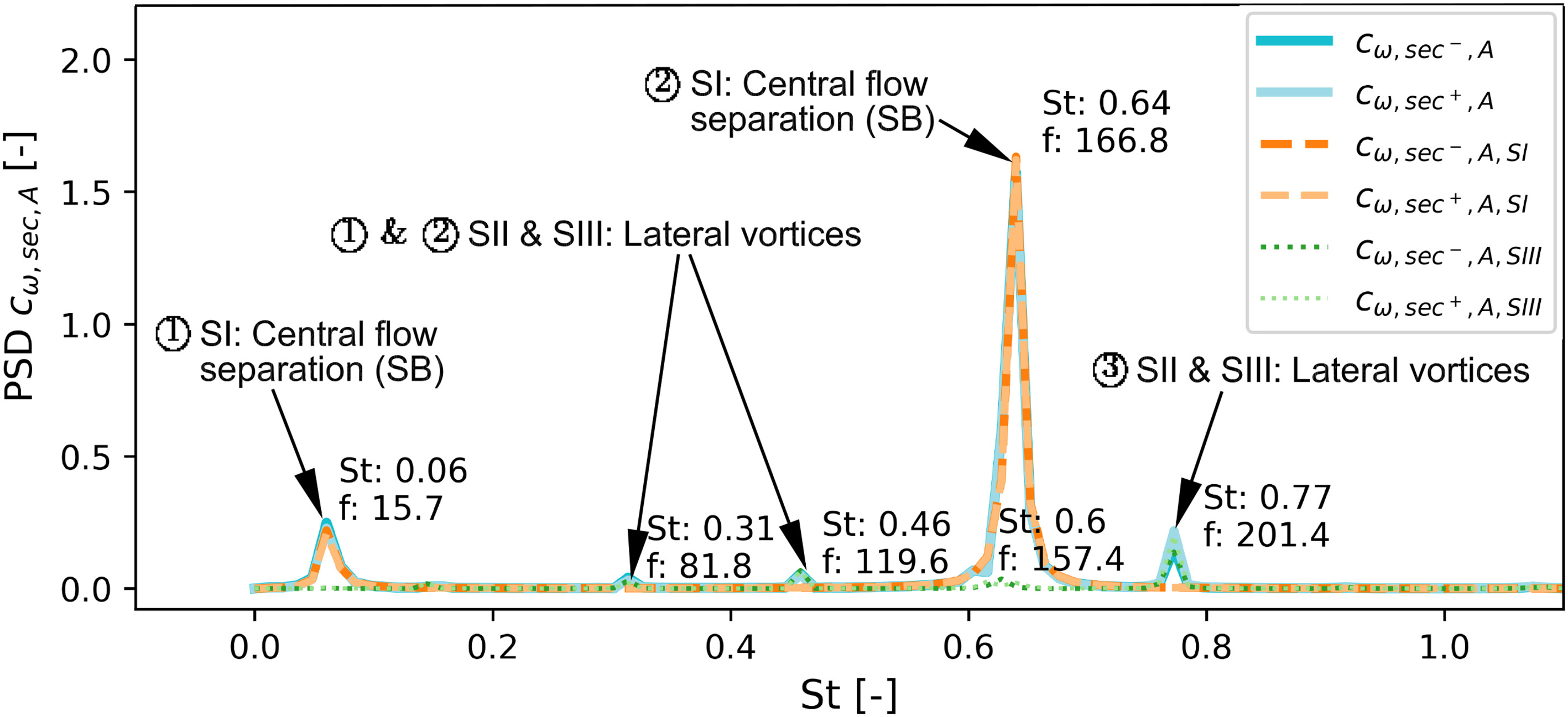
The frequency analysis of the isolated intake enables the identification of isolated flow phenomena. The analysis of the temporal signal characteristics of the flow distortion parameters refers to the DOP. The influences of the compressor are excluded. The vorticity ω is a quantity related to rotation of the velocity field of the flow in the duct, and is highly sensitive to the dominant frequencies of mainly longitudinal vortex systems. Figure 9 shows the PSD analysis of cω,sec,A, divided into the three sub-regions SI, SII, and SIII, and into the right (+) and left-spinning (−) parts of the flow. The sub-areas are assigned to the locally occurring flow phenomena: lateral vortices (LV) and the large central flow separation (SB). In this way, the PSD analysis enables the division of the various modal frequencies (➀, ➁, and ➂) of the respective phenomena. The blue lines show the entire cross-section without subdivision, for the right (+) and left-spinning (−) flow parts.
Figure 9.
Spectral analysis of the subdivided flow distortion descriptor cω,sec,A, colored lines for right and left spinning flow parts, isolated intake, f in [Hz].
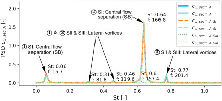
The central flow separation shows two dominant frequencies; ➀: St=0.06 at 15.7 Hz and ➁: St=0.64 at 166.8 Hz. These can be assigned to this flow phenomenon since only a trigger in the SI area occurs (region of the central flow separation). Three further modes are caused by the lateral vortex systems in the SII and SIII regions; ➀: St: 0.31 at 81.8 Hz, ➁: St=0.47 at 119.6 Hz, and ➂: St=0.60 at 157.4 Hz. For small Stouhal numbers (St<0.1, ➀ SB), the flow remains relatively steady. The low frequencies are associated with large-scale instabilities and are independent of the Reynolds number for an ideal and limited case of a sphere (Kim and Durbin, 1988). At higher Strouhal numbers (St>0.3, ➁ SB, ➀ ➁ ➂ LV), strong periodic vortex shedding leads to high-pressure oscillations (Silva-Leon and Cioncolini, 2019). The higher Strouhal numbers are caused by small-scale instabilities from the separation of the shear layer (Sakamoto and Haniu, 1990). This increases the risk of strong flow separation, which can potentially cause an LPC stall event. It also produces aerodynamic noise and structural vibrations in the intake duct (Xiong et al., 2019). Significant total pressure distortion at the front of the engine results in reduced engine performance. If the intake’s resonance frequency matches the separation frequency, resonant amplification can occur, leading to structural damage.
Clockwise and counterclockwise flow components do not differ in their frequencies. The lateral vortex systems’ right (SIII) and left (SII) sides show the same modes, so only SIII is demonstrated (Figure 9). In the experimental investigation by (Rademakers et al., 2024), the most dominant frequency of also 153 Hz was recorded by four high-frequency pressure transducers mounted at different positions along the intake wall, which shows the global dominance of the associated flow phenomenon. The closest numerical frequencies are at f=157 Hz, but these are slightly induced by the lateral vortices. The frequency of 166.8 Hz (➁ SB), which clearly dominates in the numerical results, corresponds more closely to the observations from the experiments, but is slightly shifted. However, since the influence of the LPC is absent, deviating frequencies are assumed. The third mode of the lateral vortex system is also observed in the experiment (at 193 Hz, nred,rel=76%) and is significantly less prominent than the mode at 153 Hz. Further frequencies are found in the range of 100 Hz, which are identified as stronger within the aft end of the duct. This corresponds to the spectral range of the first and second modes of the lateral vortex system. Previous studies have shown that these vortices interact strongly and exhibit small-scale fluctuations that URANS simulations cannot completely cover. Since the primary modes can also be detected in the isolated intake simulation, it proves the statement of Rademakers et al. (2024) that the three modes are independent of LPC rotational frequency and are mainly induced by the geometry of the intake.
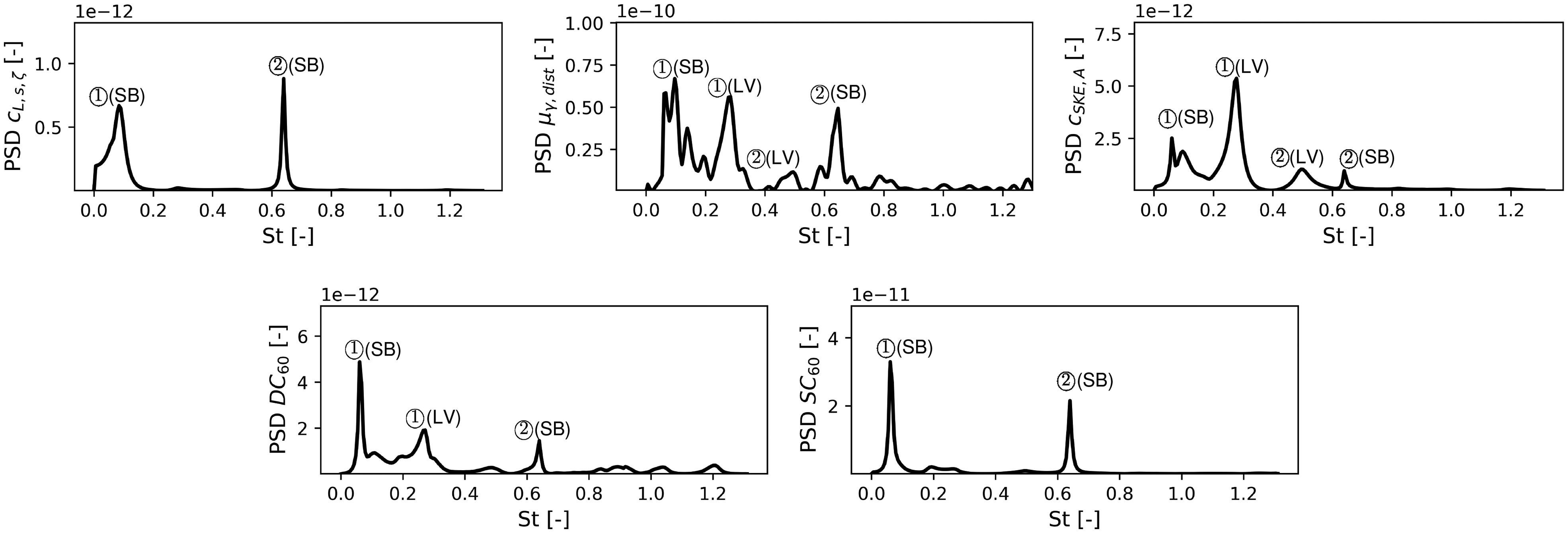
The load coefficient cL,s,ξ is a way of measuring the flow’s inhomogeneity and the intake wall’s structural load. Figure 10 (left, top) shows the PSD analysis corresponding to cL,s,ξ. No subdivision into different sections has been made. The two dominant frequencies of the central flow separation (SB) can be seen. The lateral vortex systems do not affect the temporal signal of the load. Consequently, the structural impact of the SB is expected to be the major one.
Figure 10.
Spectral analysis of the distortion descriptors cL,s,ξ (left, top), μΥ,dist (middle top), cSKE (right top), DC60 (left bottom), SC60 (right bottom), isolated intake.
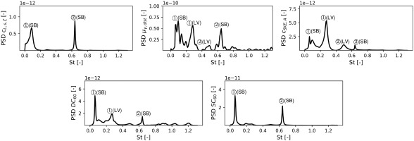
The μΥ,dist is highly suitable as an input for low-fidelity simulations due to the division of the flow into distorted and clean (Remiger et al., 2024). Figure 10 (middle, top) shows a volatile curve of the PSD analysis, which impedes the explicit identification of dominant frequencies. The first two frequencies of the central flow separation (SB) and lateral vortex systems (LV) are shown. The impact of ➀ (LV) is higher than the previous flow distortion descriptors.
The corresponding analysis of cSKE shows similar results (Figure 10, right, top)). The first two dominant frequencies of the flow phenomena can be identified, with ➀ (LV) being indicated as the most dominant. The temporal effects of the transformation of kinetic energy into SKE through the vortex systems are strong here.
The DC60 enables the detection of the first two modes of the SB and the first mode of the LV. The most dominant is the ➀ (SB). With lower Stouhal numbers, there are less strong temporal effects on the flow inhomogeneity (St<0.1). This limits the usability of the DC60 as a dynamic flow distortion descriptor.
The SC60 shows similar behavior. In this case, it only detects the SB phenomena. Temporal swirl fluctuations caused by less dominant vortex systems (LV) are neglected.
A different sensitivity can be observed by comparing these flow distortion parameters for the steady-state CFD and the unsteady behavior of the URANS simulation. The steady-state load value cL,s,ξ is close to 0 at the DOP. This is known from previous studies (Grois et al., 2023). Here, the cross-sectional load was mainly influenced by the geometric shape of the intake, which passes zero at the outlet. Consequently, the load on the DOP is roughly steady. The evaluation of the URANS shows a deviation margin of <0.1%. The stationary value of μΥ,dist reaches 34.6%. The temporal signal has a span of 0.39% over minimum and maximum. The impact of the change over time is minor. The stationary cSKE reaches 0.138 at the DOP. Over time, a maximum drift of 0.15% can be seen. cω,sec,A is defined as the ratio relative to the maximum vorticity occurring in the intake. With the DOP as a reference, a stationary value of 5.8% is obtained. As with the load, the fluctuation of the secondary vorticity is less than 0.1%. The DC60 achieves a value of 0.662 when the results of the steady-state CFD are considered. The deviation is minor with <0.1%. The stationary SC60 is 0.259. The time-related deviation is 0.12%.
Coupled intake and LPC
The coupled simulation results include the intake and the two-stage-LPC with spinner. The coupled approach allows conclusions to be drawn about the direct influence of the LPC on the intake flow behavior. The correlation between the Stouhal number and the frequency differs from the isolated intake observation since a slight change in the intake operating point occurs due to the coupling of the LPC. This temporal analysis of the flow distortion parameters refers to DOP.
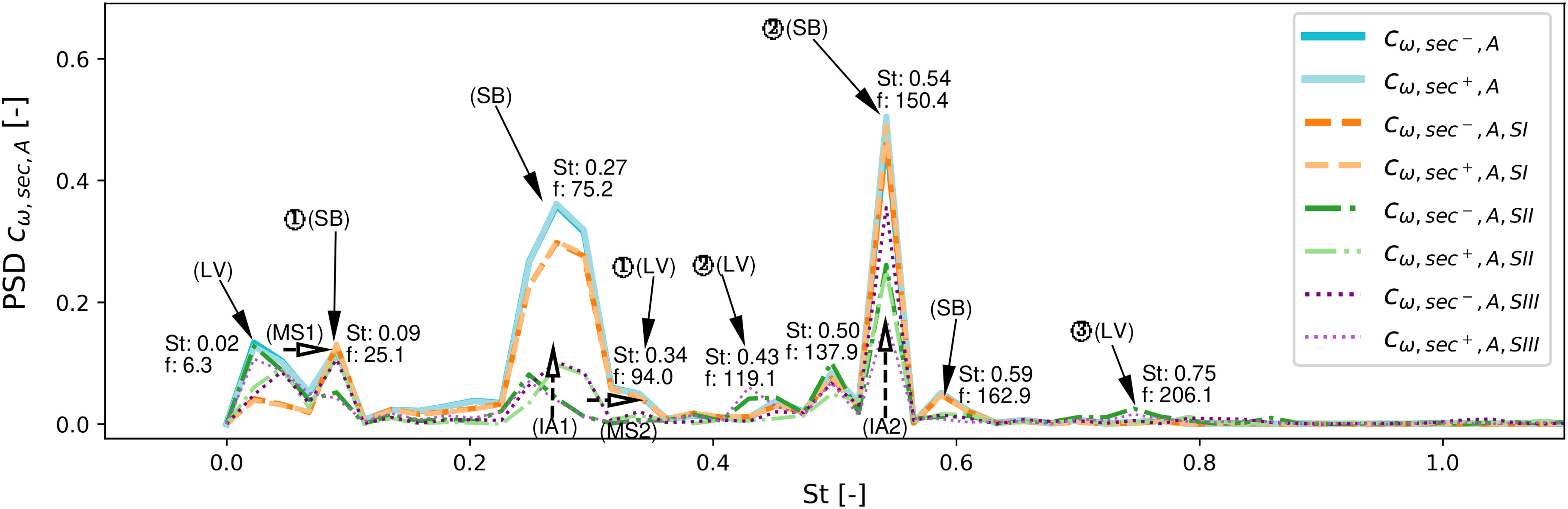
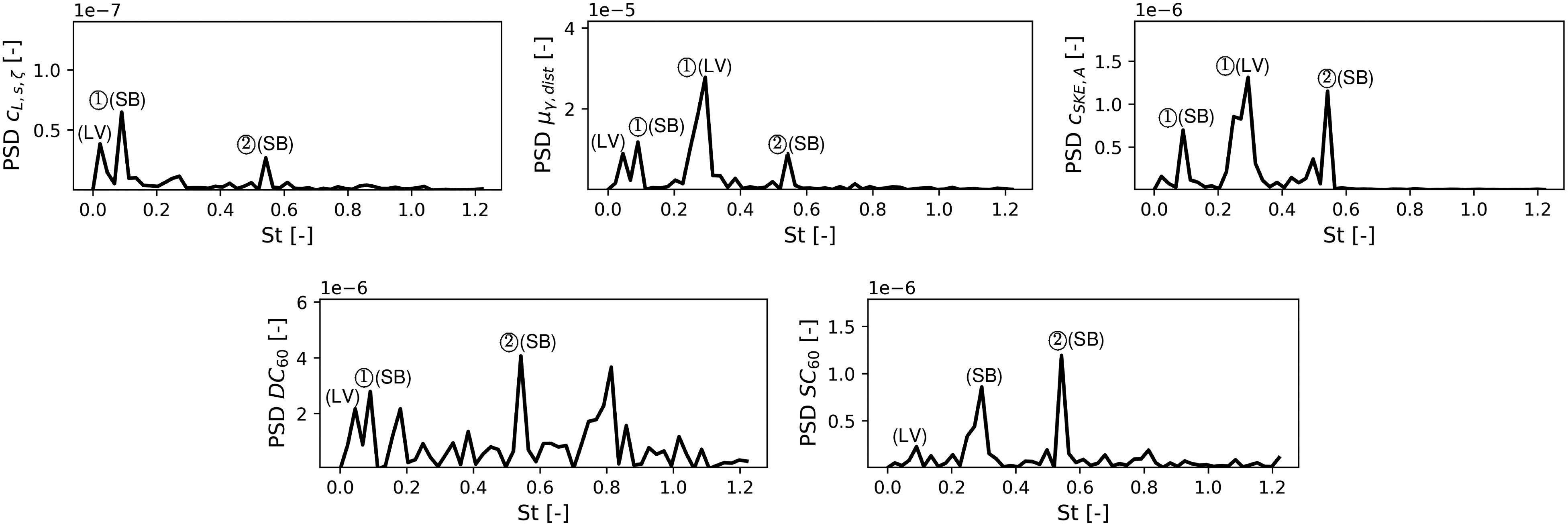
The differences between the coupled and the isolated simulation results are evident when comparing the dominant frequencies of cω,sec,A (Figure 11). The first modal frequency of the large central flow separation (SB) was shifted (Modal Shift (MS) 1) from f=15.7 Hz to f=25.1 Hz. An additional low-frequency (St=0.02, f=6.3 Hz), which can be assigned to the lateral vortex system (SII and SIII), emerged. At f=75.2 Hz, an additional dominant frequency of SB appears, which was not present in the isolated intake analysis. The large-scale domination leads to the lateral vortex system’s Induced Amplification (IA) 1. The previously identified first and second modes of the lateral vortex system in the isolated intake can also be found. ➀ (LV) is shifted from f=81.8 Hz to f=94.0 Hz (MS2). The experimental results of (Rademakers et al., 2024) show in these spectral ranges (103Hz<f<108 Hz) also a second dominant frequency, which can be assigned to the interaction of the SB (at 75.2 Hz) and LV (➀: St: 0.34 at 94.0 Hz and ➁: St: 0.43 at 119.1 Hz). The most dominant frequency (➁ (SB)) matches the value from the experiment, with f=150.4 Hz of the URANS results and f=153 Hz in the experiment. This modal frequency is again found to be the most dominant in CFD and experiment. The mode can be assigned to SB, but its intensity stimulates the lateral vortex system (IA2). This dominant distortion frequency corresponds to approximately 0.66 times the LPC rotational frequency (227 Hz at N76). The third mode, known from the experiments (Rademakers et al., 2024), can only be detected in its beginnings (➂ (LV)). The frequency from the CFD at f=206.1 Hz is close to the experimental value at f=193 Hz. The overall time series of cω,sec,A for the coupled simulation shows a more diffuse behavior of the individual parameters (SI, SII, SIII) for identifying the vortices and flow separations. The detected frequencies of the right- and left-spinning flow components for the LV system only do not always match exactly (+, −), especially in the range of the induced frequency (IA1). Additional dominant frequencies have emerged and are stimulating adjoining vortex systems. A complex interplay between the diverse vortex systems’ interaction and the LPC’s upstream effect is evident. An excitation directly associated with the rotational frequency of the LPC was not found by the signal of cω,sec,A. The temporal cL,s,ξ analysis shows minor differences when comparing the isolated intake results and the coupled results (Figure 12, left, top). The low frequency (St=0.02, f=6.3 Hz) additionally found in Figure 11 is also detected by the load coefficient. This underscores the coupling of the LPC as a trigger. μΥ,dist clarifies the modes found in the isolated intake. ➀ (SB) is less dominant. The cSKE signal shows ➁ (SB) more dominant than in the isolated intake case. This indicates that the secondary flow losses in the central flow separation (SB) region increase due to the coupling of intake and LPC. The time-resolved DC60 shows a more discontinuous curve with less distinct dominant frequencies. A peak in the range of St=0.8 appears, which was not found by any other parameter. Analogous to the previous parameters, the SC60 also shows an additional mode at St=0.27, which only occurs in the coupled case.
Figure 11.
Spectral analysis of the flow distortion descriptor cω,sec,A, subdivided regions, colored lines for right- and left-spinning flow parts, coupled intake and LPC, f in [Hz].
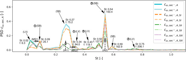
Figure 12.
Spectral analysis of the distortion descriptors cL,s,ξ (left, top), μΥ,dist (middle top), cSKE (right top), DC60 (left bottom), SC60 (right bottom), coupled intake and LPC.
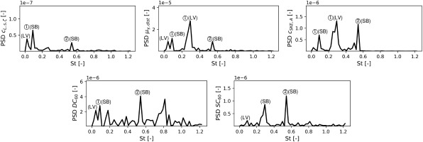
The steady-state values of the flow distortion descriptors differ only slightly between the isolated intake and the coupled case. cL,s,ξ is also close to 0 at the DOP. The distorted mass flow ratio μΥ,dist is slightly lower at 27.3% for the coupled results compared to the isolated ones. The coefficient of the secondary vortex cSKE is 0.06, which is also less than the value from the isolated CFD. With 6%, cω,sec,A is slightly higher compared to the isolated intake value. The DC60, with 0.660, does not differ. The SC60 is marginally larger at 0.264.
An evaluation of the deviations of the minimum and maximum values of the time signal shows more significant differences than the isolated intake results. The load showed an almost stationary behavior in the isolated intake analysis. The coupled investigation revealed deviations over time of 8.5%. The amplitudes of the μΥ,dist signal have a spread of more than 63% in the coupled simulation. This shows that this parameter captures the LPC’s upstream effect particularly sensitively. Also, cSKE with 36.4% signal spread reacts strongly to LPC influences. This is due to the increase in secondary flow losses caused by the superimposition of rotation on the flow through the LPC. The DC60 varies by 20.3% and reaches a maximum of 0.71. This corresponds to a very high value, which indicates a (temporary) strong total pressure distortion. Since a steady-state value usually serves as a basis for the design of the intake and engine, this illustrates the importance of analyzing unsteady fluctuations. The SC60 fluctuates insignificantly by 14.7% over time.
Influence of the axial position
Previous studies showed a major influence of the axial distance of the engine to the duct’s aft end on the flow distortion behavior (Rademakers et al., 2024). This work analyzes two interfaces between the intake and the engine. The DOP is located directly at the outlet of the duct. The AIP is located 0.48⋅dDOP downstream of the DOP. This corresponds to a realistic distance in real applications. Studies have shown that the flow is already mixing between DOP and AIP, and the flow inhomogeneities are decreasing. The various flow distortion descriptors showed different behavior when the flow was mixed (Grois et al., 2023). In the following, the results of the coupled simulation are analyzed.
The time-averaged DC60 decreases by 18.9% downstream to the AIP. Since the spinner position is close to the AIP, an upstream effect of the spinner nose can already be observed. This leads to displacing the surrounding vortices and flow separation areas from the incoming flow. This displacement effect has a negative impact on the detection of a 60∘ sector by the DC60, so that a strong drop occurs. cL,s,ξ is close to 0 at the DOP and causes a change in sign at the AIP. The surface load on the outlet channel downstream the duct can increase more than necessary if the positioning is unfavorable in aircraft design processes. On the other hand, the secondary flow losses detected by the SKE (CSKE,A) decrease by 24.0%, which can positively affect the flow to the LPC blades. The ratio of the distorted mass-flow μΥ,dist increases by 22.4%, which has also been shown in studies (Grois et al., 2023). Like the DC60, the flow distortion is described by an angular section with a drop in total pressure across the interface. This is related to the description of the distorted mass flow μΥ,dist. However, an opposite behavior is observed here. In other words, various flow distortion descriptors must be used in the design process to consider an appropriate axial position in combination with the proper engine characteristics.
Conclusion
A highly bent engine intake’s flow is characterized by specific frequencies, spatial structures, and dynamic phenomena, which can be clearly identified and quantified by an unsteady analysis and advanced flow distortion descriptors. This knowledge enables a direct causal link between intake flow distortions and their impact on engine performance and vice versa. As a result, weaknesses in intake design can be systematically identified and addressed through targeted geometric modifications or flow control strategies. This study systematically investigates advanced flow distortion descriptors to quantify unsteady intake flow phenomena and their interaction with the LPC.
The analysis of the isolated intake revealed two dominant unsteady flow phenomena
Lateral vortex systems (LV) in the side regions (SII, SIII) exhibit three dominant modal frequencies at 81.8, 119.6, and 157.4 Hz, corresponding to 0.31<St<0.60.
The load coefficient cL,s,ξ primarily captured the impact of the central flow separation (SB), indicating its significant structural relevance. Other descriptors like distorted mass flow ratio μΥ,dist and coefficient of the secondary kinetic energy cSKE,A additionally reflected the dynamic behavior of lateral vortices.
Classical descriptors such as DC60 and SC60 were less sensitive to higher frequency, small-scale vortex dynamics, confirming the added value of the advanced parameters introduced.
The CFD results and the experiment data agree well. Strong flow separation will reduce the model’s accuracy.
A frequency shift of the large central flow separation’s (SB) first modal frequency from 15.7 to 25.1 Hz and the emergence of a new low-frequency mode at 6.3 Hz related to the lateral vortices is caused by the LPC coupling.
A new dominant SB mode at 75.2 Hz, not observed in the isolated intake, indicating an induced amplification of lateral vortex systems through LPC interaction is found.
The most dominant frequency of the SB at 150.4 Hz was confirmed and matches experimental observations, highlighting the robustness of the numerical approach.
At certain periods (e.g., t=0.1649 s), the vortex cores of SB split, which is indicated by a drop in cSKE,A and the distorted mass flow ratio (μΥ,di).
Across all parameters, the temporal variations remained small relative to the mean values, but the frequency content analysis highlighted that specific modes can strongly affect flow inhomogeneity and potential engine performance risks. A complete spectrum of the dominant frequencies of aerodynamic phenomena could not be found without coupling the LPC. The parameters for quantifying flow distortion are variable over a period of time. Potential maximum values would be ignored in a steady-state analysis and could affect engine performance.
Given the flow field at the intake outlet, the specific frequency, location and phenomenon can be precisely determined. By understanding which frequencies and locations in the intake flow negatively affect engine performance, the intake geometry can be systematically optimized to avoid or mitigate these effects. By adjusting the intake design, weaknesses in the system can be specifically addressed and the performance of the engine can be improved.




 ) with four time steps of the coupled intake and LPC configuration (right columns,
  ,
,  ,
,  ,
,  ). The later analysis will show that the vortex structures of the isolated intake change minimally over time (Section “Isolated intake”), meaning that only a single time step of the isolated intake is shown and used as a basis for comparison.