Introduction

Machine learning (ML) methods have gained significant popularity for their ability to integrate statistical knowledge with physical equations and constraints, leading to more robust and interpretable models (Yue et al., 2022; Senior and Miller, 2024; Zhang et al., 2024). When focusing on ML methods, it is evident that data, as the foundation of the model, plays a critical role, with its quality and balance often becoming the limiting factors in industrial applications. In existing surrogate model research within the field of compressor aerodynamics, dataset construction primarily follows two approaches. The first is purely mathematical Design of Experiments (DOE) methods, such as Central Composite Design (Angelini et al., 2020) and Bayesian Optimization (Senior and Miller, 2024). The second approach leverages the blade design of typical fans/compressors (Zhang et al., 2024). To ensure the generalization capability of ML, the parameter range of the dataset is typically broad. However, for compressor flow fields, extreme values of aerodynamic parameters can lead to issues such as difficulty in achieving computational convergence and the occurrence of severe flow separations, resulting in flow fields that are practically unusable. Given the limited practical combinations of airfoil shapes and flow conditions, purely mathematical DOE methods frequently generate impractical samples (Schmitz et al., 2011). Conversely, sample generation methods based entirely on historical airfoil designs tend to concentrate geometric and aerodynamic parameters within a limited range due to their corresponding performance achievements, thereby introducing distribution bias in the modeling process. Domain knowledge, such as aerodynamic design rules (Senior and Miller, 2024) and choke Mach number (Yue et al., 2022), is used to constrain the dataset to physically realizable designs during preprocessing, i.e. after data acquisition. For datasets covering a wide parameter range, many samples are filtered out during data preprocessing. For instance, Yue et al. (2022) eliminated one-fifth of the original dataset during cleaning. If it is possible to determine in advance whether the flow field meets the dataset standards, significant computational costs and resources can be saved.

When applying domain knowledge in compressor aerodynamics, it is obvious that in compressor aerodynamics, severe flow separation represents the physical limits of the dataset. Following this line of thought, the problem of sample selection is transformed into a flow field classification problem. As Cumpsty (1989) addressed, the most important development in assessing the loading of cascades is attributable to the diffusion factor (DF) (Lieblein, 1953). For modern low aspect ratio, high-load designs, Lei et al. (2008) proposed a new judgment parameter, the stall indicator (SL), based on three-dimensional open corner separation. They also derived the diffusion parameter (DL) from design criteria. Later, Yu and Liu (2010) revised the calculation method for DL to obtain a modified diffusion parameter (DM) by incorporating the influence of aspect ratio, which improved the classification accuracy. Building on Lei’s research, Zhou et al. (2023) included axial force and derived the blade force spanwise decay parameter, SF, as well as the secondary flow intensity parameter (SI), which characterizes secondary flow through loss. The SI parameter exhibits a strong linear relationship with SF, enabling the classification of flow fields into three categories: two-dimensional separation, three-dimensional open corner separation, and no obvious separation. Since SI can be obtained by polynomial fitting of the design parameters, it provides a rapid assessment of whether the designed cascade meets the criteria from the perspective of loss, in contrast to the D factor, which is based on the limit load perspective.

For high-load designs with three-dimensional open corner separation, the SL and SF parameter can provide relatively accurate predictions. However, both of them require the integration of passage static pressure differences obtained through measurements or numerical simulations, making them unsuitable for direct application during the design phase. Parameters that can directly assist in design include DF, based on two-dimensional elemental flow, as well as its modified versions DL and DM, and the SI parameter, which is based on loss evaluation. However, all three judgment parameters have accuracy issues. Classifications based on DL and DM exhibit overlapping regions (Lei et al., 2008; Yu and Liu, 2010). The accuracy of SI in predicting three-dimensional open corner separation is compromised due to two reasons: First, when the aspect ratio is large, the proportion of secondary flow loss to the average loss decreases. In such cases, even if three-dimensional open corner separation occurs, SI remains within the range of 1.1 to 1.4, leading to misclassification of samples as having no obvious separation. Second, when severe three-dimensional open corner separation occurs, the loss at the mid-span also increase, causing SI to decrease.

In this paper, a supervised learning algorithm was chosen directly to address the flow field classification problem. The primary goal is to extend the application scenario of the classification model to the database construction phase. Based on Zhou et al. (2023)’s research, this study assigns flow field classification labels to the dataset. After analyzing and selecting the input features, the SVC algorithm, is applied to train the model. Ultimately, a data-driven classification model is developed that can evaluate flow in stator cascades during the preliminary design process by filtering out flow fields with severe separation, thereby achieving the goal of saving computational resources.

Methodology

The revised dataset design strategy is presented in Figure 1. As depicted in Figure 1a, the general approach for data cleaning using domain knowledge is typically applied during data preprocessing. In contrast, the revised approach proposed in this paper directly operates at data generation. The detailed process of integrating the revised approach into the dataset construction phase is illustrated in Figure 1b. The flow field classification model can be integrated with various DOE methods to generate blade geometries, ensuring a broad range of geometric parameters while avoiding severe separation. Furthermore, it directly defines the effective operating range, suggesting its utility not only for dataset generation but also for preliminary design of blade profiles.

Figure 1.

Revised dataset design strategy. (a) Revised application scenario for flow field classification and (b) Detailed process of generating samples in the dataset.

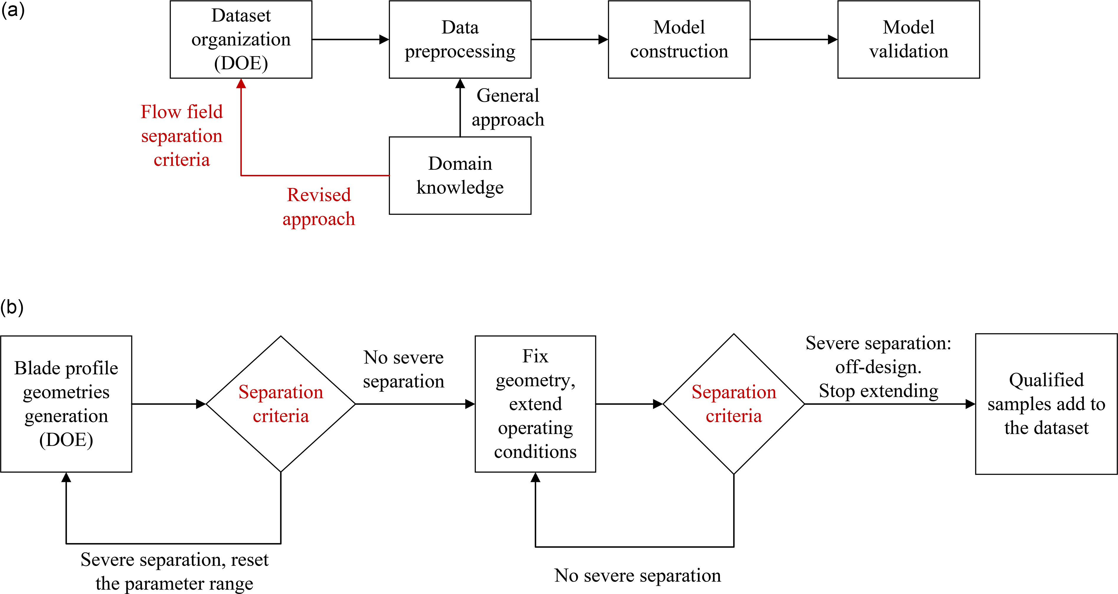
Based on the updates to the application scenario, the model establishment must meet specific requirements. In particular, all input features must be design parameters that can be obtained prior to the flow field computation. Second, determining separation criteria based on absolute values using a single empirical parameter is insufficient. Therefore, this study manually labels all samples in the dataset and trains a classification model. Building on the two points discussed above, this section will elaborate on the dataset organization and the flow fields labeling.

Dataset organization

The establishment of flow field classification criteria is based on the available data samples. In this study, a stator linear cascade dataset containing 889 numerical samples was used to train the flow field classification model. The 20 cascades of the database include cross-sections from the E3 HPC (Holloway et al., 1982) and the first three stages of a 9.271-pressure-ratio compressor (Steinke, 1986). Table 1 shows the parameter distribution, with further details in Yue et al. (2022) and Zhou et al. (2023). Flow field analysis and loss modeling based on this dataset have yielded promising results, proving the dataset’s reliability. As summarized in Table 1, the parameter range of the dataset broadly covers common stator airfoil designs. The present study specifically establishes flow separation-based criteria to further determine valid parameter ranges. All cases in the dataset exceed the critical Reynolds number, thereby excluding low-Reynolds number effects from the present investigation.

Table 1.

The parameter range of axial compressor stator cascade dataset.

Airfoil	CDA
Aspect Ratio	1.0 to 2.0
Inlet Metal Angle	38∘ to 58∘
Outlet Metal Angle	−6∘ to 22∘
Camber Angle	23∘ to 58∘
Chord	0.05 to 0.10 m
Pitch	0.03 to 0.09 m
Maximum Blade Thickness (over chord)	0.05 to 0.12
Passage Contraction Ratio	1.0 to 1.1
Incidence	−9∘ to +9∘
Inlet Mach Number	0.30 to 1.22

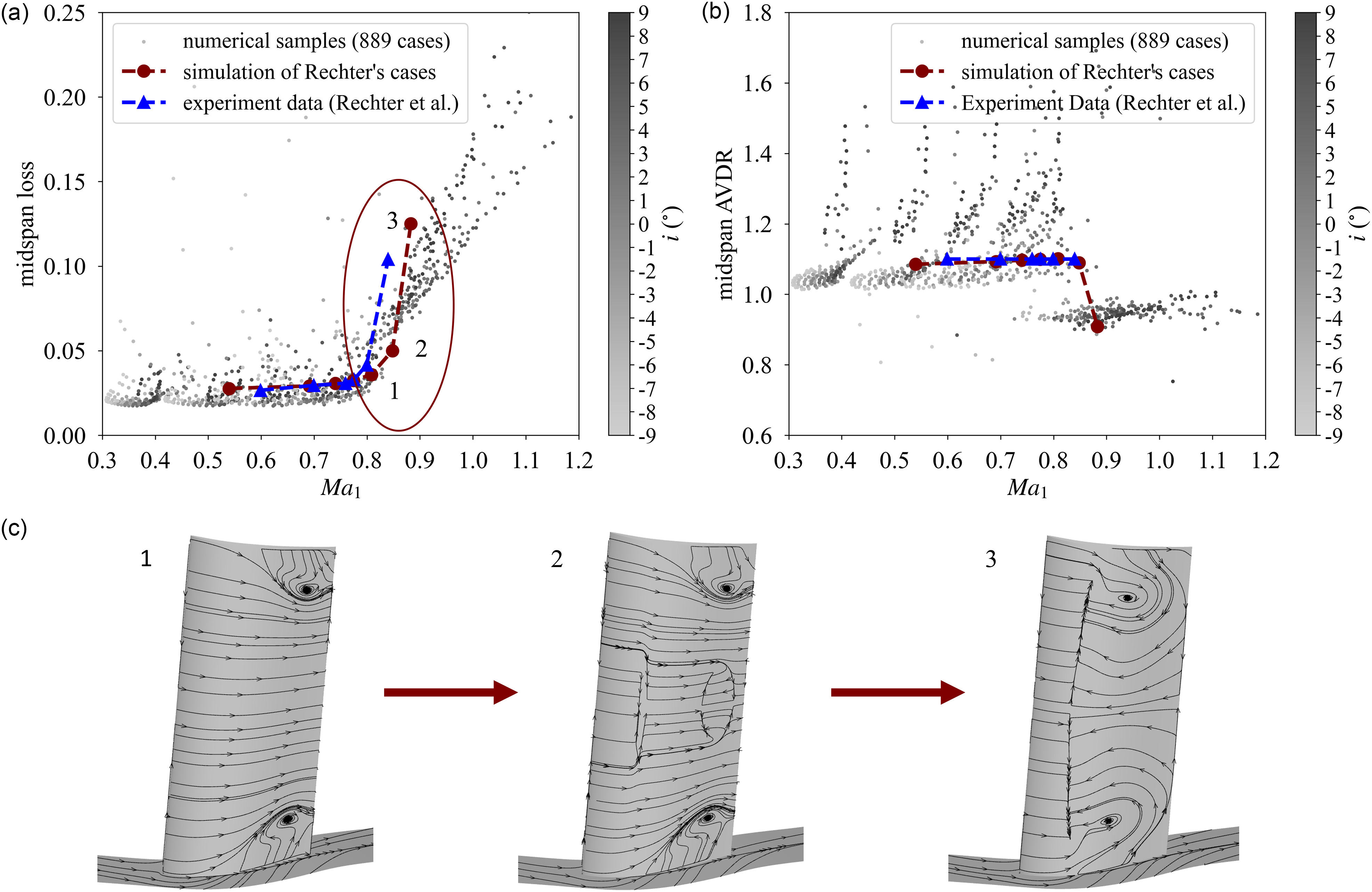
All 889 numerical samples in the dataset were generated using a consistent numerical framework: the Reynolds-averaged Navier-Stokes equations (RANS) method was adopted to generate simulations, and the Spalart-Allmaras (SA) turbulence model was chosen. The NUMECA v9.0–3 was the flow solver. Identical boundary conditions were applied across all simulations. Total pressure, total temperature and inlet flow angle were cast at the inlet and pressure was set at the outlet to alter the back pressure. All samples in the dataset were simulated using the same grid, which underwent a grid independence check and consists of 1.24 million nodes (Zhou et al., 2023). Figure 2a and b present a comparison between the numerical method used in this study and experimental results (Rechter et al., 1985), as well as the overall distribution of midspan loss and AVDR in the dataset. Combined with Figure 2c, it can be observed that the numerical results agree well with the experimental data near the design condition, where no significant flow separation occurs. However, when the inlet Mach number exceeds 0.8, reversed flow appears in the midspan region, leading to an underestimation of midspan loss in the numerical calculations. The accuracy of RANS models deteriorates under off-design conditions. From the perspective of dataset generation, this implies that an unrealistic parameter range can cause the flow fields to either fail to converge or exhibit severe separation. As a result, a large number of unreliable results are removed during data preprocessing, leading to a significant waste of computational resources. Figure 2c also reveals that fully spanwise 2D separation leads to a sharp loss increase, offering a basis for flow classification labeling.

Figure 2.

Comparison of numerical and experimental data (Rechter et al., 1985): (a) Midspan loss distribution across inlet Mach numbers, (b) Midspan AVDR distribution across inlet Mach numbers, and (c) Flow field topology variation for the inlet Mach numbers above 0.8 in deviated cases.

Labeling flow fields

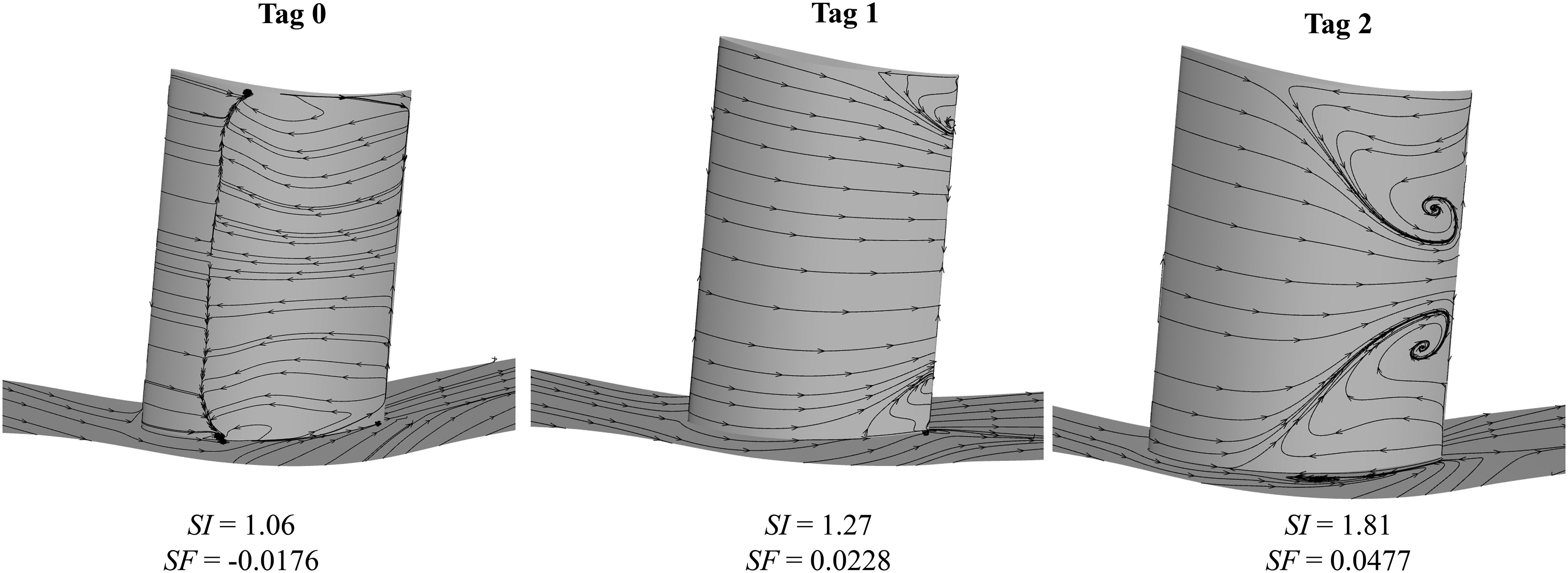
Following the computation of flow field information for all samples in the dataset, the subsequent step involves manually assigning tags to the three types of flow fields. Incorporating domain knowledge during labeling ensures the reliability and physical interpretability of the classification algorithm. For the three types of flow fields in the dataset, corresponding labels are assigned as follows: two-dimensional separation is labeled as 0, no obvious separation is labeled as 1, and three-dimensional open corner separation is labeled as 2. Figure 3 presents typical flow topology structures for the three types of tags. For two-dimensional separation, labeled as tag 0, the classification takes into account both the flow field topology (Taylor, 2019) and the incidence characteristics (Cumpsty, 1989). In the case of three-dimensional open corner separation, labeled as tag 2, the classification is determined by the presence of a ring vortex structure formed between the endwall and the suction surface (Schulz et al., 1989).

Figure 3.

Typical flow topology structures for the three types of tags.

Exploratory data analysis

Prior to model construction, dataset features were analyzed relative to the three tags. Statistical analysis of distribution patterns not only facilitates the understanding of different flow field structures but also offers valuable insights for the input features selection. Exploratory data analysis (EDA) was performed to visualize relationships between variables and select input features. Several aforementioned important dimensionless parameters, SF(1), DF(2), DL(3), SI(4) and AVDR(5), were used to describe the flow fields of different separation types. First, SF is a blade force spanwise decay parameter proposed by Zhou et al. (2023), similar to the stall indicator SL defined by Lei et al. (2008). SF reflects the deterioration of severe separation on the flow field through the spanwise difference of the blade force. SF is defined as:

Where fB represents the inviscid blade force. DF is the diffusion factor of Lieblein (1953). A DF exceeding 0.6 signifies a steep rise in wake momentum thickness, thereby serving as a critical indicator to characterize the two-dimensional diffusion limit (Cumpsty, 1989). DF is defined as:

DL is the diffusion parameter of Lei et al. (2008). Based on the DF, DL incorporates the influence of the skewed incoming end wall boundary layer. A DL value exceeding 0.4 signifies the onset of three-dimensional open corner separation. DL is defined as:

SI is the secondary flow intensity parameter of Zhou et al. (2023). Unlike SL and SF, which assess flow separation from the perspective of blade load limits, SI detects separation based on flow field loss. A large SI value indicates that secondary flow loss far exceeds the profile loss in the blade mid-span, signaling the occurrence of three-dimensional open corner separation. Conversely, a small SI value suggests that severe separation in the mid-span leads to loss surpassing that in the secondary flow region. SI is defined as:

The average total pressure loss coefficient ϖ is calculated based on the mass-averaged total pressure and area-averaged static pressure. Finally, AVDR is the axial velocity density ratio. A key indicator that quantitatively characterizes the three-dimensionality of the flow. AVDR is defined as:

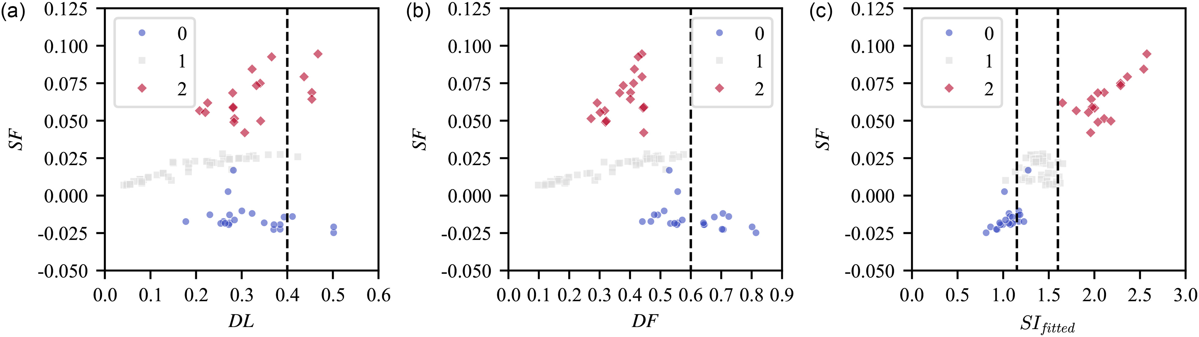
The relationship between these three types of flow fields and these empirical parameters that serve to classify is illustrated in Figure 4. The distribution of these empirical dimensionless parameters suggests that the dataset covers a wide flow range with no obvious bias. The key factor for judging a parameter’s classification effectiveness is whether it can show clearly separate values across different flow types, as illustrated by SF which successfully categorizes flows into three classes through its two critical thresholds (SF=0.005 and 0.040, marked by dashed lines in Figure 4a and b. In contrast, DL and DF demonstrate overlapping value ranges across three flow patterns, rendering them ineffective classifiers in this study. When both axes represent classifiable parameters, the data spontaneously clusters into three distinct groups. Due to the continuous nature of these dimensionless parameters, a proportional relationship emerges between them — a phenomenon evident in Figure 4c and d, where SI and AVDR demonstrate linear relationships with SF, confirming their utility as flow classifiers. These observations can be physically interpreted through the inherent mechanisms of SI and AVDR. SI characterizes spanwise loss variations to differentiate flow separations. Meanwhile, AVDR primarily reflects passage blockage effects. Specifically, 3D open corner separation induces endwall blockage, which amplifies midspan flow compression. Conversely, 2D separation (particularly choking condition) degrades axial flow performance at midspan. However, as evidenced by overlapping parameter values between Tag 1 (no obvious separation) and Tag 2 (3D open corner separation) flow fields in the dataset, both SI and AVDR demonstrate inferior discriminative capability compared to SF — where certain data points corresponding to 3D open corner separations share identical SI / AVDR values with no obvious separation cases.

Figure 4.

Relationship between flow separation and dimensionless parameters: SF, DF, DL, SI, and AVDR.

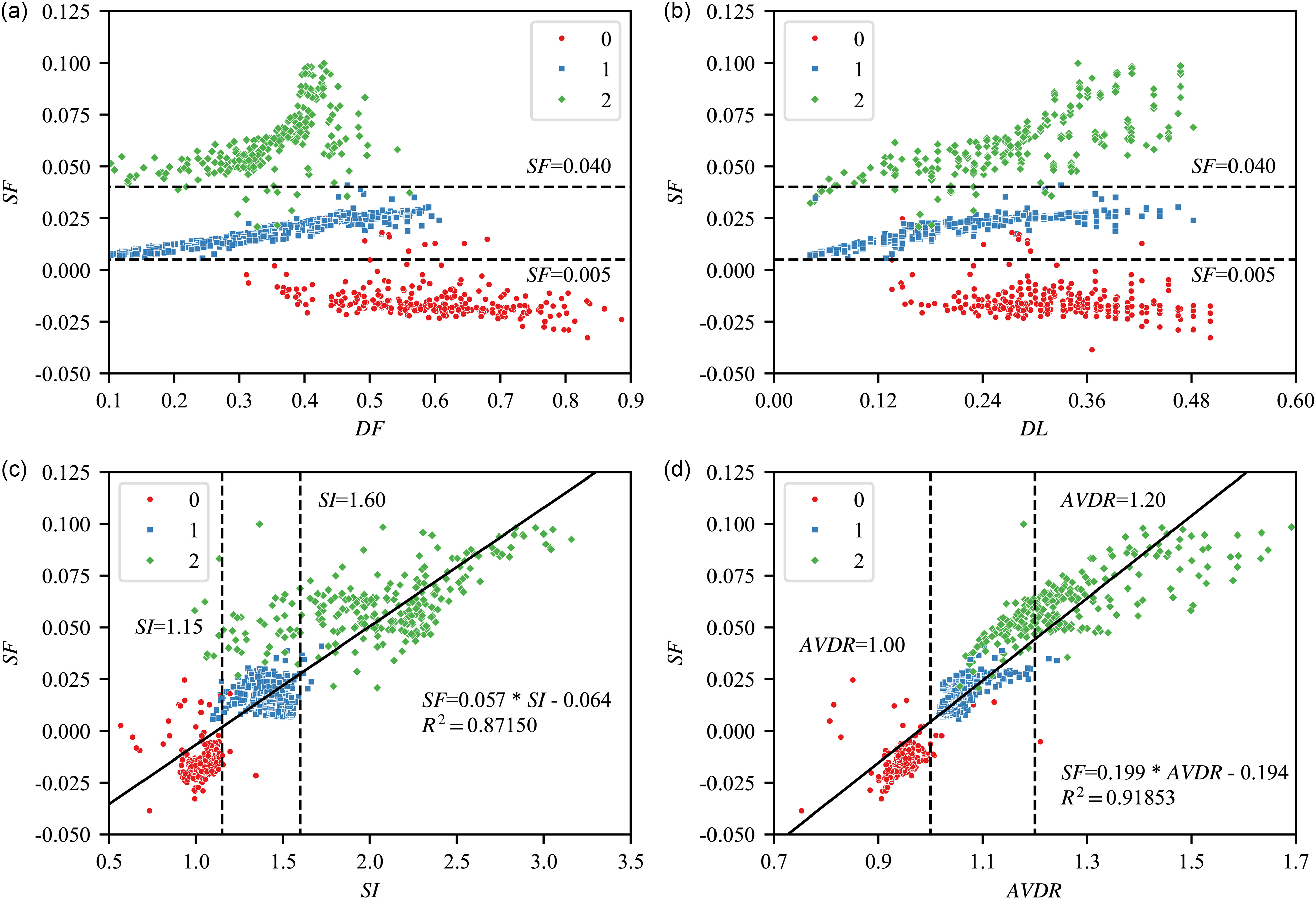
Table 2 directly presents the critical values of dimensionless parameters for flow separation classification. The classifying capability of the SF parameter is demonstrated in Figure 4a and b, which establish 0.005 and 0.040 as critical thresholds for distinguishing the onset of severe flow separation. The linear correlations observed in Figure 4c and d enable the derivation of SF’s critical thresholds from either AVDR or SI values. The SF thresholds calculated from AVDR correlations (0.005 and 0.045) demonstrate close agreement with the direct SF classification boundaries (0.005 and 0.040). The SF thresholds obtained through SI correlations (0.002 and 0.027) exhibit slight yet acceptable deviations.

In summary, while SF demonstrates the strongest flow classification capability in this dataset, its requirement for integration limits its applicability during preliminary design stages. Conversely, the most commonly used design parameters, DF and DL, exhibit the poorest classification performance. SI and AVDR show comparable classification capability, but similar to SF, they cannot be directly obtained from Equations 4 and 5 during the design phase. It should be noted that SI in Figure 4 can be directly derived by polynomial fitting of the design parameters (Zhou et al., 2023), which means that SI can serve as an input feature for the classification model. The expression is as follows:

where xi denotes six design parameters: DF, inlet Mach number, incidence, aspect ratio, passage contraction ratio and maximum thickness. The coefficients Ai, Bi,j and C were calibrated through least-squares regression using the same dataset as in this study.

Model construction and validation

Data-driven modeling not only improves the precision of modeling complex problems but also captures mapping-related information during input feature and model selection. To investigate the impact of model types and input features on classification performance, three models were constructed for comparative analysis.

This study employed an SVC model, a powerful supervised learning algorithm that separates data points of different classes by finding the optimal hyperplane in a high-dimensional space (Vapnik et al., 1997). SVC addresses linear and nonlinear problems by utilizing distinct kernels: the linear kernel for linear problems and the RBF (Radial Basis Function) kernel for nonlinear problems. Given that the SI can be derived from polynomial fitting (Zhou et al., 2023), the relationship between flow field classification and input features is anticipated to be nonlinear. To further examine the relationship, two models are constructed: one employing the linear kernel and the other utilizing the RBF kernel.

As previous studies (Wu et al., 2019; Yue et al., 2022) have confirmed, incorporating fundamental physical laws before training models may lead to better results (Karniadakis et al., 2021). This study follows a similar approach, drawing on the input features from previous empirical correlations (Lei et al., 2008; Yu and Liu, 2010; Zhou et al., 2023) and surrogate models (Wu et al., 2019; Yue et al., 2022). While the absolute values of AVDR and SI may not suffice for flow field classification, their inherent physical significance supports their use as input features. To further explore the influence of SI, the polynomial-fitted SI is included as an additional input feature in one of the models.

The three models are defined as follows:

The classification capability was validated using a test set comprising 10% of the total dataset, which was excluded from model training. Figure 5 presents the performance evaluation of the classification parameters on this test set. Given that both the flow fields and these critical dimensionless parameters were obtained through numerical simulations, we consistently use the three manually labeled tags as ground truth for assessment. When DL >0.4, it failed to distinguish among the three flow field types. For DF >0.6, only two-dimensional separation was observed, demonstrating DF’s classification capability as a two-dimensional limit loading indicator. Meanwhile, SIfitted outperformed both DL and DF, successfully classified three flow field types, exhibiting particularly strong performance in identifying three-dimensional open corner separation.

Figure 5.

Classifying parameter performances on the test set.

The data-driven model validation results on the test set are presented in Figure 6. Figure 6 compares the performance of the three models against the true labels using AVDR and SF as coordinate axes. The results demonstrate that the RBF kernel achieves better alignment with the true tags compared to the linear kernel, suggesting a nonlinear relationship between the input features and the flow field structure.

Figure 6.

Classification performance comparison across three models with true tag.

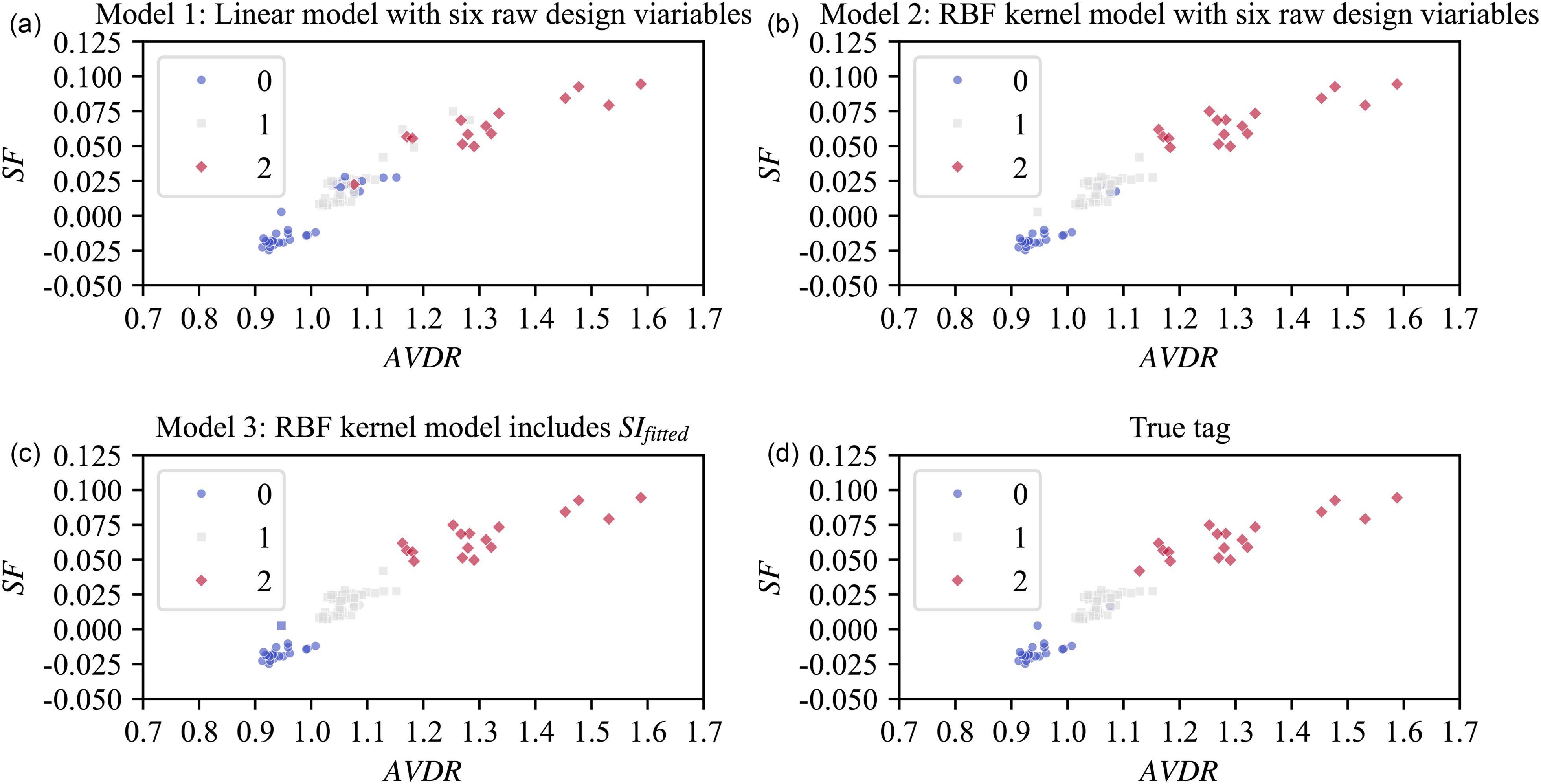
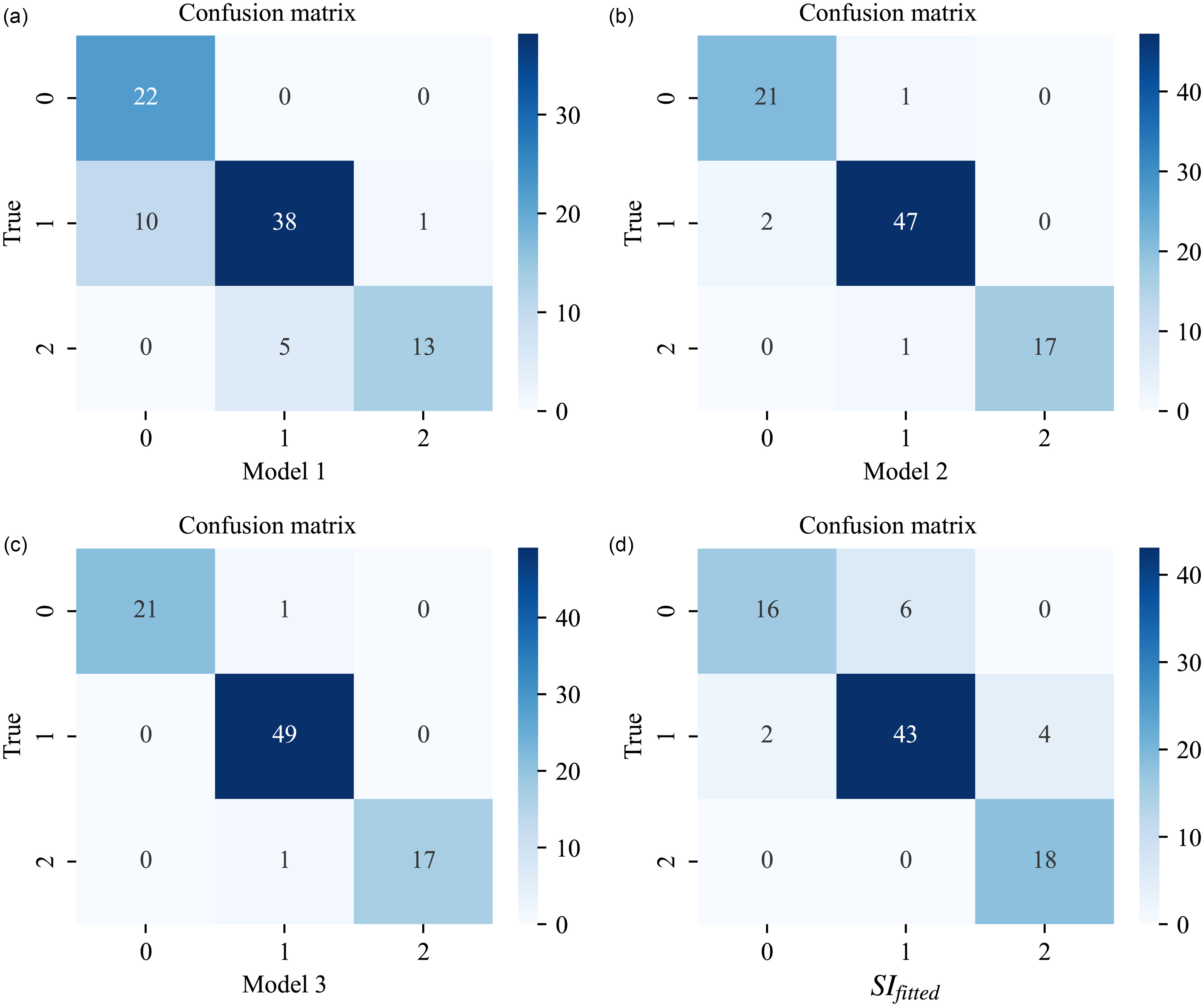
Figure 7 provides a confusion matrix for the three-class problem, where rows represent true classes and columns represent predicted classes. Each cell Cij shows the number of true class i samples predicted as class j, highlighting classification errors. Notably, confusion matrix (d) was generated by discretizing the SIfitted values into three classes based on the critical thresholds specified in Table 2, followed by comparison with the true tags. Analysis of the four classification results demonstrates that Model 3, incorporating the dimensionless parameter SIfitted, achieves best alignment with the test set’s true tags. This evidence confirms that the data-driven model outperforms classification using a single parameter, while simultaneously highlighting the value of dimensionless parameters with clear physical significance for enhancing model performance.

Figure 7.

Comparison of confusion matrices for three data-driven models and SIfitted.

Conclusion

This paper used a database of 889 linear stator cascades to train a data-driven flow field classification model. Numerical results were validated against experimental data to assess the reliability of the simulations. An analysis was conducted to investigate the relationships between five key parameters for evaluating flow fields. The fitted SI was incorporated as an input feature in the final model. Among three validated data-driven models, the nonlinear RBF kernel model incorporating the fitted SI yields the highest classification accuracy, while the linear kernel model utilizing only the six raw design variables performance worst. The following conclusions can be drawn:

Nomenclature

Subscripts