
Introduction
When a highly loaded compressor reaches its aerodynamic stability limit, disturbances arise and may develop into either rotating stall or surge – both prominent types of a stalling process in compressors.
Rotating stall (RS) manifests as a fluctuation of the mass flow over the circumference while the total mass flow rate is nearly constant. Areas of flow separation and thus reduced mass flow (stall cells) are clearly discernible and propagate with about half the rotor speed in the absolute frame of reference. The pressure rise collapses and the operating point may then remain in a semi steady state while stall cells rotate continuously which is referred to as steady rotating stall (SRS), showing a constant operating point with rotating stall cells. In case the stall cell and the operating point are unstable, it is called transient rotating stall (TRS).
Under certain conditions (for example a throttled plenum attached to the compressor) RS may initiate surge, resulting in a one dimensional mass flow oscillation over the full annulus. Hence, the total mass flow as well as the pressure rise coefficient pulsate. The time scales and amplitudes are larger than for RS. In a compressor map, a surge cycle is discernible as a counterclockwise rotating operating point. It is called mild or classic surge, if the mass flowrate remains positive and deep surge, when the flow direction is reversed for a part of the cycle.
In the past decades, significantly more research has been conducted on RS rather than on surge. Greitzer (1976) analyzed the characteristics of a surging compressor and developed a compression system model as well as the B parameter which takes into account the tip speed
Nearly two decades later Day (1994) underlined a lack of experimental data and limited information about flow conditions in axial compressors during surge and therefore carried out comprehensive measurements on a multistage low speed laboratory compressor. The results reveal that surge is always preceded by RS and its oscillation is independent of the system’s Helmholtz frequency. Hence, surge can be classified as a process of pumping-up and blowing-down the plenum chamber or a collapse-and-recovery process of the flow, more than a dynamic instability. Additionally, he proposed to include details of the compressor design into the B parameter. With pressure rise ΨPeak and flow coefficient ΦPeak at the peak of the characteristic this leads to
Day and Freeman (1994) compared the surge characteristics of a low speed compressor to those in a high speed machine with fixed geometry design (Rolls-Royce Viper Engine). They concluded that laboratory testing of low-speed compressors is an effective and inexpensive way of gaining insight into many aspects of the behavior of aero-engine compressors. However, when the Viper high speed machine surged at top speeds, the first cycles occurred with such violence that the flow reversal extinguished the combustion and the engine stopped. Thus, not much data during surge at top speeds was acquired.
Weigl et al. (1997) implemented an active air-blow-in-stabilization in a single stage transonic compressor to extend the operating range and described its impact on the performance. With active control, operating points beyond the stability limit were stabilized. When the control was turned off, the compressor fell into rotating stall or surge immediately. Weigel focused on the range extension by stabilization rather than detailed analysis of the surge mechanism itself.
Courtiade and Ottavy (2013) carried out an experimental study of surge precursors in a 3.5-stage high speed compressor and developed an active anti-surge control system to enhance near-surge measurements without falling into surge. However, as Courtiade pointed out, there is still a lack of experimental data concerning high speed and transonic compressors. This is due to high risks and costs, which high speed testing entails, especially for operation with highly loaded blades. Furthermore, investigation of unsteady aerodynamics requires extensive and costly instrumentation for data acquisition and safety monitoring.
As a result, detailed experimental data of in-stall operation or surge-cycles is still a valuable resource of information to improve the validity of numerical tools, especially for high speed compressors. Consequently, as Day (2016) concludes, there is a great need for high-speed testing. Particularly, studies dealing with surge occurring in a transonic compressor test rig are still rare, which highlights the originality of the surge phenomenon identified at the new Transonic Compressor Darmstadt. Its characteristics are to be elaborated in this paper.
Experimental setup
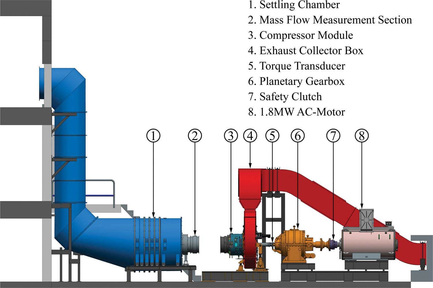
The analyzed data was acquired at the new 1.5-stage Transonic Compressor Darmstadt 2 test rig (TCD 2), shown in Figure 1. The compressor module represents a scaled front stage of a state-of-the-art industrial gas turbine compressor with variable inlet guide vanes (IGV) and a variable stator. The rotor, a bladed disc, is driven by a 1.8 MW electrical drive. This allows shaft speeds up to 20.000 rpm, resulting in a blade tip speed of approximately 400 m/s and pressure ratios up to 1.7. The rig provides a high modularity, enhancing short turnaround times between different rotors. It is equipped with extensive steady and unsteady measurement systems enabling investigation of compressor characteristics, unsteady aerodynamics and aeroelastic behavior of the compressor.
During the first measurement campaign comprehensive measurements were conducted, including steady-state and transient tests as well as multiple maneuvers beyond the stability limit. A detailed overview concerning test rig capabilities, performance and instrumentation as well as results of steady data analyses was elaborated by Kunkel et al. (2019).
As a part of this campaign 65 transient maneuvers causing stall were conducted for different speed lines and IGV settings. Therefore, starting from the last steady stable operating point of a speed line, the throttle at the diffusor exhaust was closed stepwise or continuously until the compressor reached its aerodynamic stability limit, manifesting different stall phenomena. To show their distinguishing characteristics, two exemplary measurements are analyzed in detail.
Instrumentation and methodology
In the following section an exemplary stall maneuver with a pronounced SRS is analyzed to introduce the methods and instrumentation. This maneuver was carried out at 92% of design speed (N 92) and nominal IGV setting.
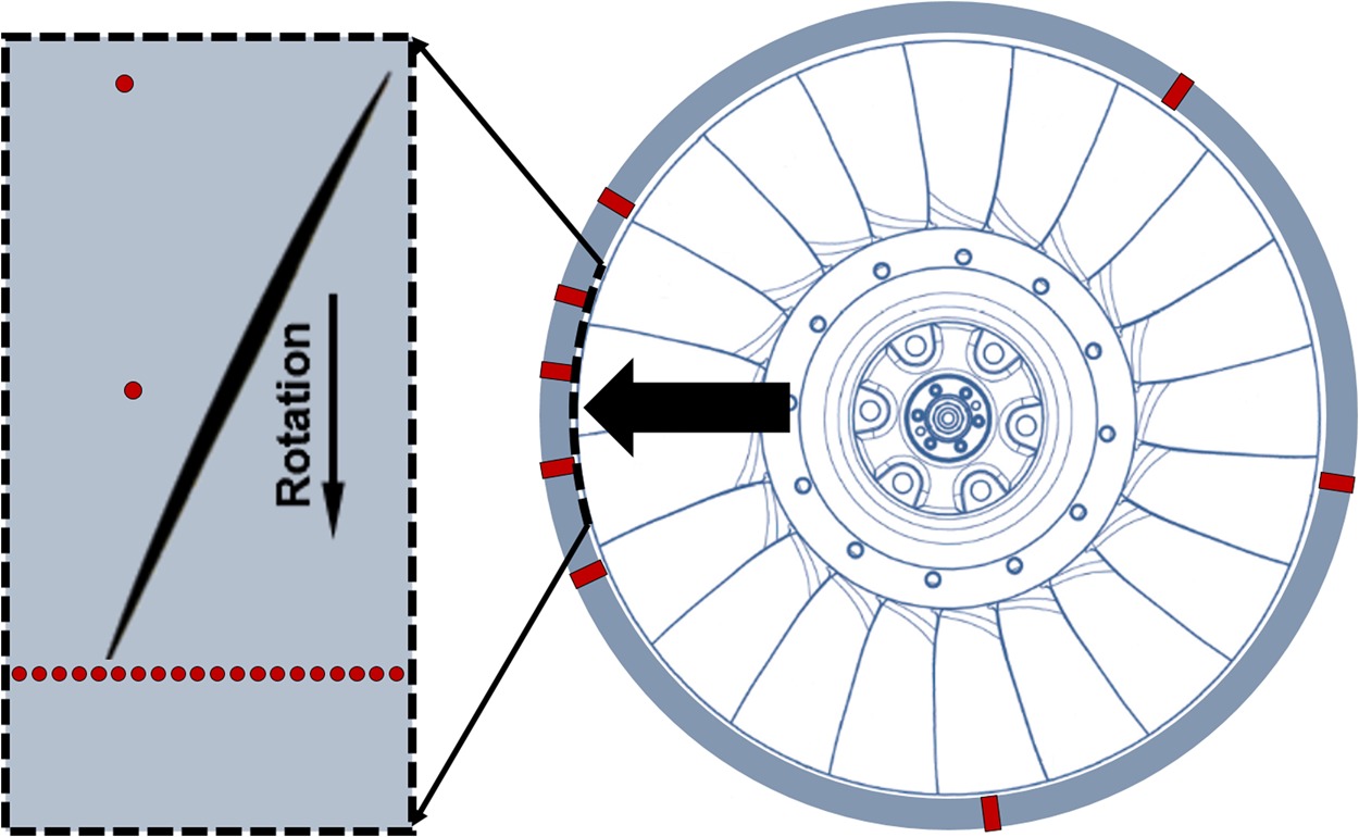
The unsteady measurement systems include, for example, strain gauges on blades and vanes as well as piezo-resistive static wall pressure transducers (WPT). The sampling frequency fsmpl of the WPTs is 500 kHz, with a low-pass filter at 70 kHz. WPTs are circumferentially distributed at the rotor leading edge and arranged as an axial array over the rotor, as sketched in Figure 2. Subsequently, the applied methods are presented for the example of rotating stall with a change of cell count.
As suggested by Cumpsty (2004), the total-to-static pressure rise coefficient Ψ was determined as the difference of the revolution-wise averaged pressure
Furthermore, it is normalized with the highest Ψ determined in this measurement, Ψref. In this investigation, both events, stall onset and emergency bleed valve opening, can be reliably identified by a sudden drop of Ψ, as shown in Figure 3.
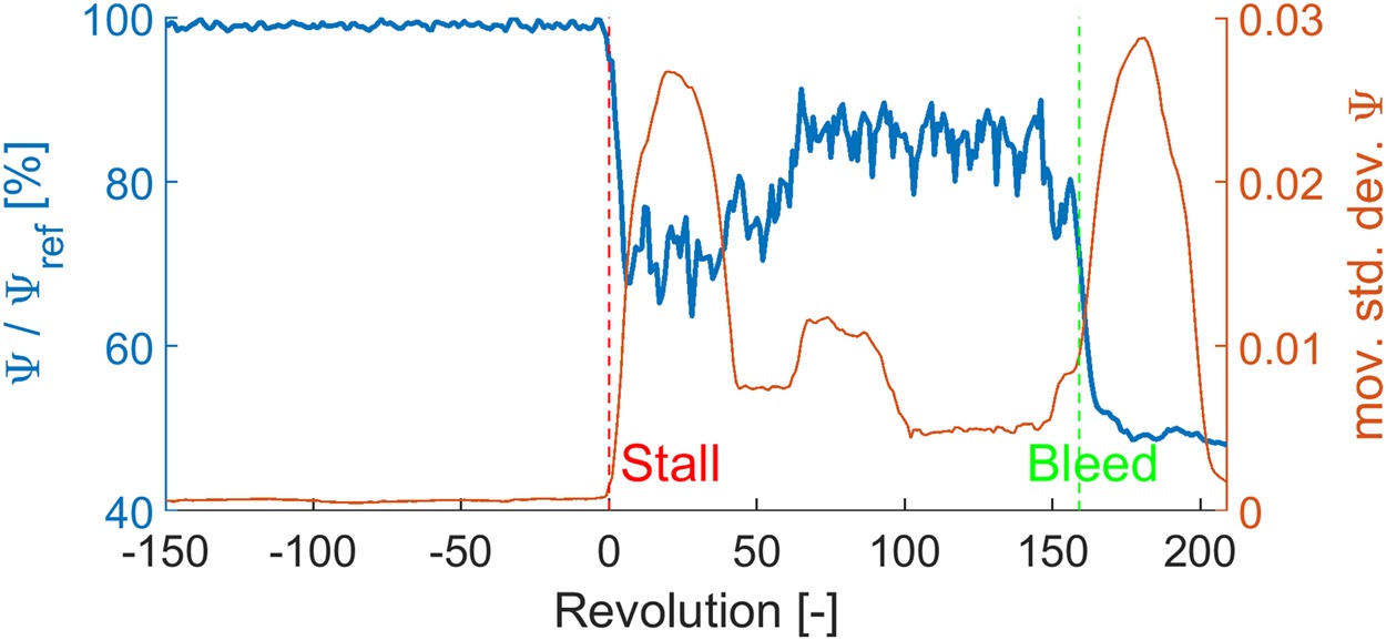
Based on that, a stall onset is detected by an algorithm, if the moving standard deviation of Ψ surpasses a threshold value with a positive slope. With this method, the stall onset and bleed opening of all transient stall maneuvers are identified with an accuracy of less than 2 revolutions and used as reference mark. Setting the stall onset as revolution 0 enhances an automated and well comparable analysis of numerous stall maneuvers.
To isolate non periodic fluctuations, the ensemble average of the last 30 revolutions before stall onset is subtracted from the WPT-signal. A similar method is for example described by Brandstetter et al. (2019). The deviation Δp is calculated by subtracting the ensemble average of the last 30 revolutions (counter m) before stall onset revolution (Nstall) from each sample i of a revolution n.
The resulting spectrum of a signal at the rotor leading edge, plotted in Figure 4, allows to identify pressure oscillations with related frequencies and amplitudes. The sudden stall onset is always indicated by strong broadband fluctuations and mostly by several prominent peaks at distinct frequencies. In this case, 4 peaks appear in revolutions 0–50 and are discernible in the peak-hold diagram, which shows the maximum frequency amplitudes over the analyzed period. Normalized with the rotational frequency of the rotor, the highest peak can be expressed as engine order (EO) 1.22. After revolution 50, the highest peak shifts to EO 0.57 and related harmonics appear (EO 1.11 and EO 1.73).

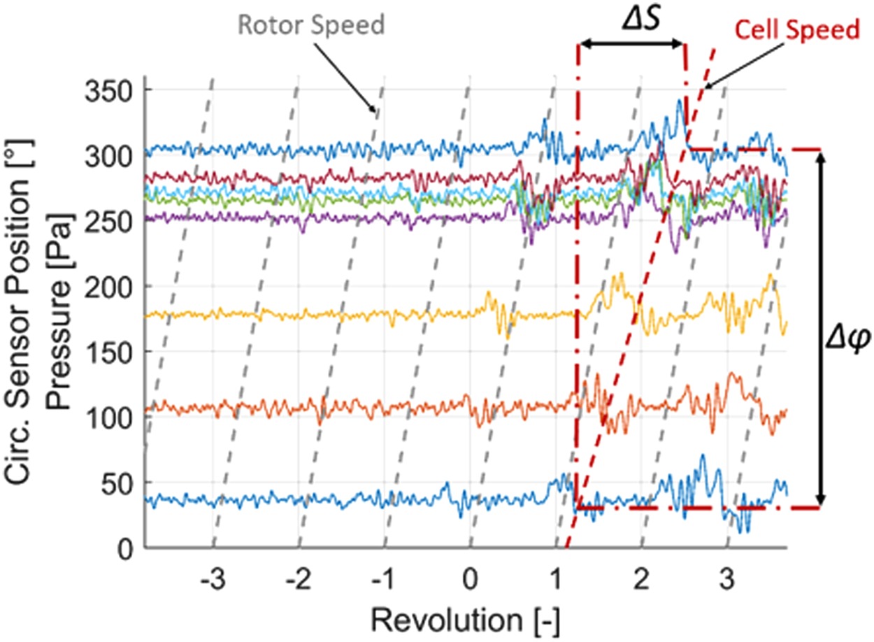
In order to derive the circumferential propagation speed of disturbances, WPTs are distributed around the circumference of the outer casing close to the leading edge, as illustrated in Figure 2. A rotating stall cell has a characteristic pressure fluctuation or “foot print” when passing by the sensors. Figure 5 shows the development of the first stall cell near revolution 0. The fluctuation in the signals is shifted by a count of samples ΔS or time lag Δt due to the angle Δφ between two sensors. The rotational frequency of a propagating cell fprop is equal to the ratio of swept angle Δφ and time Δt.
To determine the time lag
The cross-correlation is performed over signal sections (e.g. 2 revolutions) and for all sensor combinations. If a disturbance propagates, the correlation of one combination shows peaks for different shifts. In order to avoid this aliasing, the minimum of the cross-correlation of all sensor combinations is determined, as described by Brandstetter et al. (2018). For a given propagating disturbance, all sensor combinations show a high correlation for fprop. Thus, the combined correlation minimum shows a peak indicating the propagation speed for the analyzed window of revolutions.
To obtain time resolved information about the correlation, this analysis is performed for every signal section and then gathered in a propagation-speed spectrogram. It shows the minimum correlation of all sensor combinations for a bandwidth of propagation frequencies, plotted over revolutions in Figure 6.
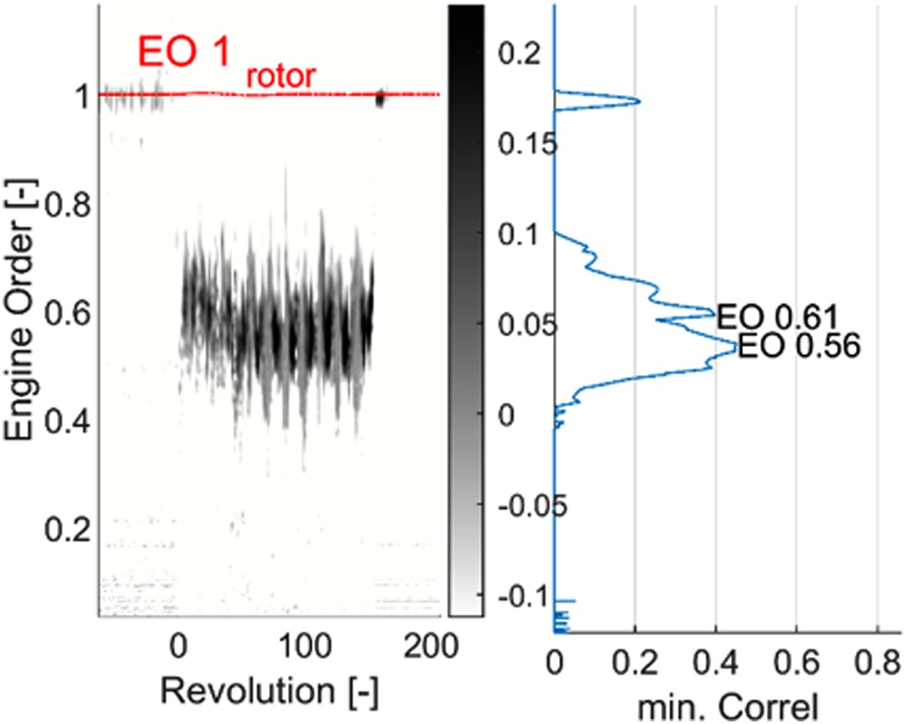
When the correlation minimum is high (dark spots), a propagation speed is indicated. In this case, the average speed for revolutions 0–50 shows a high peak for EO 0.61, which is half of the related EO 1.22 in Figure 4. This indicates two rotating cells. Additionally, since more peaks and strong disturbances are visible in Figure 4, it leads to the assumption that several smaller and unstable stalled areas propagate and superimpose with the two main cells. After revolution 50, the average speed decreases slightly, approaching the highest peak for EO 0.56, matching with EO 0.57 in Figure 4. This marks the presence of one stable rotating stall cell and indicates a fusion of all disturbances to one large cell at approximately revolution 50.
To visualize aerodynamic phenomena at the rotor tip, WPTs are also mounted in an axial array in the casing at one single circumferential position (see Figure 2). Their signals are sorted revolution wise and mapped into a rotor-relative wall pressure field. The deviation Δp of the current pressure field is calculated as introduced in equation 5 and is furthermore normalized with pdyn. This method enhances a clearer distinction of stalled areas, disturbances and shock fluctuations.
Figure 7 shows the revolution wise sorted pressure deviation of the axial array for two different aerodynamic conditions. Revolutions −1–8 show a clearly distinguishable start of RS, with stalled sections emerging (as already evident in Figure 5), growing rapidly and splitting into several cells. This agrees with the findings of Figure 4 showing several frequency peaks, caused by multiple cells and stronger broadband fluctuations than after revolution 50. The higher propagation speed in Figure 6 is also consistent, since multiple smaller cells tend to rotate faster than larger cells.
Revolutions 130–140 show a single and stable rotating stall cell appearing slightly more than once per every two revolutions. Counting the cell passings from revolution 131–138 results in EO 0.57. This agrees with both peaks in the spectrogram and the identified propagation-speed. The supposed fusion of several small cells into one also correlates with an average rise of Ψ at approximately revolution 50 in Figure 3.
Experimental results and discussion
Since the new TCD 2 test rig was designed based on the well-known TCD, a similar behavior concerning stall characteristics was expected. The TCD has been operated by the Institute of Gas Turbines and Aerospace Propulsion since 1994 and its rotors, mostly representative for aero engines, are throughout prone to aero-elastic effects such as flutter, non-synchronous vibrations and related aero-mechanical coupling. This is reported in numerous studies, both experimentally and numerically (Holzinger et al. 2016; Brandstetter et al. 2018; Jüngst 2019; Möller 2019).
However, the characteristics near and beyond the stability limit of the TCD 2 were surprisingly different and noticeable in two aspects.
The rotor neither shows any non-synchronous vibrations (NSV) with aeromechanical coupling nor typical striking aerodynamic precursors prior to stall. In most cases, it approaches the aerodynamic stability limit but not the structural, given by high blade vibration amplitudes.
The TCD 2 indicates a variety of acoustic and convective phenomena in the stalled operating point. One of them emerges as a periodic occurrence of rotating stall, hence transient rotating stall (TRS), causing strong fluctuations of the total-to-static pressure rise coefficient and alterations of the mass flow with a low frequency, typical for a surge. This was never observed at the TCD and will be described below.
The surge phenomenon
In this section, a stall maneuver with a pronounced periodicity during TRS is analyzed, revealing several characteristics of a surge. Based on the conclusion drawn by the authors, in the following this phenomenon is referred to as surge. This measurement was acquired at design speed (N 100) and nominal IGV setting.
The most prominent characteristic can be found in the periodic course of the total-to-static pressure coefficient Ψ when reaching the aerodynamic stability limit. As shown in Figure 8, Ψ drops and instantly develops a periodic fluctuation of approximately 40% of the total pressure rise. The upper peak of most cycles is higher than the mean value before surge onset. The engine order can be determined with equation 7.
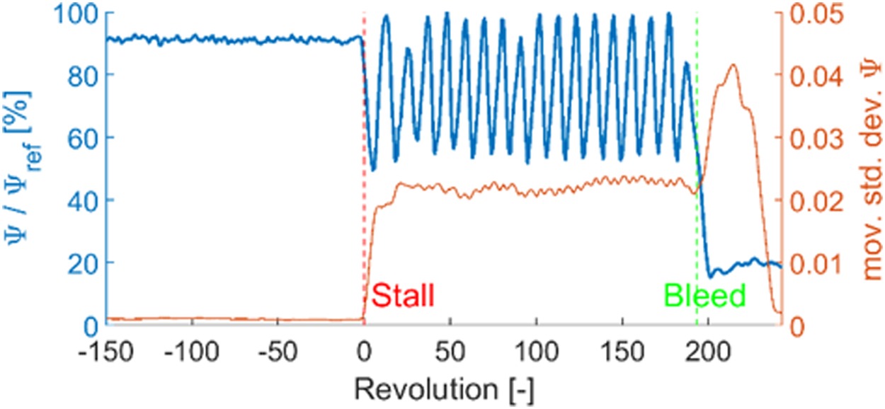
This agrees well with the largest peak in the spectrogram from a WPT at the rotor leading edge (see Figure 9) at EO 0.1, arising instantly after the stall onset. For all measurements, this periodicity lies from EO 0.06–0.1. Before stall onset, no significant amplitude peaks could be detected which would typically indicate aerodynamic precursors like modal or acoustic waves. However, during stall there are two short-lived peaks at EO 0.71, indicating a rather fast rotating disturbance or stall cell (revolution 20 and 90).

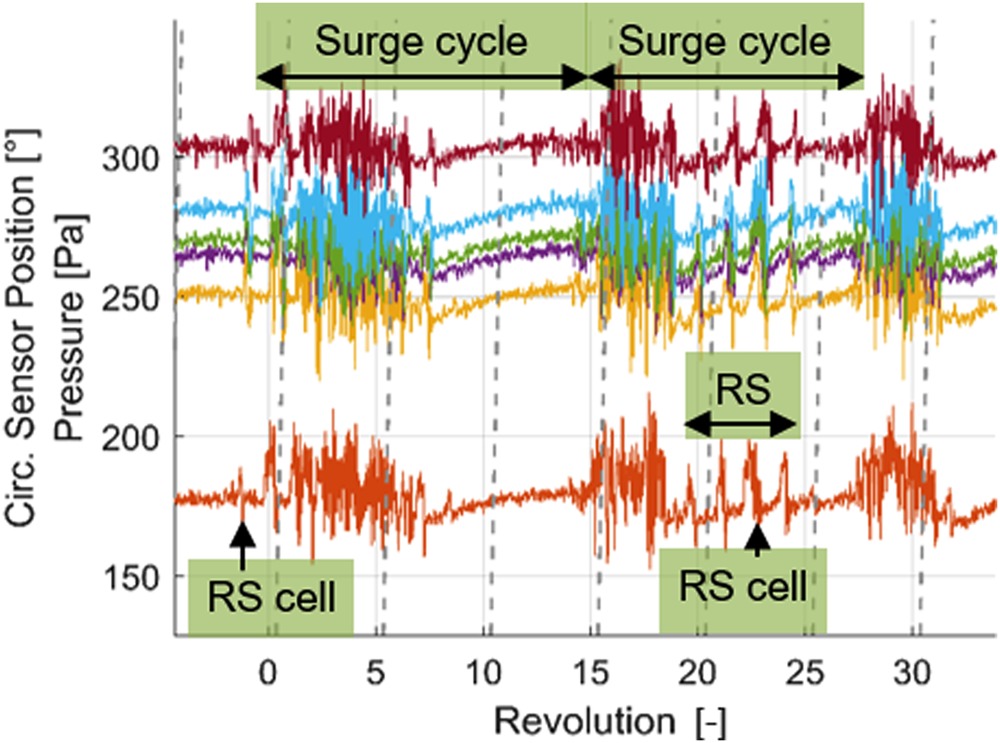
Data from the circumferential distributed WPTs confirms this interpretation. Figure 10 shows a fast growing, propagating stall cell (revolution −1) leading to a first surge cycle with a subsequent recovery lapse free of disturbances. In the second cycle, a stall cell arises during recovery (revolutions 18–25). This repeats at revolution 90 – the related peak again appears in the spectrogram in Figure 9.
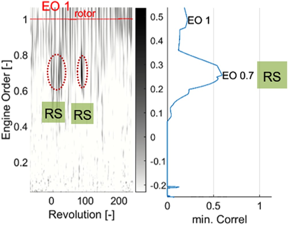
These rotating cells are discernible in the propagation-speed spectrogram in Figure 11. At revolution 20 and 90 it shows higher correlation at about EO 0.7 which, combined with Figure 9, indicates a rotating stall cell. Furthermore, each surge cycle leads to high correlation values for the upper frequencies (grey vertical stripes), which is due to the larger planar pressure fluctuations that are in phase over the circumference, thus resulting in a high correlation for
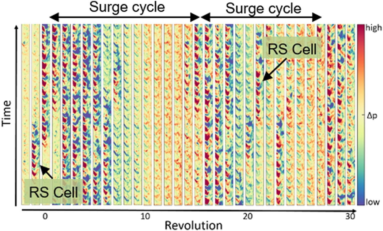
The wall pressure deviation fields of the axial WPT array in Figure 12 show the stall onset with a rotating stall cell and the first two surge cycles – the first one with an undisturbed recovery and the second one with a stall cell remaining after the cycle lasting 4 revolutions. The surge frequency can be determined by counting the cycles in a longer signal frame, resulting in EOsurge = 0.091.
These findings confirm the abrupt nature of surge onset in highly loaded transonic compressors, as mentioned by Day (2016) referring to the high-speed Viper compressor. They also are in line with Tryfonidis et al. (1995), who found that in all their compressors rotating stall always precedes surge. Moreover, these results show that both phenomena might alternate. This is observed in numerous maneuvers of the current study.
As the pressure fluctuation amplitude approaches 40% of the pressure rise (see Figure 8), significant alterations of the operating point in terms of pressure rise and possibly mass flow were expected by the authors. The latter is a necessary characteristic to classify this phenomenon as surge.
Unfortunately, the systems for the acquisition of total pressure rise and mass flow are not intended for unsteady measurements so that the typical surge hysteresis could not be recorded. Nevertheless, the determined mass flow
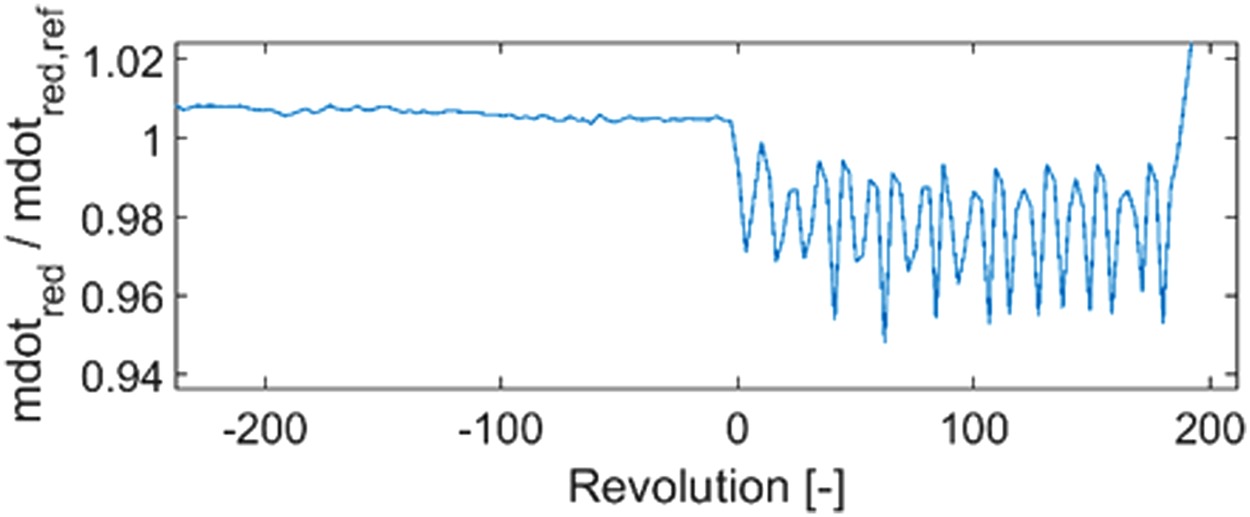
However, the amplitude of the underlying measured pressure oscillations is reduced by the volume and damping of the connection tubes in the steady measuring chain. Therefore, the mass flow oscillations are presumed to be significantly larger in reality than the output of the steady data. This is to be verified in the following section.
Determination of the OP hysteresis amplitude
To enhance unsteady acquisition of the mass flow fluctuation due to a potential surge cycle, a piezo-resistive pressure transducer placed in a Kiel Head probe (KH) and a WPT are mounted in the compressor inlet duct. This allows to measure the local total and static pressures (
As
Then, an additional stall maneuver was conducted for the same configuration as the one described above leading to similar observations. Combining the determined mass flow with Ψ, a left-rotating surge hysteresis is clearly recognizable in Figure 14. From the last stable operating point (OP), where steady (OPstat) and unsteady values (OPKH,WPT) match, the compressor falls into surge for 4 cycles until the back pressure is released by opening the bleed valve. The compressor then stabilizes at a lower point of the speed line and the OPs match again.
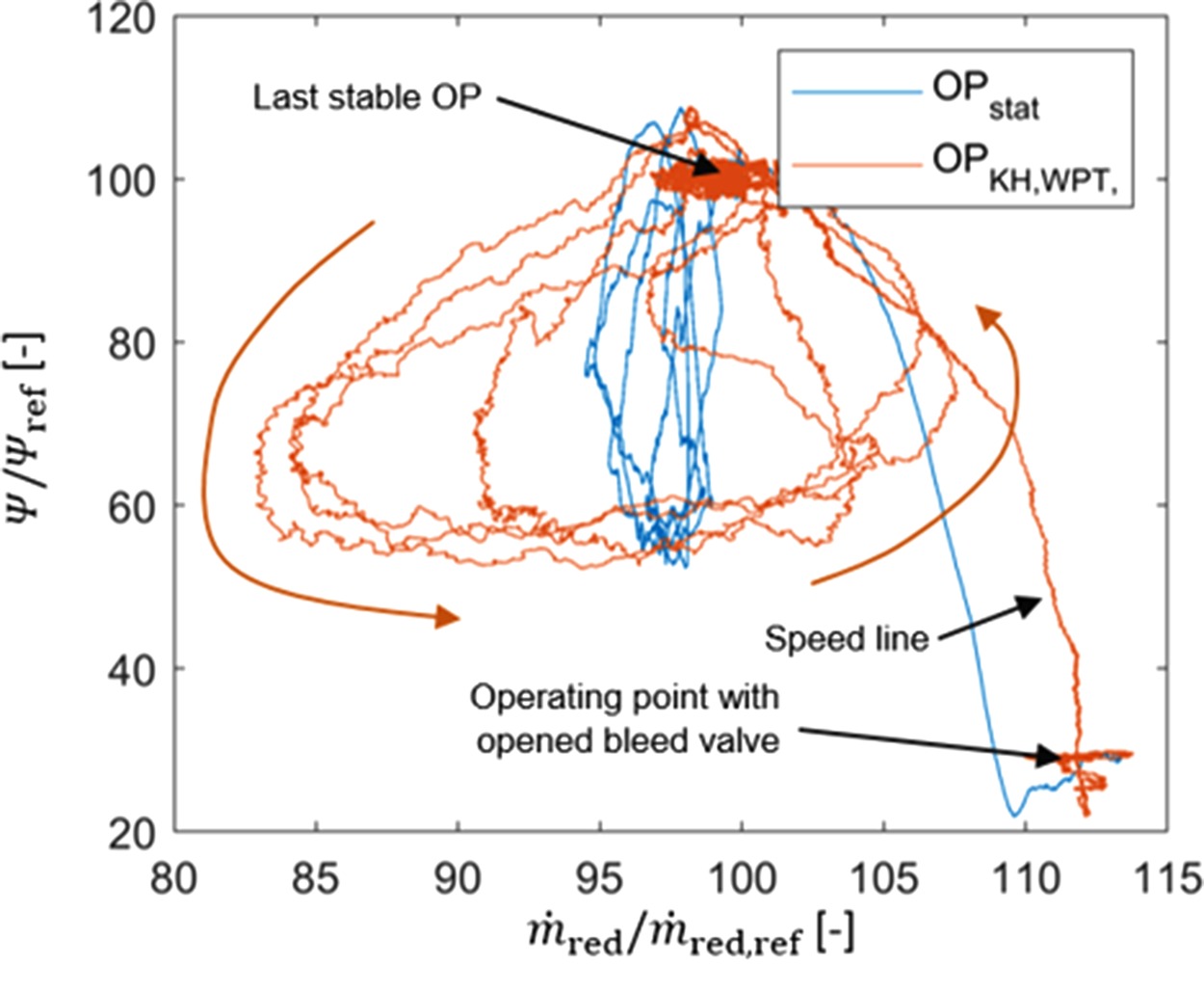
The fluctuation amplitude of OPstat is comparable to Figure 13 and indicates 5% for the mass flow and about 42% for the pressure rise, as it was expected for an identical phenomenon. The hysteresis of the unsteady measurement (OPKH,WPT) shows a fluctuation of approximately
Furthermore, it suggests that similar amplitudes were existent in the maneuver where the unsteady measurement of the mass flow was not yet realized. As a consequence, the authors come to the conclusion that the observed phenomenon described in the detailed analysis above is a surge with a hysteresis as described by Greitzer (1976) or Day (1994).
Rig Geometry Influence and B Parameter
Since the design and the operating parameters of TCD 2 are very similar to those of the TCD, a rig where surge was never observed, it was not expected to develop this phenomenon. Furthermore, the plenum downstream the compressor (duct and diffusor) is small. According to Cumpsty (2014), “with no plenum there is no mass storage and the compressor cannot surge in the sense of causing oscillations of mass flow, but the flow ‘collapses’ and readjusts into a rotating stall.”
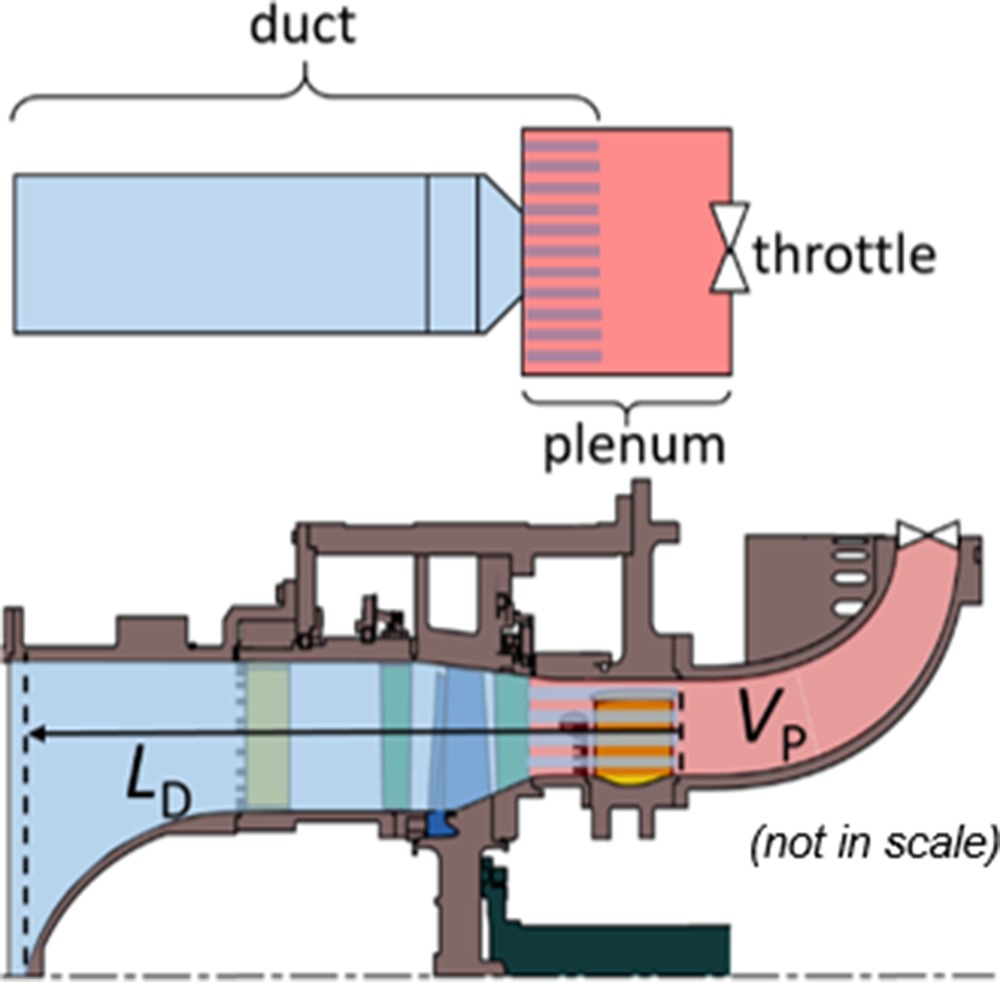
Although the parameters for a determination of the B parameter are only approximately quantifiable, the compression system was reduced to a duct with length LD (from the nose cone to diffusor inlet) and a plenum VP (the volume between outlet stator and throttle) as shown in Figure 15. This parametrization leads to a B = 0.65 at design speed which indicates a value of Bcrit, lying below 0.65. The actual compressor specific Bcrit is objective of future investigations.
Regarding the understanding of B and B′, the high tip speed and pressure ratio of the TCD 2 increase the probability of surge. Thus, the volume of the short duct downstream the compressor combined with the diffusor appears to be sufficiently large to provoke compressibility effects of a “plenum” and thus can lead to surge, as the phenomenological observations indicate.
However, the question remains why there is such a difference between two similar test rigs concerning the aerodynamic characteristics beyond the stability limit. A detailed comparison of geometry, B and operating parameters could be object of further research.
Relative occurrence of transient rotating stall
The 65 stall maneuvers mentioned above were assessed concerning the type of stall phenomena. Due to the subsequent implementation of unsteady mass flow measurement, the unsteady operating point trajectory (as shown in Figure 14) is not available for these measurements, hence it is not possible to identify or prove surge for this data set.
However, based on the course of the pressure rise coefficient and the analysis of pressure spectrograms and propagation speeds, several types of stall were characterized. Yet, this paper focuses on the occurrence of RS which was subdivided into steady rotating stall (SRS – Ψ is nearly steady with rotating stall) and transient rotating stall (TRS – Ψ fluctuates with low frequency, approx. EO = 0.1, and an amplitude of at least 15% of pressure rise during stall). The Ψ course of the latter is similar to the one of surge, hence surge occurrence is included in the TRS count. Other phenomena (e.g. acoustic resonances) are mentioned in this figure, but will be object of future publications. Furthermore, in most measurements the phenomena are not observed exclusively, but occur in succession. The relative occurrence is shown in Figure 16 for different speeds and IGV settings.
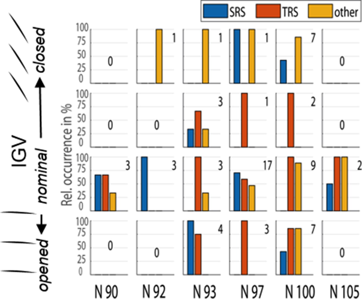
It becomes clear, that this test rig configuration develops TRS for a wide operating range which in some cases actually was a surge as e.g. the case described above. The actual operating range with surge occurrence should be assessed in future measurement campaigns.
Since the rotational speed influences the B parameter and thus the tendency to surge, a relation to the Ψ fluctuation amplitude of TRS is assumed. Therefore, those measurements are selected, that show TRS or surge but no (or only weak) SRS or acoustic or convective mechanisms. Their Ψ signal is cut to the section between stall and bleed and low-pass filtered above EO 0.1. This allows to determine the flank heights (fh), as indicated by the dashed lines in the upper diagram in Figure 17. These values are plotted as single points over the corresponding rotational speed in the bottom diagram. Additionally, the average values (circles) of maximum and mean flank heights are calculated for every speed and a best fit line is determined.
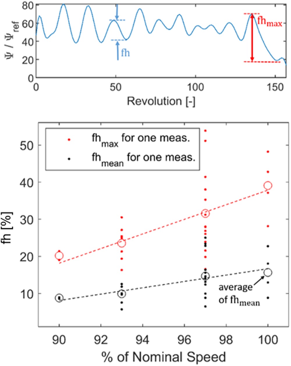
The mean and maximum amplitude of low frequent pressure fluctuations during TRS tend to increase with rising rotational speed which matches well with the expectations, the definition of the B parameter and hence Greitzer’s (1976) detailed studies on a low-speed compressor. This also may indicate that TRS shades into mild surge and or even surge when the B parameter is increased.
Conclusion and outlook
Extensive unsteady data was acquired during the first measurement campaign at the new Darmstadt Transonic Compressor test rig (TCD 2). This study shows some of its characteristics beyond the stability limit and detailed aerodynamic analysis of surge.
The characteristics near and beyond the stability limit of the TCD 2 differ from those of a very similar test rig at the same institute. The rotor does not show any typical NSV with aeromechanical coupling nor typical striking aerodynamic precursors prior to stall. In most cases, it approaches the aerodynamic stability limit, but not the structural given by high blade vibration. This is most likely due to the friction between blade and disc.
However, the compressor shows a variety of acoustic and convective phenomena beyond the stability limit, providing a valuable data set for numerical validation of in-stall operation and related physical mechanisms.
Besides SRS for a wide operating range TRS was observed. In some cases the amplitudes of the pressure fluctuation were particularly high and showed a periodicity.
Through further analysis typical characteristics for surge could be observed. Fluctuations of the pressure rise and the mass flow were identified. These cycles without reversed flow lead to a counter-clockwise rotating hysteresis of the operating point.
The compressor geometry and the operating parameters are very similar to a transonic rig at the institute where surge has never been observed.
With rising rotational speed, the average flank height of the low frequency pressure oscillations of TRS increases which indicates a shading of TRS into surge with rising B.
Further arising phenomena have been characterized and underlying aerodynamic and acoustic mechanisms were identified. These will be subject of future publications. A global and detailed survey of the stall phenomena in this test rig could enhance the understanding of stalled aerodynamics in a transonic compressor and provide detailed data for validation and improvement of numerical tools. This would allow a more precise prediction of aerodynamic stall behavior as well as related blade loading and potentially associated vibrations.
Nomenclature
EO
Engine order
IGV
Inlet guide vane
fh
Flank height
KH
Kiel head probe
N
Percent of nominal speed
OP
Operating point
RS
Rotating stall
SRS
Steady rotating stall
TCD 2
Transonic Compressor Darmstadt 2
TRS
Transient rotating stall
WPT
Wall pressure transducer
A
Cross-section
B
Greitzer’s B parameter
i
Sample
f
Frequency
K
Compressibility
L
Length
p
Pressure
Mass flow
n
Revolution
Nstall
Stall inception revolution
S
Samples
t
Time
utip
Blade tip speed
V
Volume
[…]P
Plenum
[…]D
Compressor Duct
[…]s
static
[…]smpl
samplerate
[…]stat
steady
[…]t
total
[…]prop
Propagation
[…]rotor
Rotor
[…]KH,WPT
Kiel Head, Wall Pressure Transducer
[…]red
reduced
[…]ref
reference
φ
Angle
Φ
Flow coefficient
Ψ
Total-to-static pressure rise coefficient
Standard deviation