
Introduction
During the development of Low Pressure Turbines (LPT) in modern high bypass aircraft engines, there are severe requirements for improving aerodynamic efficiency and weight reduction, in order to reduce fuel burn of aircrafts. From a perspective of aerodynamic design, the former can be accomplished by sophisticated designs to minimize the total pressure loss, while the weight can be reduced by high-lift design with reduced number of blades (Hodson and Howell, 2005). Although these two design directions are important, it is difficult to realize them at the same time, especially for modern LPT blades.
Because the LPT blades often have small chord length and generally work under low density, their Reynolds number becomes low enough to have laminar boundary layer and transition into turbulence (Mayle, 1991). The laminar boundary layer tends to separate far easier than turbulent one, especially in the high lift designs in which the flow on the blade suction surface is dominated by adverse pressure gradient. The occurrence of laminar separation and its state have strong dependency of Reynolds number and various flow disturbances such as free-stream turbulence intensity, incoming wakes from upstream blades, and potential interaction with downstream blades. In addition, when the laminar separation does not reattach on the blade surface, the loss significantly increases from attached conditions. Such undesirable burst separation bubble has to be avoided in design.
Since LPT blades incorporate highly sensitive laminar and transitional flow phenomena, an accurate prediction of the aerodynamic performance under transitional regime is essential for successful design. Recently, first-principal eddy-resolving simulations such as Direct Numerical Simulation (DNS) and Large Eddy Simulation (LES) have been advantageous methods over Reynolds-Averaged Simulation (RANS) for capturing laminar-turbulent transition and wake mixing. Despite its high computational cost, DNS and LES are useful not only for quantitative assessment of losses and their origins, but also for obtaining insights for further improvement of RANS turbulence model or low-order integrated model in preliminary design such as loss model. Various CFD codes have been developed and tested on turbomachinery cascades (Medic and Sharma, 2012; Sandberg et al., 2015; Bhaskaran et al., 2017; Bolinches-Gisbert et al., 2020). Recently, data-driven improved RANS models were actually developed based on statistics or flow fields by DNS or LES (Zhao et al., 2020).
Toward future use in aerodynamic design, this paper presents detailed validation of Large Eddy Simulation (LES) methodology. The validation is conducted over three LPT blades which have different blade loading distributions. In the first half of the paper, test blade properties, reference experimental data, and numerical methods are sequentially introduced. Then the transitional phenomena are described in detail for each cascade through comparison with the experimental data. Based on the discrepancy found in the comparison, additional sensitivity studies are conducted on the inflow turbulence and computational setups in order to further improve the LES prediction.
Test cascades
The test cases adopted in this paper are based on low speed cascade tunnel tests conducted in Iwate University (Funazaki et al., 2019; Okamura et al., 2019). The tests were conducted with 7 blades, whose axial chord and span lengths were 100 and 254 mm, respectively. Although incoming wakes can be modelled by a wake generator, the present study focuses on the cases without wakes in order to make the problem as simple as possible, which is the first step before including multi-stage effects. The Reynolds number, defined by the true chord length and exit flow velocity, was 1.0 × 10⁵. The inflow turbulence intensity was reported as around 1.2%. For more detailed information, please see the references.
Figure 1 shows three test cascades and their loading parameters. Design A is low-lift and fully laminar design, while design B and C are moderate- and high-lift design with boundary layer transition. Specifically, design C has an apparent laminar separation bubble and its transition on its suction surface. These cascades have different pitch width, but the inflow and outflow angles are almost the same among them.
Figure 1.
Test cascades and aerodynamic measurement stations. Note that the figures are intentionally deformed due to confidential reason.

The cascades are characterized by Zweifel loading factor (Zw). The Zw expressed by Equation 1 is interpreted as a non-dimensional tangential force acting on the blade. It is commonly accepted that the blade of Zw > 1 can be regarded as a high-load design.
Evaluation of aerodynamic characteristics
Figure 1 also shows aerodynamic measurement stations around the cascade. Two local one-dimensional coordinates x and
All pressure-related coefficients are nondimensionalized by the dynamic pressure on STN2. The total pressure loss distribution defined on STN2 is evaluated by the local loss coefficient
The cascade loss coefficient
Finally, the static pressure coefficient
Numerical method
High-order overset CFD code
The CFD code used in this study is PT3D, which has been developed in the University of Tokyo. It has been designed and used for unsteady flow simulations in turbomachinery aerodynamics and aeroelasticity research. The LES methodology in PT3D is based on compressible Navier-Stokes equation discretized by 4th order optimized compact finite difference method. Time marching is conducted by a 2nd order implicit scheme with Newton iteration and block ADI relaxation. In order to avoid numerical instability, 8th order tridiagonal low-pass filter (Visbal and Gaitonde, 2002) combined with time-consistent rescaling (Edoh et al., 2018) is applied at the end of every timestep with a filter coefficient of 0.495. An overset mesh technique is applied to realize high flexibility for complex geometry and parallelization. In order to improve interpolation accuracy between meshes, a new interpolation using radial basis function was developed, whose error was comparable to those in high-order Lagrange interpolation (Tateishi et al., 2018). The code has been validated and tested on various turbulent flows (Tateishi et al., 2017): homogeneous isotropic turbulence, channel flow, T106 LPT, NASA Stator 64B compressor, and transonic fan cascades.
The present simulation belongs to a class of implicit LES, and sub-grid scale physics such as kinetic energy dissipation are not explicitly modelled. This is because the tridiagonal filtering operation provides sufficient amount of dissipation for high wavenumber region, which was confirmed through a test case of decaying isotropic turbulence (Tateishi et al., 2017). Additional dissipation by any sub-grid scale models may deteriorate computational result especially for the velocity profiles of turbulent boundary layer.
Numerical setup and boundary conditions
Figure 2a shows typical CFD mesh used in this study. This configuration mimics two-dimensional flow away from endwalls, which is composed of a blade and background meshes. This periodic simplification is justified because the flow from 40% to 60% span height did not interact with the endwall flow and was almost uniform in similar experimental setup in the same tunnel. The inlet and outlet boundaries are located at 1 axial chord away from the blade. Both pitchwise and spanwise ends are connected periodically, where the spanwise width is chosen to
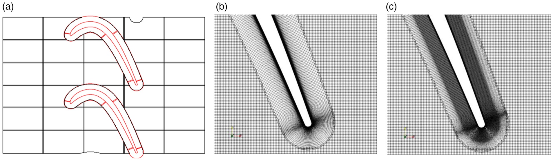
Local one-dimensional non-reflective boundary condition (Poinsot and Lele, 1992) is applied in order to supress unphysical reflection. The boundary values are solved using local one-dimensional inviscid (LODI) equations, where the incoming characteristic wave terms are controlled by the forcing terms using the specified variables (Yoo et al., 2005). The LODI equations of entropy, total temperature, and inflow angles are solved with the target values at the inlet, while the static pressure at the outlet is similarly handled (Tateishi et al., 2018). Inflow turbulence is modelled by divergence-free synthetic eddy method (Poletto et al., 2013), wherein the inflow turbulence intensity and length scales are specified to Tu = 1.0% and
Mesh and statistical convergence
Before presenting numerical results, the quality of mesh and sampling timespan for statistics are briefly assessed on design B as a representative case. As presented later, LES result of the design B has a discrepancy in boundary layer profiles compared to the test results. Please note that the mesh study does not improve the mismatch at all.
Table 1 shows the parameters used for the mesh convergence study. Mesh 1 is a baseline, which follows the criteria to resolve wall-bounded turbulence accurately by PT3D code (Tateishi et al., 2017), i.e.
Table 1.
Parameters for mesh convergence study (Design B).
| Mesh | Δs+ | Δd+ | Δz+ | Total number of cells |
|---|---|---|---|---|
| 1 | 30 | 0.75 | 12.5 | 10.4 million |
| 2 | 20 | 0.75 | 8.3 | 13.3 million |
| 3 | 20 | 0.75 | 8.3 | 16.0 million |
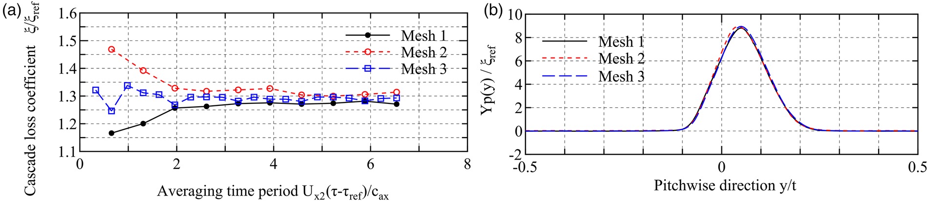
Figure 3 shows statistical and mesh convergence behaviours, which are evaluated by the pitchwise loss distribution and the cascade loss. The statistical convergence can be confirmed by the history of cascade loss shown in Figure 3a, which is obtained after the initial disturbance damped. It can be seen that the averaging over 6 through flow time is sufficient for all three meshes. The relative difference of converged cascade loss among meshes is 3.4% at maximum between mesh 1 and 2, which is sufficient for this study. In addition, a comparison of loss distribution in Figure 3b shows that only small difference exists among the meshes.
Figure 3.
Convergence behaviour (Design B). (a) Statistical convergence of cascade loss. (b) Mesh convergence of Yp distribution.
Based on these assessments, the resolution of mesh 1 and averaging period of 6 through flow time are applied to all results presented in this paper.
Result and discussion
LES of the three blades are executed to obtain time averaged flowfields. After comparing LES result with the test, the observed transitional phenomena and its sensitivity are discussed in detail.
Cp distribution and location of separation
Figure 4 shows the distributions of pressure coefficients in three blades. All three blades show different acceleration and deceleration on both surfaces. The peak of Cp increases by the order A, B, and C, which is the same order with the magnitudes of the Zw in Figure 1. Looking at the deceleration parts on the suction side from the peak Cp positions toward
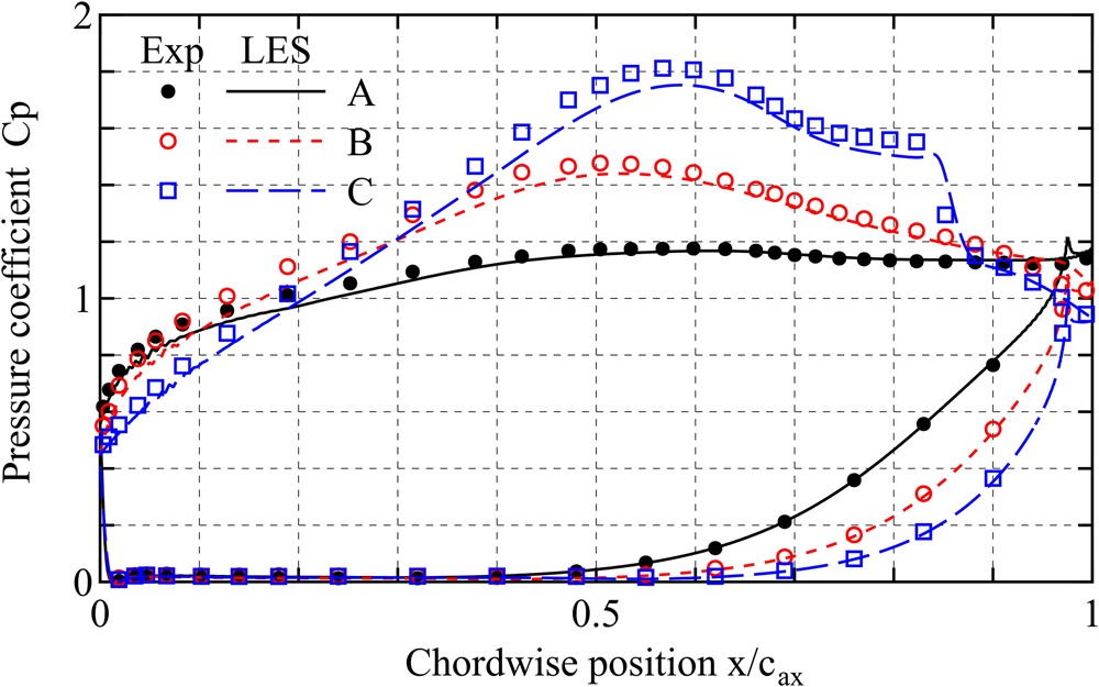
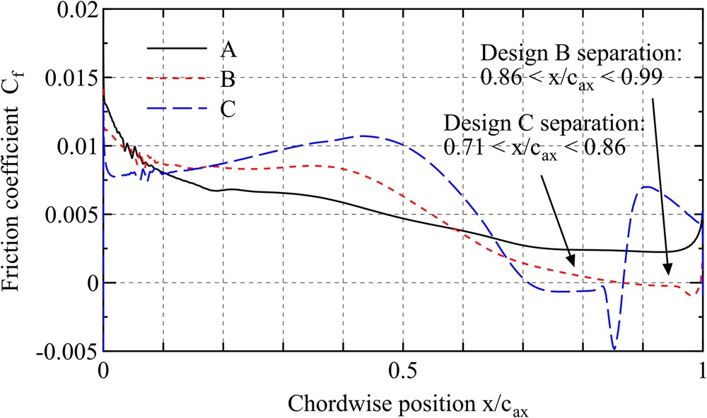
Figure 5 shows the distributions of friction coefficients Cf on the suction side, from which the occurrence of separation can be clearly observed by their negative parts. Please note that there are small wiggles near the leading edge. These wiggles are originated by non-smooth surface curvature of the blade geometry introduced during mesh generation, and does not have any harmful non-physical effects. In design C which shows clear separation induced transition in Cp, the separation occurs from 0.71 to 0.86 axial chord positions. In design B, although the existence of separation is not clear as design C, the Cf distribution clearly tells the bubble exists from 0.86 to 0.99. The reattachment occurs just on the trailing edge and the separation bubble is closed in case B. Finally, in the design A, the flow is fully attached over the blade.
Boundary layer development
In order to see whether the observed separation is consistent with the test, the boundary layer distributions are compared from 80% chord to the trailing edge. Figure 6 shows the comparisons for blade B and C. Here, the result from blade A is not presented because its boundary layer shows fully-laminar features and excellent agreement with the test. Compared to design B, the distributions in high-load design C show good agreement with the test. There is slight mismatch in
Figure 6.
Boundary layer profiles on design B and C. Design A is not shown here because the boundary layer is fully laminar on the blade, and the numerical result excellently agrees with the test. (a) Design B. (b) Design C.
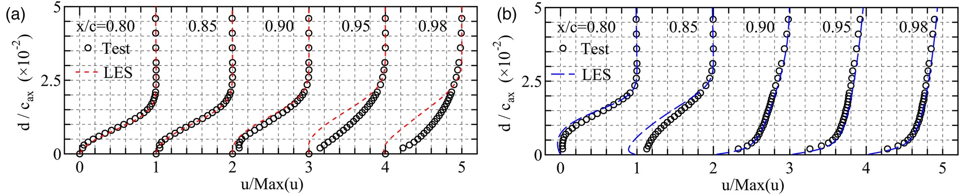
Although the design B shows good agreement until
Cascade loss characteristics
The evaluation of integrated losses is also important for design perspective. Figure 7 shows the pitchwise distributions of total pressure loss Yp for three blades. As expected from the excellent agreement in Cp and boundary layer profiles, design C shows good agreement with the test in both the height and width of the distribution.
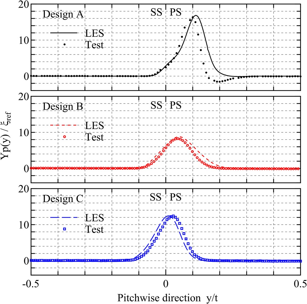
As the blade loading decreases, the prediction of loss distributions becomes worse. In design B, the distribution from LES is entirely larger than the test especially in the pressure side. Similarly, the LES result in design A also shows discrepancy in the pressure side. Although the experimental data shows negative loss, this part does not exist in LES.
Figure 8 compares the integrated cascade loss and the peak value of the loss distribution with the test results. In the integrated loss shown in Figure 8a, as expected from the previous distributions, an excellent agreement can be seen on the highest-load design C. Also, the gap between LES and test becomes worse toward the least-loaded design A.
Figure 8.
Cascade loss characteristics at STN2. (a) Cascade loss coefficients. (b) Peak of loss profile.
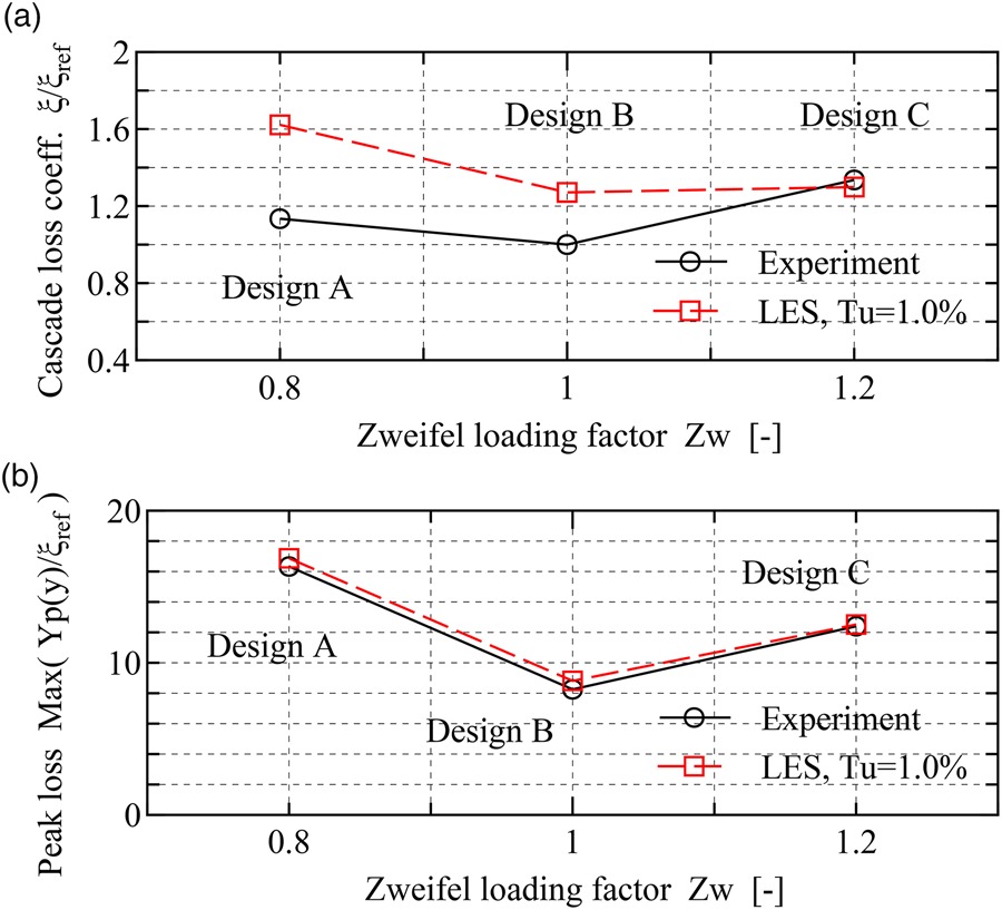
Although the total loss prediction becomes worse as the blade loading decreases, the peak of loss distribution shown in Figure 8b captures the difference in three blades quite accurately.
Instantaneous flowfields and generation of turbulent vortex structures
The flowfields and vortex structures around the cascade clearly provide the difference of unsteady flow and transitional phenomena in LPT cascades. Figures 9 and 10 show instantaneous Mach number distributions and vortex structure around the blades, respectively. The vortex structure in Figure 10 is extracted by positive iso-surfaces of Q criterion

Figure 10.
Vortex structures around the blades ( Q = 11 U 2 2 / c ax 2 )
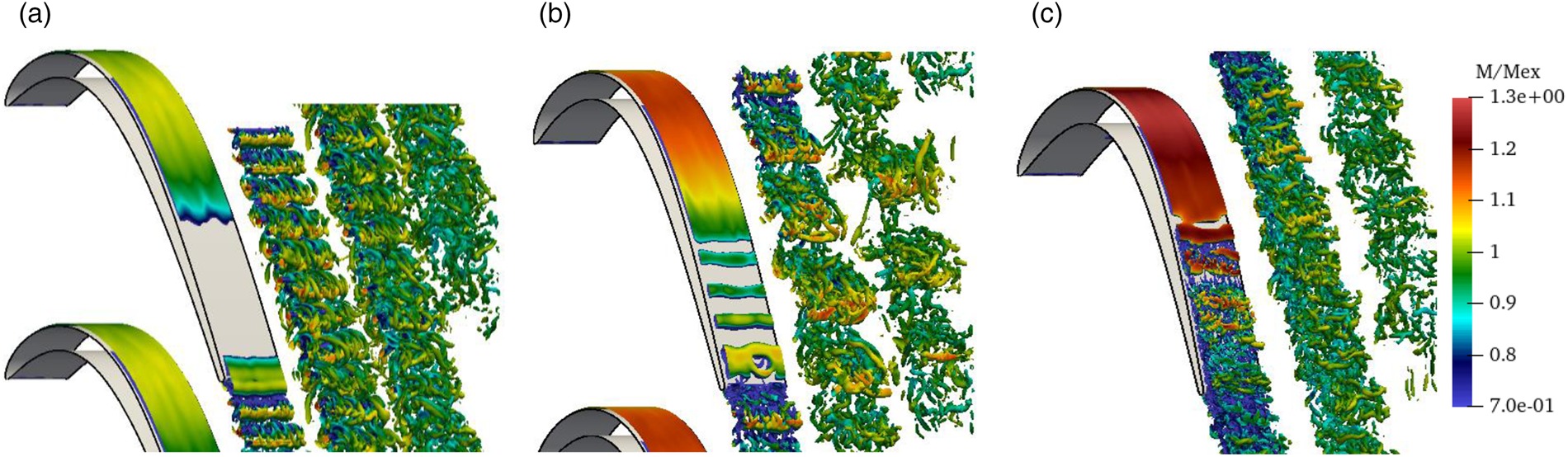
In the Mach number distribution in Figure 9, it can be seen that the development of the wake looks significantly different among the cases. There exists a wake with discrete low-speed shedding structure in design A. On the other hand, such structure cannot be seen in design C, whose boundary layer experiences transition on the suction surface due to the breakdown of laminar separation bubble. The wake in design B can be regarded as an intermediate case between A and C, where the shed low-speed structure is quickly diffused but the alternative shedding pattern can be observed clearly. These findings on the wake structures from Figure 9 are consistent with the wake pattern in Figure 10.
As well as the wakes, distinctive trends of the boundary layer can be observed from Figure 10. There are long streaky spanwise variations of Mach number due to inflow turbulence, which exist on the suction side. In the design B and C, the two-dimensional rollers can be observed on the suction side. This roller seems to be generated from the separated shear layer and quickly breaks up in design C, which is typical for separation induced transition in low-pressure turbines. In design B the rollers appear to be emerged from unstable inflectional boundary layer, and three-dimensional structures triggering transition appears just near the trailing edge. Contrary to them, design A shows no such roller structures on the blade surface.
Overall discussion of comparison with the test
Through comparisons to the experimental data and observation of the flowfields, the ability of the LES prediction for each design is summarised here. First of all, it is notable that the result of design C shows excellent agreement both in the boundary layer and loss distribution both in quantitative sense. The reason for this success is thought of as the transition of laminar separation bubble occurs very strongly compared to the design B.
Slight mismatch in the peak Cp
The acceleration around the leading edge and the peak of Cp are under-predicted in common with the three cases. These discrepancies might come from multiple reasons such as the difference in Mach number, slight mismatch in incidence angles, and streamline contraction due to secondary flows.
“Negative loss” in the wake in design A
In design A, the Cp and boundary layer distributions are successfully predicted. However, the “negative loss” in the wake, and hence the magnitude of integrated loss, is not reproduced appropriately.
The underlying mechanism of “negative loss” in the wake can be understood as energy separation in a vortex street called Eckert-Weise effect reported by Kurosaka et al. (1987). Due to the Eckert-Weise effect, the total pressure and temperature can be transferred by the two-dimensional shed vortex from the centre to the edge of the wake. Kurosaka et al also reported that the amount of energy separation was affected by the excited acoustic mode pattern of the test facility which alters the pattern of vortex shedding.
Therefore, two reasons can exist for the discrepancy in negative loss. First, the strength and two-dimensionality of vortex shedding in the present LES might be too weak compared to the test. In this case, the test-rig-specific acoustic environment should be modelled in LES. Second, the transition to three-dimensional flow of the shed vortices might occur too far upstream. The sensitivity of various conditions on the transition of wake should be investigated. Indeed, although it is not shown in the paper, stronger 2D vortex shedding and negative loss appears in both purely two-dimensional laminar calculation and unsteady simulation with dissipative upwind-biased scheme.
Delay of boundary layer transition in design B
Finally, the LES result of design B shows significantly later transition than the test. In the present LES the spanwise distance is quite short compared to the experiment, and its sensitivity should be investigated. Also, various efforts would be needed to match the peak Cp, in order to simulate the pressure gradient more accurately.
Nevertheless, the present result captures global tendencies of blade loadings, boundary layer, and loss characteristics for the three blades. The excellent matching of the height of the loss distributions in Figure 8b is quite encouraging for the future use of LES in design practice.
Effect of inflow turbulence and numerical setup
Since the mismatch between LES and test results are related to transitional phenomena, the sensitivity of inflow turbulence is evaluated as a first step of the improvement of LES prediction. Figure 11a summarizes the effect of inflow turbulence intensity on the cascade loss and peak of Yp distributions. The over-prediction of cascade losses in design B and C is not improved by elevated or depressed turbulence intensity from 1.0%. This is also the case with peak of Yp, where the results of Tu = 1.0% show the best agreement with the test.
Figure 11.
Effect of turbulence intensity on total pressure loss characteristics. (a) Peak of loss profiles for three blades. (b) loss profiles in design A.

Effect of turbulence intensity in fully-laminar blade A
Although the free stream turbulence has low sensitivity on the integrated loss, it greatly affects the loss distributions in design A. The loss distributions in Figure 11b show that the peaks are gradually diffused from 0.0% to 3.0%. In addition, the negative loss is not reproduced even under Tu = 0.0%.
In order to see the location of transition, the distributions of turbulence kinetic energy are shown in Figure 12 with focus on the region downstream of the trailing edge. There is almost no turbulence upstream the trailing edge, which indicates that the boundary layer is fully laminar even under elevated turbulence of Tu = 3.0%. Then, strong transition takes place at the base region (i.e., immediately downstream the trailing edge), which is observed in common with all the cases. Also, it can be seen that the higher free stream turbulence level greatly enhances the diffusion of the high TKE area in the wake.
Figure 12.
Turbulence kinetic energy in the wake. Thin solid line shows STN2. (a) Tu = 0, (b) Tu = 1.0%, and (c) Tu = 3.0%.
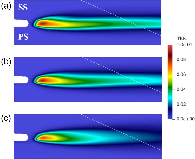
From this sensitivity study, it can be concluded that the reason for the mismatch in design A is not due to the free stream turbulence and other reasons might be exist, such as the rig-specific acoustic environment.
Sensitivity of turbulence length scale and AVDR in transitional blade B
In order to improve the location of transition, the effect of the turbulence length scale and the axial velocity density ratio (AVDR) are sequentially investigated. Here, the spanwise width is doubled (i.e.,
In order to see the sensitivity on the boundary layer transition, the AVDR is chosen to 0.96 to match the Cp distribution to the test data. The non-unity AVDR is considered by introducing additional source terms (Giles, 1991; Bolinches-Gisbert et al., 2020).
Figure 13 shows Cp, Cf, and boundary layer profiles for three length-scales, and the combination of
Figure 13.
Effect of of turbulence length scale and AVDR in design B (Tu = 1.0%). (a) Cp distributions. (b) Cf distributions. (c) BL profiles.

The flow phenomenon occurring during the migration of transition point is illustrated by the vortex structure in Figure 14. Figure 14a corresponds to
Figure 14.
Difference of the transitional behaviour for the different computational setups in design B. (a) l/cax = 0.05, AVDR = 1, (b) l/cax = 0.1, AVDR = 1, (c) l/cax = 0.1, AVDR = 0.96, ( Q = 11 U 2 2 / C ax 2 )
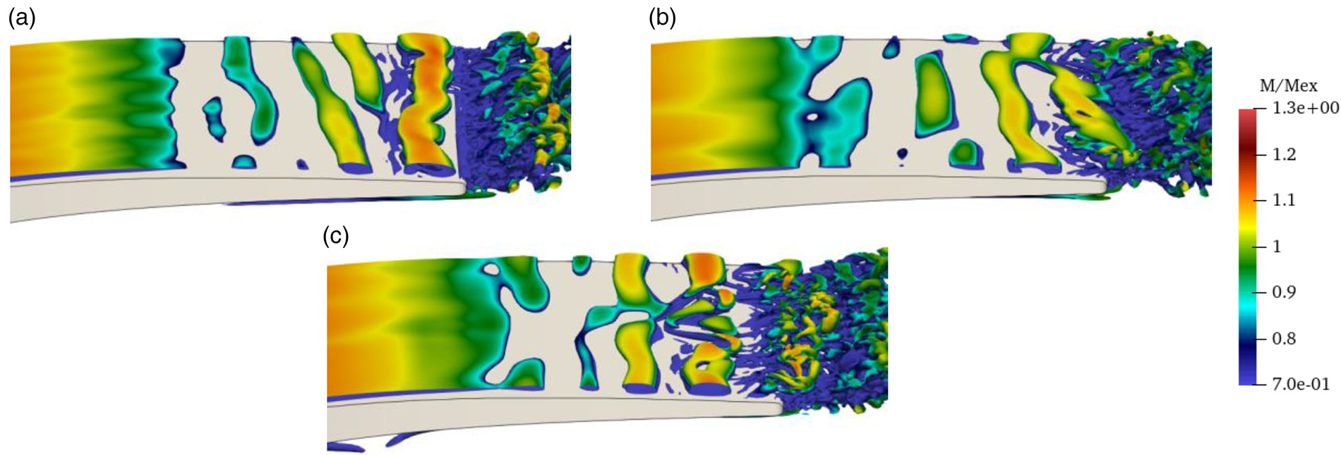
Compared to the vortex structure between Figure 14a, it can be seen from Figure 14b that transition of two-dimensional roller partly occurs near the trailing edge. The width of streaks upstream the roller is certainly affected by the scale of free stream turbulence, which yields earlier reattachment. The modification of AVDR further pushes the transition point upstream, which can be confirmed from Figure 14c. As observed here, the state of two-dimensional rollers and the transition position is highly affected by the inflow turbulence and AVDR. To summarize the sensitivity study for design B, great cares needs to be taken for a successful prediction to match inflow turbulence length scale and pressure gradient in the targeted test rig.
Conclusions
Towards future application of LES in turbomachinery design, a validation of a high-order structured overset LES code PT3D was conducted over three LPT blades with different loading and onset of laminar-turbulence transition. Through the comparison between the LES and test results, the degree of agreement and reasons of discrepancy were discussed. Then the sensitivity of inflow turbulence and numerical setups were evaluated to further improve the prediction. The findings are summarized as follows.
The prediction of the high-load blade C was satisfactory, because transition was strongly initiated by the corruption of distinct laminar separation bubble.
For the fully-laminar blade A, although the boundary layer on the blade was predicted accurately, the “negative loss” known as Eckert-Weise effect was not reproduced at all. Even under zero free stream turbulence, there was no difference in transition location of the wake, and the negative loss did not appear. In order to reproduce this phenomenon, the acoustic effect of the rig which affects the vortex shedding might be needed in the simulation.
The moderate-load blade B showed a significantly delayed transition compared to the test. The state of two-dimensional rollers and transition location were sensitive on the length scale and inflow turbulence. Also, transition location is affected by slight modification of Cp distribution by changing the AVDR.
Nomenclature
flow angle (rad)
mesh width (−)
solidity
time (sec)
viscous friction stress on the wall (Pa)
axial velocity density ratio (−)
axial chord length (m)
friction and pressure coefficients (−)
wall-normal direction (m)
spanwise height of the streamtube (m)
eddy size in synthetic eddy method (m)
local Mach number, isentropic exit Mach number (−)
total and static pressure (Pa)
Q-criterion (1/sec2)
pitch length (m)
turbulence intensity (−)
axial velocity (m/s)
axial direction (m)
pitchwise direction (m)
spanwise direction (m)
local total pressure loss coefficient (−)
Zweifel’s loading factor (−)
cascade loss coefficient (−)