Introduction
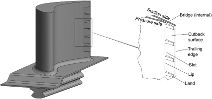
In the modern gas turbine engines of today, the high-pressure turbine (HPT) blades are exposed to harsh aerothermal environments, with the temperatures of the working fluid in excess of the metal melting point temperature. The need for effective cooling of the metal surface is crucial to maintaining the component life as well as the safe operation of the engine. One such area of cooling that is a challenge is the trailing-edge slot (also known as the pressure-side bleed), as shown in Figure 1. The aerodynamic requirements dictate the trailing-edge be tapered to increase the aerodynamic efficiency, which prevents internal cooling solutions. Instead, the cooling is provided by injecting the coolant fluid out of the slot, forming a film on the metal cutback surface. The interaction of this film with the extraneous working fluid leads to interesting flow dynamics, producing either wall-jet or wall-wake type flows. The flow physics for the trailing-edge slot has received attention both experimentally (Kacker and Whitelaw, 1969, 1971) and numerically (Medic and Durbin, 2005; Joo and Durbin, 2009; Haghiri and Sandberg, 2020) in order to understand how effective the slot fluid is in shielding the metal surface, quantified by a non-dimensional adiabatic wall effectiveness η
Figure 1.
where Tw,Tfs and Ts represent the adiabatic wall, freestream and slot fluid temperatures, respectively. Lower values of η indicate higher wall temperatures, on account of the negative denominator in Equation 1. From a design perspective, predicting these wall temperatures numerically is fraught with challenges, stemming from either the excessive cost of high-fidelity simulations or unacceptable inaccuracies from low-fidelity tools like Reynolds-Averaged Navier-Stokes (RANS) (Launder and Rodi, 1983; Holloway et al., 2002a) or unsteady RANS (URANS) (Holloway et al., 2002b; Ivanova and Laskowski, 2014). The poor prediction of η for these flows when using RANS-based closures is attributed to the incorrect momentum and thermal mixing modelled, which ties into the closures for the turbulence stress (Boussinesq approximation) and turbulent heat-flux (gradient diffusion hypothesis). With the availability of high-fidelity data for these flows, building better models of the closures for the stress and the heat-flux through machine-learning approaches is gaining increasing attention. In a RANS context, studies such as Sandberg et al. (2018) and Haghiri and Sandberg (2020) developed closures for the turbulent heat-flux by fixing the velocity field from high-fidelity data while the URANS closures in the studies of Lav et al. (2019a) and Lav and Sandberg (2020) were developed for both the turbulence stress tensor and the heat-flux vector. These studies obtained the closures with the aid of a genetic evolutionary algorithm, the gene-expression programming for RANS (Weatheritt and Sandberg, 2016) and for URANS (Lav et al., 2019b). This machine-learning algorithm performs symbolic regression to obtain a mathematical expression that attempts to match the reference quantity of interest, obtained from high-fidelity data, and thus far has been used to develop expressions for the turbulence stress tensor (via tensorial regression) and the turbulent heat-flux vector (via scalar regression). It is noteworthy that the expressions are obtained by regressing against the high-fidelity quantity of interest, leaving the utilisation of RANS or URANS out of the closure development process, also known as “training”. While gene-expression programming (GEP) in the present form leads to quick closure development times (of the order of minutes), one crucial issue with this approach is the lack of any information related to the velocity or temperature fields during the closure development process. Implementing these closures into RANS/URANS solvers a posteriori has shown to improve the flow prediction remarkably over the commonly used closures but improvement of the turbulent stress tensor or heat flux vector prediction does not always lead to equally improved mean flow predictions. In that vein, the GEP algorithm was modified by Zhao et al. (2020) to include contributions of the velocity field into the closure development process to build more robust turbulence stress closures for high-pressure and low-pressure turbine wake flow predictions. This was achieved by running RANS calculations within a loop during the algorithm's execution to develop turbulence stress closures that improved the flow prediction instead of just the turbulence stress. The modification of the algorithm in this way was labelled as CFD-driven machine learning (or “looped” training) while the conventional use of the GEP is denoted as data-driven machine-learning (or “frozen” training).
Thus, in the present study the CFD-driven machine learning approach of Zhao et al. (2020) is adapted to develop closures for the turbulent heat-flux, where RANS calculations for the temperature field are incorporated into the training and used as a target for improvement. High-fidelity datasets of three blowing ratios for a given lip thickness geometry from Haghiri and Sandberg (2020) are used to lead the model development and the closures obtained from this looped training are compared with the high-fidelity data, the conventional frozen trained closures in addition to the commonly used gradient diffusion hypothesis closure.
Numerical setup
Reference datasets
The highly-resolved large eddy simulation (LES) datasets of a fundamental trailing edge slot, performed by Haghiri and Sandberg (2020), are used in the present study as the reference for sake of model development. The data was produced using an in-house multi-block structured compressible Navier–Stokes solver HiPSTAR (Sandberg, 2015). Figure 2 shows a schematic of the flow configuration. At the inlet boundary, a cold wall jet and a plane hot co-flow with different speeds are specified, separated by a flat plate with thickness t. The inlet mean velocity profiles were adapted from the experimental study of Whitelaw and Kacker (1963). In the LES, only mean profiles were prescribed at the inlet boundary and no fluctuations were added. All walls were set to no-slip boundaries and adiabatic temperature conditions were used. The wall adapting local eddy viscosity (WALE) model (Nicoud and Ducros, 1999) was used for modelling of the sub-grid scale stresses. Table 1 summarises the details of the three cases. Interested readers can refer to the original paper of Haghiri and Sandberg (2020) for more details on the flow configuration and numerical setup.
Figure 2.
Computational domain (not to scale). The structures shown represent contours of the Q-criterion, coloured by the temperature field in the range [0.85, 1.0], non-dimensionalised by the freestream temperature.
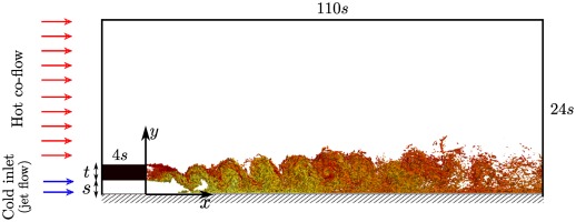
Table 1.
Simulation parameters.
| CASE | t/s | BR | Reslot | Ufs (m/s) | Tslot (K) | Tfs(K) |
|---|
| A1 | 1.14 | 1.26 | ≈12,000 | 19.2 | 273 | 323 |
| A2 | 1.14 | 1.07 | ≈10,000 | 19.2 | 273 | 323 |
| A3 | 1.14 | 0.86 | ≈8,000 | 19.2 | 273 | 323 |
RANS-based scalar flux closures
Even with the recent rise of computational power, LES is prohibitively restrictive within an industrial design context, ensuring that the dependence on RANS continues. Unfortunately, RANS is known to suffer from two major sources of modelling errors: Reynolds stress and turbulent heat-flux closures. In the present study, the focus is placed only on the latter and it is assumed that the momentum field (velocity) and other inputs to heat-flux models are known accurately (from time-averaged LES in this case). The mean temperature transport equation for an incompressible flow is given (in non-dimensional form) below:
where
In the above, xi and t are the spatial coordinate vector and time, respectively. In addition, ui is the velocity vector, T is the temperature, Re is the Reynolds number and Pr is the Prandtl number. It should also be noted that “asterisk” and “overbar” represent dimensional and time-averaged variables, respectively. The use of the incompressible framework here is justified due to the low Mach number (<0.3) in the freestream and the jet flows. Furthermore, the buoyancy effects are negligible due to the small temperature differences between the freestream and the jet flows, implying that the energy equation can be decoupled from the momentum equations (Sandberg et al., 2018). As such, the temperature field can be solved passively.
The turbulent heat-flux is commonly modelled using the gradient diffusion hypothesis (GDH), assuming that the heat-flux terms are in the direction of their corresponding maximum mean temperature gradient
where the diffusivity αt=νt/Prt is modelled as eddy viscosity (νt) over turbulent Prandtl number (Prt). The eddy viscosity concept is commonly used in closures of Reynolds stress tensor while the turbulent Prandtl number is assumed to be constant, with Prt=0.9 widely used in the literature. The GDH implies that the turbulence isotropically diffuses the heat, which is known not to be the case, except perhaps for simple free shear flows (Fabris, 1979). There are indeed more accurate approximations to model the turbulent heat-flux vector, such as the Generalised Gradient Diffusion Hypothesis (Daly and Harlow, 1970) or the Higher Order Generalised Gradient Diffusion Hypothesis (Abe and Suga, 2001) which have been explored previously (Ling et al., 2015; Weatheritt et al., 2020). However, in this study the closures are exclusively developed for the GDH for two main reasons. First, the simplicity of the GDH closure can not be discounted, which helps in running stable calculations in the RANS solver. Second, the GDH closure developed in this study using the CFD-driven approach can serve as a direct comparison with the GDH trained closure obtained from the frozen approach in Haghiri and Sandberg (2020). Consequently, it offers the chance to evaluate whether further improvements using the GDH can be obtained in prediction of η when switching to a CFD-driven training approach. Thus, in the present study, the constancy of Prt in Equation 4 is upended in lieu of a scalar functional form obtained as a function of velocity and temperature gradients using the symbolic regression-based machine learning framework outlined below.
The machine-learning framework
To perform the optimisation in the present study, we use gene-expression programming (GEP), which is a symbolic regression algorithm returning mathematical equations (Ferreira, 2001). The biggest advantage of using GEP over other algorithms is the portability and transparency of returning an equation, allowing for inspection of the generated terms and interpretation of the optimisation outputs. In GEP (drawing an analogy with Darwin's survival-of-the-fittest theory), an initial population of candidate solutions is randomly generated at generation step i=0. From this pool of candidate solutions, the fitness of each candidate is evaluated based on a cost function. Subsequently, selection (survival-of-the-fittest) directs the search away from poorer candidates and weights the chance of survival towards fitter functional forms. This is achieved through tournament selection, whereby the candidate solutions compete with each other to survive based on their fitness. The genetic operators then (e.g. mutation, crossover) provide the search aspect of the algorithm, applying variations to the existing solutions, updating the population of candidate solutions at the next generation i+1. The search then iteratively continues through several generations until a functional form that “best” fits the dataset (the optimum solution) is obtained. The functional form returned by the algorithm depends on the random initialisation when generating the population of candidate solutions at generation i=0, i.e. it is a non-deterministic process. However, the fitness of the functional forms have been observed to be not too dissimilar, leading to similar performances when the closures are tested a priori and a posteriori (Haghiri and Sandberg, 2020). Interested readers can refer to Koza (1994) and Ferreira (2001) for introductory information of the GEP algorithm, whereas the details of using GEP in turbulence modelling was specified in detail in Weatheritt and Sandberg (2016).
Frozen training process
The data-driven closure for the turbulent heat-flux in the frozen approach is developed by adopting the gradient-diffusion hypothesis by minimising the cost function
which is the mean-squared error of Equation 4 where αt=αgepνt. Note that V represents the points within the training region. The training region refers to the spatial extent of the domain from where the data points are picked to undergo the training. Therefore, the target for optimisation is a non-dimensional parameter αgep, which can be seen as the inverse of a non-constant turbulent Prandtl number with a functional dependence on the velocity and temperature gradients,
where, considering the present statistically two-dimensional flow, the function αgep is formed by constructing independent invariants from sij=Sij/ω, wij=Ωij/ω, and ϑi=k/β∗ω(∂T¯/∂xi) given as follows:
The invariants used in this study represent an integrity basis (Smith, 1965) to ensure the coefficient αgep remains Galilean invariant. Owing to the statistically two-dimensional nature of the flow, Equation 7 represents a subset from the full list of invariants as listed in Milani et al. (2018) and discussed in Pope (1975). In Equations 5 and 6 the turbulence eddy viscosity (νt) and the specific turbulence dissipation (ω) are, respectively, needed in the data-driven solutions. As such, νt and ω are obtained through a frozen approach in which the “true” (high-fidelity) velocity and Reynolds stress is held constant and only the ω transport equation is solved, resulting in νt=k/ω consistent with both the high-fidelity database used and the turbulence model equations. Hence, apart from the frozen approach to obtain νt, there is no CFD involved in the machine learning process here. A detailed investigation by Haghiri and Sandberg (2020) on different BRs and lip thicknesses found that the turbulent heat-flux closure developed for the thickest lip (t/s=1.14) and the highest BR of 1.26 performed extremely well on itself, other flow conditions and lip thicknesses. Thus, in this paper, we consider the BR = 1.26 case for comparison and closure development. The developed machine-learnt heat-flux closure (αtmod=αgepνt) generated with the above described framework, using the LES case of BR = 1.26, is given as follows
A box domain training region was chosen for developing this closure, where the wall normal extent ranged from 0≤y≤3 and the streamwise extent covered 30≤x≤85. The functional form obtained here constitutes the “Frozen” model and will be used later on to compare the new closures developed via the looped training approach, described next.
Looped training process
The looped training process discussed here is an adaptation of the method described in Zhao et al. (2020), extended to scalar regression. While the cost function in the previous section was obtained by computing the error difference between the reference and model heat-fluxes, the cost function evaluation here is performed by running RANS calculations in the loop to obtain the difference between the reference and the model. A key advantage of running RANS in the loop is the ability to modify the quantity used to evaluate the cost function. Thus, the looped training process can be used to find a turbulent heat-flux closure that improves the temperature field, instead of the turbulent heat-flux as was considered in the frozen training process. An example of the cost function used here is given by
T¯ref is obtained from a reference dataset while
T¯gep is obtained after a RANS is run with a heat-flux closure from GEP. The RANS runs the scalar transport equation (Equation
2) for the temperature field, using the velocity field and
νt (obtained from the frozen procedure) from the reference time-averaged LES data. The temperatures in Equation
9 could be from any spatial location, using the whole domain or select spatial positions. The latter is advantageous when the reference dataset is limited, as is often the case in experiments. The GEP algorithm produces a candidate pool of models for the heat-flux, generated randomly, which are used to run RANS calculations. Upon reaching a converged RANS solution, a cost function is evaluated (like in Equation
9) and the error returned back to the algorithm. Based on the models with the lowest returned errors, a new pool of models is generated using the evolution principles also used in the frozen training. These new models are evaluated again by running RANS calculations and the cycle repeats until the best surviving model remains, based on some stopping criterion such as the number of generations or an error threshold. This approach should generally lead to better closures compared to the frozen training because it implicitly includes the effect of other modelling errors present when solving the RANS equations. The RANS calculations are performed with OpenFOAM v2.4 which interfaces with the GEP algorithm. The scalarTransportFoam solver is modified to read the GEP-generated model form as a wordList string which the algorithm pipes to a file in a given generation. This string is used to construct the scalar expression in Equation
6 and thus solve Equation
2. At the end of the converged run, the RANS result is sampled at the spatial locations of interest and an error value using Equation
9 is evaluated. If the RANS fails to converge, the error is set to a very large number to automatically filter out unstable models. The difference between the two training approaches is summarised in
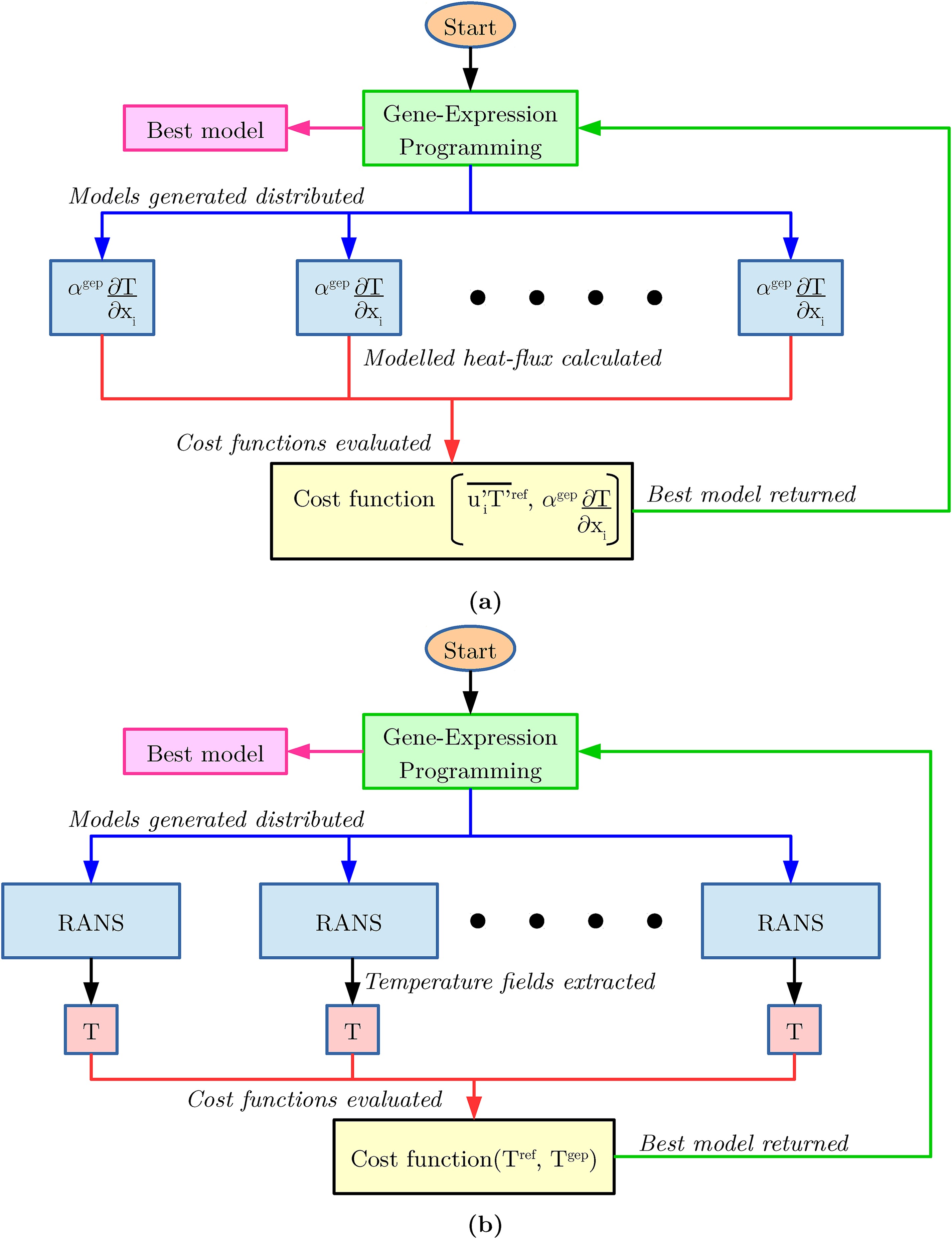
Figure 3 via a schematic.
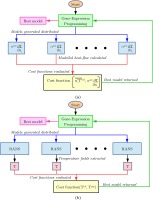
Figure 3.
Schematic of the (a) frozen and (b) looped training process.
Results and discussion
Grid independence
Since the looped training relies on running multiple RANS calculations simulataneously and iteratively, the runtime of these RANS can require large computational resources and dramatically increase the model development time. Thus, it is crucial to have as cheap a RANS setup as possible for the training. This is attained by coarsening the grid resolution without compromising the solution accuracy. A grid independence test is performed on the frozen GEP trained case (referred to as “Frozen”), i.e. with αt given by Equation 8 in OpenFOAM v2.4. The temperature equation was solved using a smoothSolver with the GaussSeidel smoother and a tolerance of 10−16. A relaxation factor of 0.7 was used on the temperature equation as well as the final temperature at each iteration. The discretisation schemes used for the gradient, divergence, laplacian and interpolation operators were Gauss linear, bounded Gauss linearUpwind grad(T), Gauss linear corrected and linear respectively.
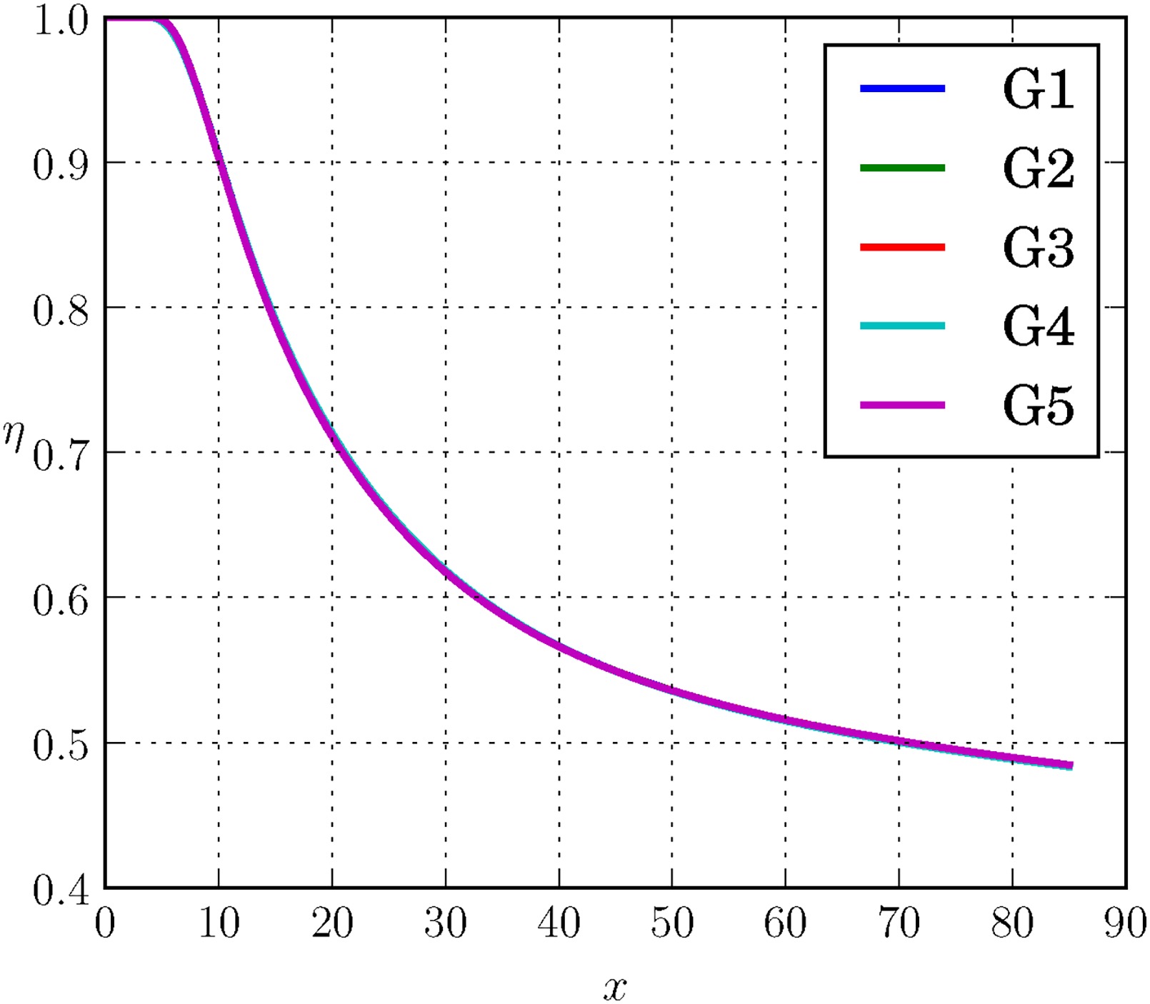
Figure 4 shows the adiabatic wall effectiveness η for the BR = 1.26 case tested on multiple grid resolutions while Table 2 shows the details of the grid resolutions tested. The results indicate that the coarsest grid tested, i.e. G5, shows excellent agreement with the reference LES grid G1 for the frozen case. With a runtime of ∼15 s running on a single core laptop, grid G5 is ideally placed to conduct the looped training. Additionally, the cost of the training process can be further minimised by executing the GEP algorithm for a smaller number of generations, chosen to be 100 here, running 4 RANS calculations per generation (representing the tournament size) followed by 20 mating operations per generation, resulting in a total model development time of approximately 4 h. This means that at any given generation, 4×20=80 candidate solutions are being evaluated before proceeding to the next generation. It will be shown later that even with a reduced number of generations, the closures that improve the prediction can still be obtained. The number of RANS in the loop was chosen such that it matches the number of cores on the compute node. In contrast, the frozen training had been conducted for 3,000 generations, with 2 tournaments per generation followed by 50 mating operations per generation (i.e. 2×50=100 candidate solution evaluations per generation), which took about 20 min. It must be pointed out that the purpose of the looped training process here is to demonstrate the effect of including RANS calculations in the optimisation process, rather than finding the best parameters to run the GEP algorithm. As a rule of thumb, increasing the number of generations, which represents the iterations, leads to a model with better fitness values. Consequently, a longer looped run was also conducted on a larger compute node with 12 cores for 400 generations, running 12 RANS calculations per generation followed by 50 mutation operations per generation, bringing the total model creation cost to approximately 30 h.
Figure 4.
Grid convergence test on grids from Table 2 using the frozen closure from Equation 8 on BR = 1.26 case.

Table 2.
Grid independence study.
| Grid Caption | Nx×Ny | Processors | Runtime (s) |
|---|
| G1 | 1681×386 | 24 | 750 |
| G2 | 841×194 | 12 | 150 |
| G3 | 421×98 | 6 | 50 |
| G4 | 211×50 | 3 | 20 |
| G5 | 106×26 | 1 | 15 |
Effect of cost function
With the availability of RANS calculations within the looped training process, a clear advantage over the frozen training is the ability to choose any quantity as a cost function to develop the closure for the heat-flux. Using the BR = 1.26 case as the reference for model development, two cost functions are tested, the temperature distribution along the wall, i.e. y=0, and the wall-normal temperature distribution at 3 streamwise locations, i.e. x=10,30 and 50. The resulting closures obtained are given by
where superscripts
ST and
WT refer to the closures developed using the streamwise temperature profiles and wall temperature as cost functions, respectively. Compared with Equation
8, the looped closures in Equations
10 and
11 are simpler in form and have larger values of the constants within the expression. The simpler expression forms are a feature of the looped training process and was first discussed in
Zhao et al. (2020) for the turbulence stress closures while the high value of the constants indicate a requirement of an even lower
Prt than what the frozen trained model returned to improve the prediction. Interestingly, the contribution from the invariants in Equations
10 and
11 relative to the constant term were found to be smaller in magnitude, indicating that the major contribution to the turbulent heat-flux comes from the constant term. The prediction of
η and the temperature profiles using these closures are presented in
Figure 5. The predictions from calculations of the baseline and the frozen models are also added to the figure to highlight the effect of incorporating RANS into the data-driven model development process.
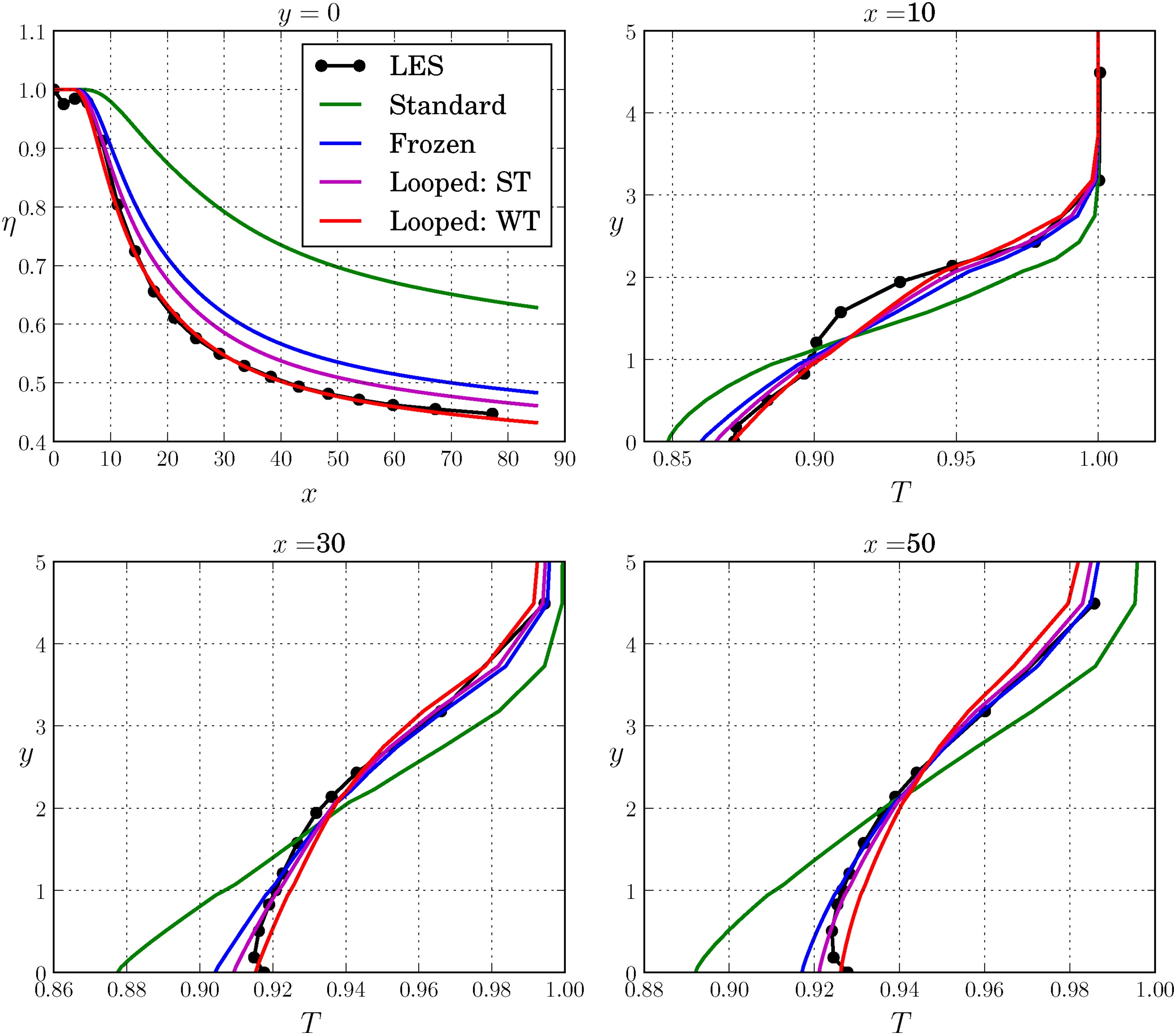
Figure 5.
Comparison of predictions from standard, frozen and looped closures with LES data, trained and tested on the BR = 1.26 case.
It is evident from the figure that looped training leads to an improvement over frozen training using both cost functions. The use of the streamwise temperature profiles as a cost function improves the temperature prediction everywhere except for points near the wall. The wall temperature cost function performs better for points near the wall, leading to an excellent match with the η profile, however compromising the streamwise temperature profile prediction for y∈[0.5,2]. Given the excellent agreement in η using the WT closure, the next sections will use this particular cost function for any subsequent model development.
Generalisability
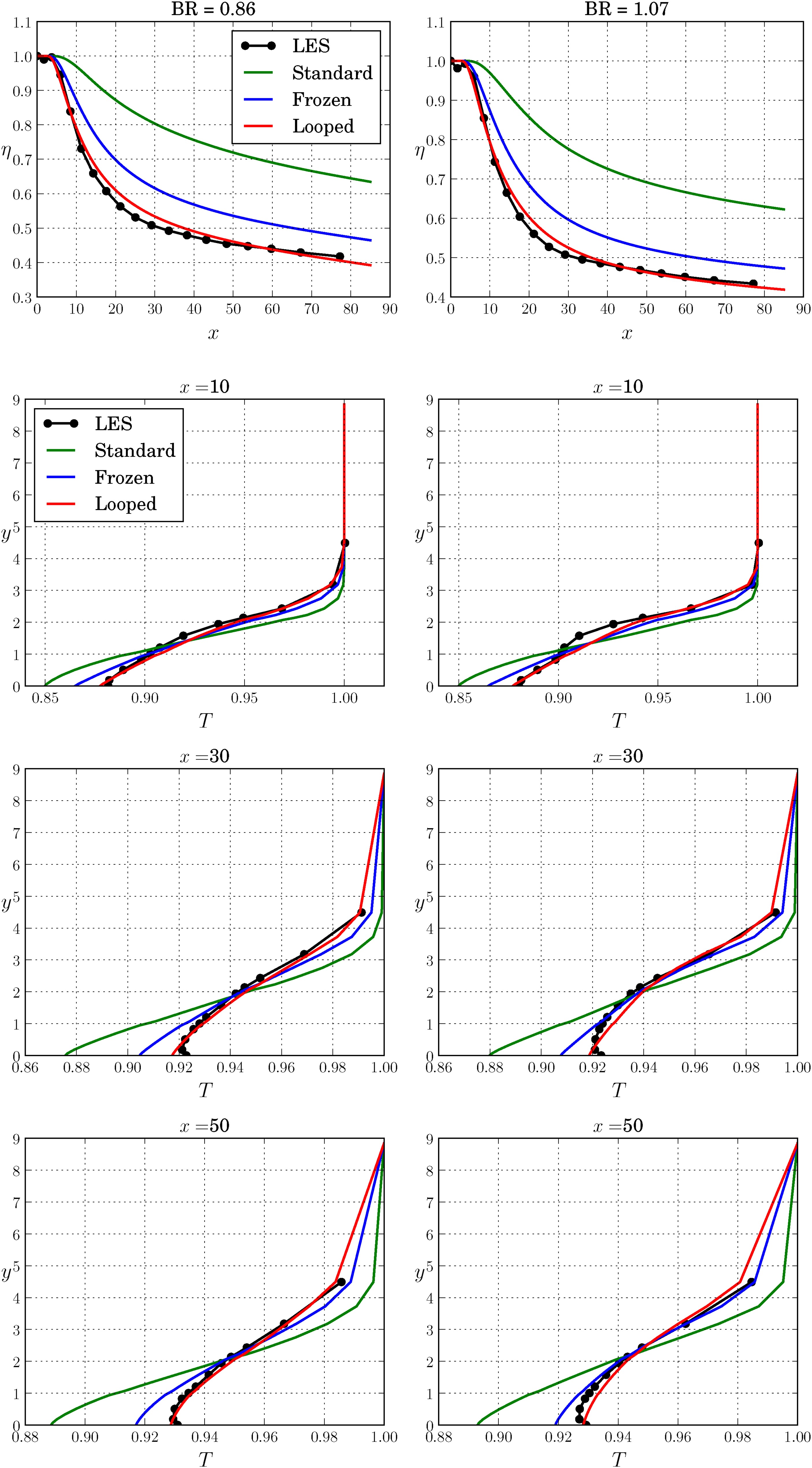
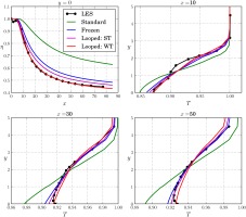
Based on the excellent improvements obtained with the wall temperature closure (Equation 11) for the BR = 1.26 case, its potential is also tested on separate flow conditions to evaluate its generalisability. Blowing ratios of 0.86 and 1.07 are run with this closure and the η predictions are presented in Figure 6. For the sake of consistency, the BR = 1.26 frozen closure was used to test the frozen closure's generalisability across the other BRs.
Figure 6.
Comparison of predictions from standard, frozen and looped closures trained on the BR = 1.26 case and applied on the BR = 0.86 and 1.07 cases.
There is a slight overprediction in η for x∈[15,40] for BR = 0.86 and for x∈[15,35] for BR = 1.07, followed by slight underprediction beyond x=60 with the looped closure. However, the looped closure clearly performs better than the frozen closure for both the BRs. To further investigate improvements in η, a looped closure development for BR = 0.86 was conducted, first using the shorter 100 generation 4 RANS run and then using a longer 400 generation 12 RANS run, resulting in the following models:
where the superscripts
S,L correspond to the short and long runs of the looped training algorithm. The resulting
η profiles are plotted in
Figure 7 where the two models are compared with the looped BR = 1.26 closure.
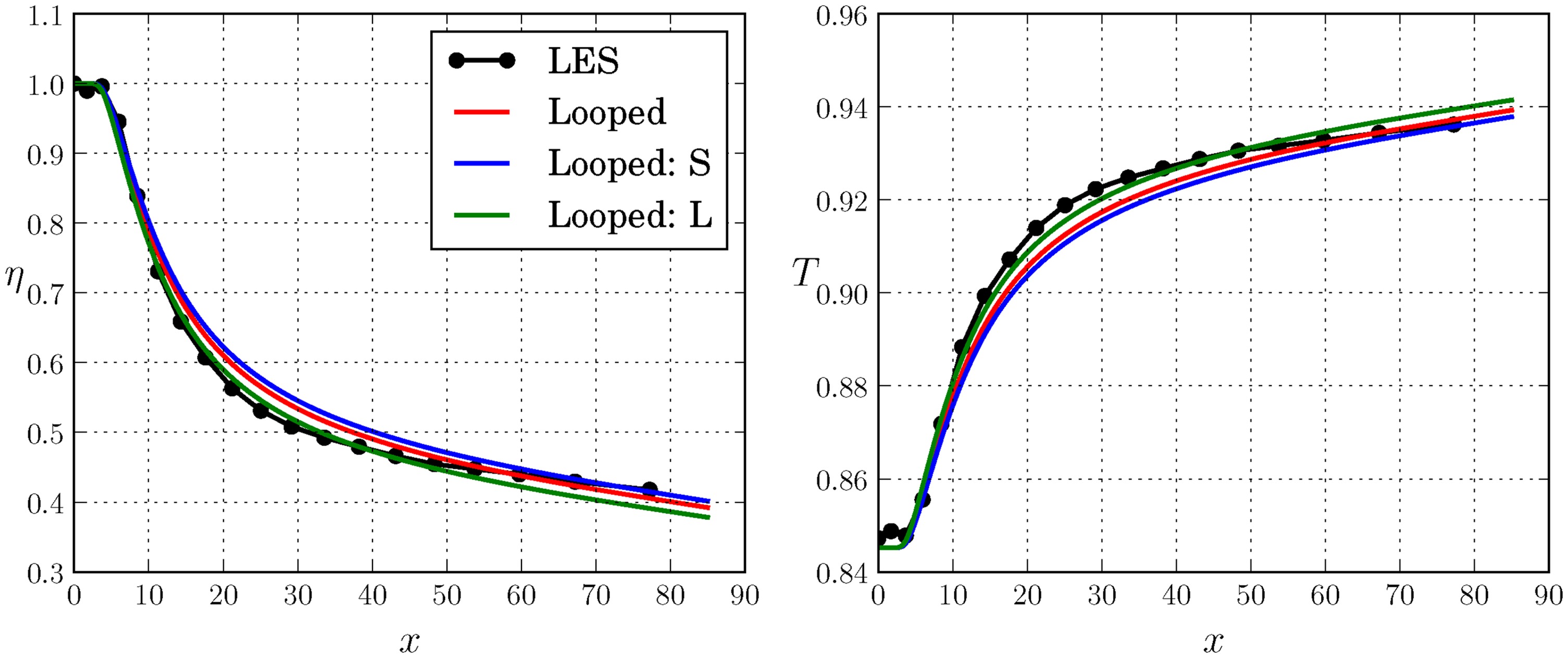
Figure 7.
Comparison of the predictions from the looped closures obtained from the BR = 1.26 case (Looped), the short (Looped: S) and the long (Looped: L) looped runs from the BR = 0.86 case, applied to the BR = 0.86 case.
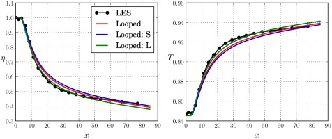
The results show that the αtS closure for BR = 0.86 (Equation 12) slightly overpredicts the η and thus performs less well than the BR = 1.26 closure (Equation 11). This is however not proof the algorithm could not find a better closure, just that it was not run for a long enough number of generations. Doing so does lead to a better prediction of η, as demonstrated by the αtL closure (Equation 13).
Multidata training
The ability of running RANS in the loop to develop a closure leads to an interesting possibility, i.e. developing closures for multiple datasets at once. A short run with 100 generations using 6 RANS per generation, with 2 RANS per BR and a long run with 400 generations using 36 RANS per generation, with 12 RANS per BR were performed with the resulting closures given by:
where the superscripts
S,MD and
L,MD correspond to the short and long multidata runs of the looped training algorithm. The cost function remains the same as Equation
9, where the
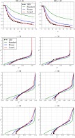
T¯ref for a given RANS run depends on the BR and is chosen accordingly. Effectively, all three BRs are made to compete simultaneously in a given generation with different candidate solutions, eventually leading to the selection of the candidate with the best fitness. The predictions with these new closures are presented in
Figure 8, where the short run (Equation
14) performs slightly worse than the looped BR = 1.26 closure (Equation
11) while the longer run closure (Equation
15) improves the prediction even further. There are locations, particularly beyond
x=40 where the long run leads to an underprediction of
η for all BRs. This directly ties into how the selection of the best model is made during the training process. Even though the training includes multiple BRs, the model with the lowest fitness across a given generation survives, which usually occurs for one BR only, in this case BR = 1.26. This leads to a bias toward a particular model during the training process geared toward one BR only. A possible rectification to this bias is part of future investigations.
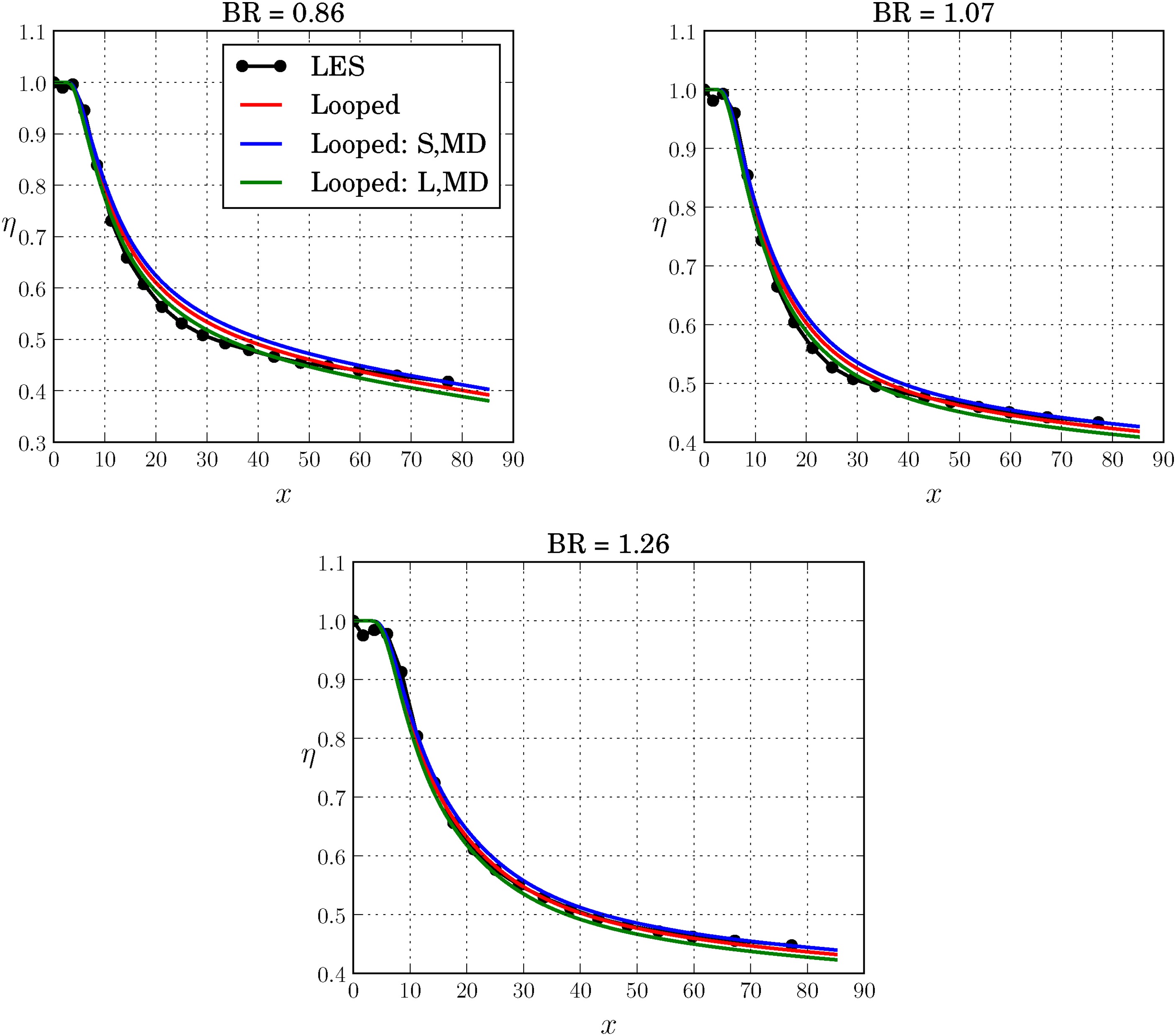
Figure 8.
Comparison of the predictions from the looped closures obtained from the BR = 1.26 case (Looped) and the short (Looped: S,MD) and long (Looped: L,MD) looped multidata runs using BR = 0.86, 1.07 and 1.26 cases, and applied on the three BRs.
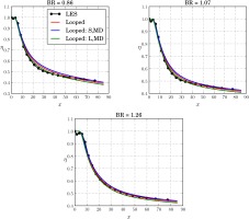
Nevertheless, the results with the looped training show that the closures developed do perform better than their counterparts from frozen training, are shorter in their mathematical extent and generalise well across other flow conditions.
Conclusions
In this study, a novel symbolic scalar regression machine-learning algorithm was applied to improve the prediction of the wall-temperature in a fundamental trailing-edge slot. The prediction of the temperature is improved by developing a scalar mathematical expression to represent a non-constant turbulent Prandtl number within the gradient diffusion hypothesis for the turbulent heat-flux. The conventional use of the machine-learning algorithm, also known as the “frozen” training process, obtained this expression by minimising the error between the true turbulent heat-flux from high-fidelity data and the model expressions generated by gene-expression programming (GEP). In the novel approach, i.e. the “looped” training process, the scalar expression is derived by conducting RANS calculations in a loop within GEP. This leads to promoting the expressions which minimise the error between the true temperature field from the high-fidelity data and the RANS solution. Thus, the closure for the turbulent heat-flux which improves the temperature field prediction can be obtained instead of the closure that improves the turbulent heat-flux prediction. This approach also allows for the use of any type of cost function and for the largest blowing ratio of 1.26, two such functions were tested, with the one based on the wall-temperature value leading to the best prediction. The resulting closure from the looped approach was also found to be mathematically succinct compared with its frozen counterpart and improved upon the prediction of the wall-temperature significantly further. The closure showed that the effective turbulent Prandtl number was required to be even smaller (∼0.32) than the frozen closure's value of 0.42 to realise improvements and generalised well upon application to the other blowing ratios. Finally, the looped approach was also demonstrated to build closures by combining datasets from multiple blowing ratios, which led to further improvements in terms of the generalisation.