Introduction
Accurate determination of the small-scale flow effects and turbulence in turbomachinery applications demands the ongoing development and improvement of experimental methods. Since access to the flow is severely limited in turbomachinery applications, the Laser-Doppler-Anemometry (LDA) has gained acceptance as a non-intrusive and unsteady single-point measurement method. In contrast, the Hot-Wire-Anemometry (HWA)—as an intrusive and unsteady single-point measurement method—has established itself as a reliable and cost-effective measurement technique. Since the principle of the HWA is based on the forced convective heat flux and thus flow velocities are measured indirectly, the measuring technique requires calibration. LDA, on the other hand, requires no calibration in principle, provided that the intersection angles of the beams are known exactly. The LDA is affected by several uncertainties due, for example, to the optical setup, probe alignment or response of the tracer particles to flow fluctuations. The HWA also exhibits measurement uncertainties, e.g., due to its intrusive nature, thermal damping effects along the measuring wire, and calibration. In this context, Ramond and Millan (2000) compared one-dimensional LDA measurements with HWA measurements in the turbulent wake of a blade profile. Here, the gradient bias was identified as one of the notable measuring errors of the LDA, which led to an overestimation of the velocity fluctuations in turbulent flows (cf. also Zhang (2002)). Zhang and Eisele (1998) have argued, that fringe distortion resulted in an overestimation of the degree of turbulence. According to them, however, this systematic measurement uncertainty only has a significant impact at low turbulence intensity flows. For the HWA, Morris and Foss’s (2003) numerical investigations showed that thermal transient effects along the hot wire can lead to the actual velocity being underestimated in flows with high turbulence intensities. This effect is enhanced by the spatial averaging of the turbulent fluctuation components along the hot-wire. Ligrani and Bradshaw’s (1987b) investigations indicated a correlation between time-averaged turbulence intensity and the dimensions of the measuring wire. By comparing HWA probes with varying wire diameters d and lengths l, they were able to show how the spatial resolution and frequency response change depending on different wire geometries. Hutchins et al. (2009) have investigated the influence of the length-to-diameter ratio l/d at moderate Reynolds numbers. Their results showed, that a reduction of l/d below 200 has a negative effect on the measured turbulent fluctuations and affects the energy spectra of the measurement data.
This paper aims to quantify and explain three-dimensional LDA and HWA measurement deviations regarding turbulence measurements within the wake of a blade profile at moderate Mach numbers and Reynolds numbers. A wake flow is promising as a means of evaluating the two measuring techniques, since it comprises regions with and without velocity gradient. This allows the investigation of various influences, such as the effect of the different measuring volume sizes. The flow conditions are chosen to represent a typical compressor flow. Such flows are characterized by turbulence spectra that can extend to several tens of kilohertz. A non-orthogonal two-probe LDA arrangement and triple wire HWA probes with lance-head (LH) and elbow-head (EH) are considered. First, the accuracy of the three-dimensional velocity measurement by the LDA system is evaluated, focusing on the indirectly measured third velocity component. The HWA probes are then compared to a corrected LDA data set. A detailed analysis is performed on the high-frequency regions of the measured turbulence spectra and potential reasons for measurement deviations are highlighted.
Experimental setup
Round jet wind tunnel
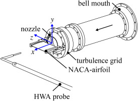
The tests were carried out at a round jet wind tunnel. The wind tunnel consists of a large settling chamber followed by a bell mouth and a round nozzle 60mm in diameter. The test stand is fed by an external air supply. To generate a turbomachine-like airfoil wake, a NACA 64A008 airfoil was mounted within the potential core of the round jet. The measuring section with the mounted wake generator is shown in Figure 1 and has been described in detail by Hölle (2019). To increase the turbulence level, a squared mesh of round bars with a diameter of 0.9mm and a mesh size of 4.5mm was placed upstream of the nozzle. Based on Roach's correlation for the turbulence intensity (Roach, 1987) and the contraction correction by Rannacher (1969), the three-dimensional turbulence intensity in the measuring plane is estimated to be Tu=2%. The operating point is defined by the isentropic Mach number M,
Figure 1.
Measuring section with horizontally mounted lance-head hot-wire probe (HW LH 9).
with pt as the stagnation pressure measured in the undisturbed region of the flow. The ambient pressure p∞ is used as the static pressure, while κ is the isentropic exponent of the air. The following investigations have been carried out at a Mach number of M=0.35 resulting in a chord-length based Reynolds number of Res=480,000 as well as at a Mach number of M=0.45 and a corresponding Reynolds number of Res=630,000. To ensure that the resulting flow velocity is similar between the measurements, the stagnation temperature of the flow was kept constant at Tt=315K, with an uncertainty of ±0.5K for all measurements. In total, seven measurement setups, which are all summarized in Table 1, are considered in this study. Five of the measurements are compared directly with one another, while two additional measurements—marked by brackets—are used to support the interpretation of the results.
Table 1.
Overview of the measuring setups analyzed.
| Abbreviation | Technique | Alignment | Probe type | Wire diameter | Measuring mode |
|---|
| HW LH 9 | HWA | horizontal | Lance-head | 9μm | – |
| HW LH 5 | HWA | horizontal | Lance-head | 5μm | – |
| HW EH H | HWA | horizontal | Elbow-head | 9μm | – |
| (HW EH V) | HWA | vertical | Elbow-head | 9μm | – |
| LD H C | LDA | horizontal | – | – | coincident |
| LD V C | LDA | vertical | – | – | coincident |
| (LD V S) | LDA | vertical | – | – | non-coincident |
Traversing system and measuring location
To achieve the greatest flexibility in the orientation of the measuring devices, a 6-axis industrial robot (Stäubli TX2) was used to position the probes. The repeatability is lower than ±25μm for translations and 0.1∘ for rotations. Measurements were conducted on a traverse oriented in the y-direction in the test rig's coordinate system as illustrated in Figure 1. The streamwise position of the traverse is x/s=40% downstream of the airfoil trailing edge, which corresponds to a typical measurement plane used in turbomachinery testing. The spacing between the measuring points was set to Δy=0.25mm.
Hot-wire anemometry
Hardware
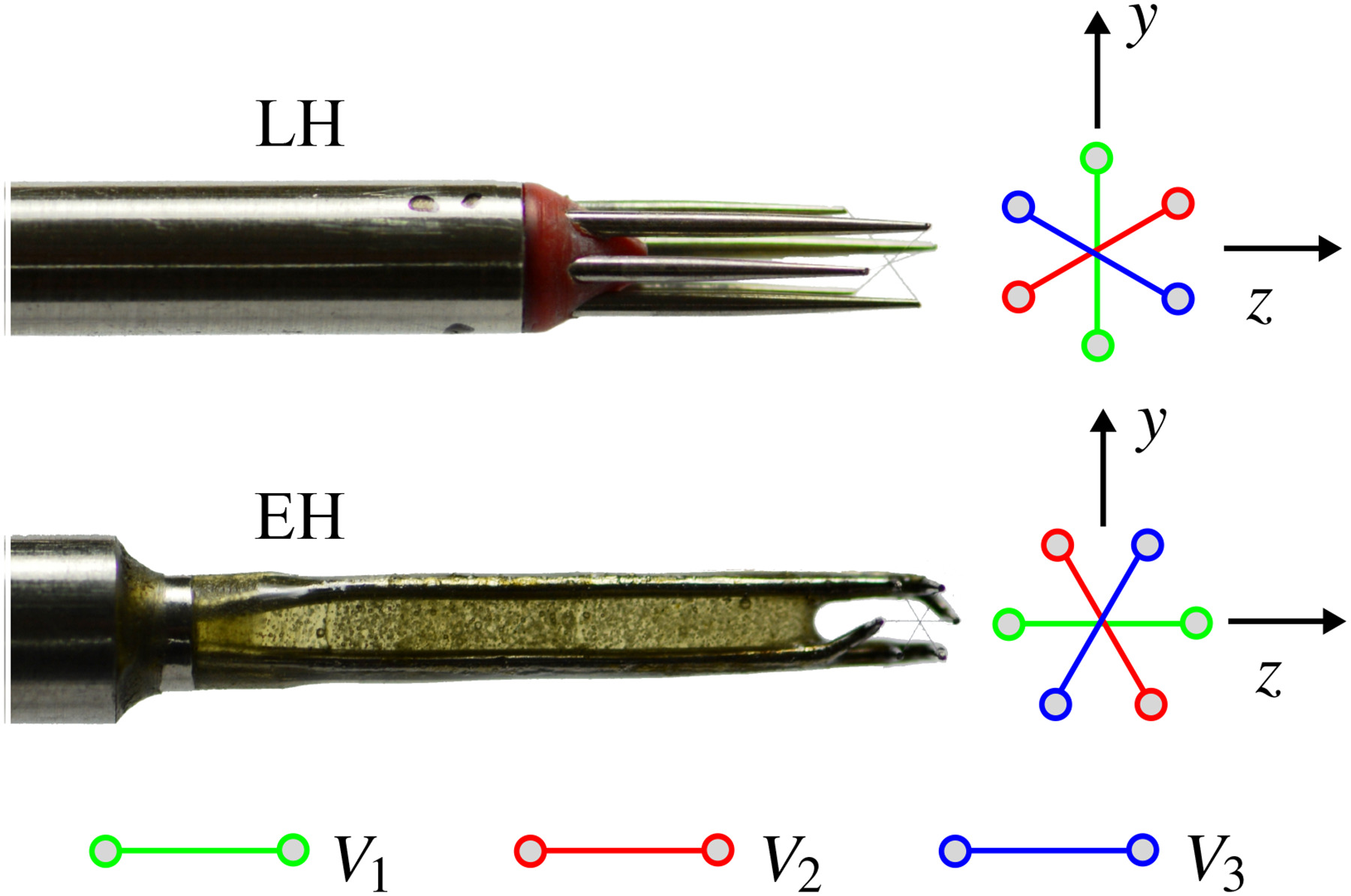
The hot-wire system consists of three Dantec Dynamics StreamLine Pro CTA-bridges and a Spectrum M2i.4721 AD converter board. The experiments used LH and EH probes, both manufactured by Imotec. They are shown in Figure 2 together with the orientation of the wires V1, V2 and V3. Since the LH design requires axial space between blade rows in turbomachines, it is not usually possible to use these probes, even though the impact of the probe shaft on the flow is reduced to a minimum. At the same time, EH probes allow for smaller axial spacing, but the shaft is prone to the flow, and the interaction between shaft and flow can affect the measurements. Both probes were equipped with 9μm platinum-plated tungsten wires. The shaft of the EH probe was oriented in the spanwise (horizontal) direction, and the measurements are denoted by HW EH H. In an additional series of measurements (HW LH 5), the wiring of the LH probe was replaced by a 5μm tungsten wire to evaluate the influence of the wire diameter on the measured data. The length-to-diameter ratio l/d of the wires as well as the corresponding natural frequencies are presented in Table 2. All measurements were carried out with a constant wire temperature of 523K. Due to the constant flow temperature, a constant overheat temperature of the wire can be assumed. The data acquisition was carried out using a sampling frequency of fs=250kHz and a measuring time of t=4s. A square-wave-test, using the procedure of Jørgensen (2002), provides a cut-off frequency for M=0.5 of about 20kHz for the 9μm wire and 65kHz for the 5μm wire.
Figure 2.
Lance-head (LH) and elbow-head (EH) hot-wire probe. The coordinate system refers to the horizontal alignment.
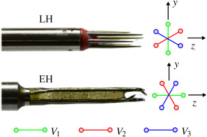
Table 2.
Measured hot-wire l/d-ratios and calculated natural frequencies of the wires.
| Probe | l/d | fn,1 | fn,2 | fn,3 | fn,4 | fn,5 |
|---|
| Lance-head (LH), 9μm | 254 | 7kHz | 19kHz | 38kHz | 63kHz | 94kHz |
| Lance-head (LH), 5μm | 458 | 4kHz | 11kHz | 21kHz | 35kHz | 52kHz |
| Elbow-head (EH), 9μm | 210 | 10kHz | 28kHz | 55kHz | 91kHz | 140kHz |
Data reduction
To derive a relation between voltages measured Vi and flow velocity and flow angles α and γ, the mass flow density (MFD) approach by Poensgen and Gallus (1989) was used. The approach enables HWA measurements in compressible flows. In order to rule out influences due to changing wire properties, the measurements were carried out immediately following the calibration, without any disassembly of the probes. The relation between the calibration and the measurements performed is given by the look-up table approach by Hösgen (2019). The mass flow density MFD=ρc¯ is derived from five-hole probe measurements at identical traverse positions. The five-hole probe measurements provide stagnation pressure and Mach number. Together with the stagnation temperature Tt, the density and velocity are obtained using isentropic relations and the ideal gas assumption. Before the application of calibration to the traverse data, the voltages measured are low-pass filtered (fpass=100kHz) and temperature corrected according to Bearman’s (1971) approach. The velocity components in the coordinate system of the test rig u, v, and w are then derived from the absolute velocity and corresponding flow angles. The mean velocity is calculated according to Equation 2 for an arbitrary velocity ci. N denotes the total number of samples per measurement. By an application of the Reynolds decomposition c=c¯−c′, the velocity fluctuation c′ is obtained. This fluctuation is then used to calculate the Reynolds stresses (Equation 3). The three-dimensional turbulence intensity Tu is defined according to Equation 4.
For studies in the frequency domain, the one-sided auto-spectral density function Gx,c(f) is obtained by splitting the time series into 512 blocks, performing an FFT for each block, and then averaging the single spectra. The cumulative turbulent kinetic energy is defined in Equation 5.
Uncertainty
Measurement uncertainty is calculated on the basis of Hösgen's analytical approach (Hösgen et al., 2016), which uses Gauss’ law of error propagation but distinguishes between systematic and random errors (Grabe, 2011). This approach considers the measuring system itself, such as resolution and noise, as well as uncertainties due to the calibration, pressure correction by the MFD approach, and probe traversing uncertainty. The magnitudes of the uncertainties are given in Table 3. The overall uncertainty is dominated by the fitting error of the calibration, as has been observed by Tresso and Munoz (2000) as well. Given the lack of available correlations, uncertainties due to the frequency response are not considered in the uncertainty assessment. However, one result of the following comparison is that the influence of the turbulent frequency spectrum must be taken into account in the measurement uncertainty analysis.
Table 3.
Uncertainty estimation for the HWA measurements based on Hösgen et al.’s (2016) analytical approach with confidence interval of 95%.
| Freestream | Wake |
|---|
| δ(u¯) (m/s) | δ(v¯) (m/s) | δ(w¯) (m/s) | δ(u′u′¯) (m2/s2) | δ(v′v′¯) (m2/s2) | δ(w′w′¯) (m2/s2) | δ(Tu) (pp) | δ(u′u′¯) (m2/s2) | δ(v′v′¯) (m2/s2) | δ(w′w′¯) (m2/s2) | δ(Tu) (pp) |
|---|
| HW LH 9 | 6.5(5.5) | 2.6 | 3.2 | 0.4(20.2) | 0.1(3.7) | 0.1(1.0) | 0.12(9.4) | 2.0(13.3) | 0.5(11.8) | 0.3(5.2) | 0.23(11.1) |
| HW LH 5 | 5.7(4.7) | 3.0 | 3.8 | 0.3(9.1) | 0.1(2.4) | 0.1(1.0) | 0.10(6.2) | 3.5(13.2) | 1.2(5.2) | 0.3(2.8) | 0.36(8.3) |
| HW EH H | 7.7(6.3) | 2.5 | 5.1 | 0.5(16.4) | 0.2(15.4) | 0.6(7.5) | 0.18(12.8) | 3.8(19.3) | 0.8(24.0) | 2.2(15.8) | 0.48(15.9) |
Laser-doppler anemometry
Hardware
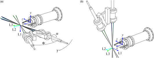
The LDA measurement system used for the present study was a Dantec Dynamics 3D-FiberFlow system with DPSS-Lasers. Two Dantec Dynamics 9061X023 probes with 60mm beam expanders were used for this investigation. One probe measures two orthogonal cartesian velocity components (denoted by L1 and L2) and is aligned on-axis with the test stands coordinate system. The second probe measures an additional velocity component, L3, with an inter-probe angle of Φ≈30∘. With the knowledge of the inter-probe angle Φ, the transformation matrix R can be determined to compute the three cartesian velocity components from the three LDA velocities measured according to Equation 6.
The derivation of the transformation matrix can be found, for example, in Albrecht et al. (2003). Due to the direct measurement of two components, the matrix has several zero-valued coefficients in theory. To eliminate potential uncertainties in the optical setup, an in-situ calibration, which is described in Appendix A, was conducted to determine the transformation matrix R accurately. The in-situ calibration allows for the exact determination of the inter-probe angle Φ and corrects potential errors due to misalignment of the probes with respect to the wind tunnel coordinate system. This ensures the best possible comparability with the HWA measurements.
To enable measurements of negative velocities, a Bragg cell shifts one beam of each channel in its frequency by Δfλ=40MHz. A BSA F80 Burst Analyzer was used to derive the velocity from the back-scattered light. To ensure coincident measurements, the evaluation unit performed a hardware coincidence check that only considered measurements with overlapping Doppler bursts on each channel. Table 4 summarizes the characteristics of the three LDA channels. The significantly smaller spatial extent of the measurement volumes as compared with the hot-wire length (cf. Table 2 with an average length of 2.15mm) is striking. The horizontal setup LD H C (cf. Figure 3a) corresponds to a typical arrangement in turbomachinery testing. Additionally, the probes were rotated around the x-axis to study the effect of the velocity transformation and directly measure the w-component in the vertical setup LD V C (cf. Figure 3b). DEHS seeding was inserted via a Topas aerosol generator ATM242, which provides particle sizes in the range of 0.1μm≤dp≤1μm with a mean diameter of dp=0.25μm. The choice of both the seeding and the seeding device was dictated by the requirement for maximum spectral resolution. Small particles are preferred because the inertia decreases with mass, improving frequency response for higher frequencies (Melling, 1997).
Table 4.
Measurement characteristics of each measurement volume of the three LDA components.
| L1 | L2 | L3 |
|---|
| Wave length λ (nm) | 488.0 | 514.5 | 532.0 |
| Focal length f (mm) | 300 | 300 | 300 |
| Beam pair half angle Θ (∘) | 2.97 | 2.94 | 2.95 |
| Inter-probe angle Φ (∘) | – | – | 30 |
| Measurement volume width dLDA (μm) | 62 | 66 | 68 |
| Measurement volume length lLDA (mm) | 1.20 | 1.27 | 1.31 |
Figure 3.
Setup for LDA measurements with different probe orientations. (a) Horizontal alignment of LDA probe arrangement. (b) Vertical alignment of LDA probe arrangement.
Data reduction
In contrast to the HWA, LDA measurements are triggered by seeding particles that randomly pass the measuring volume. The velocities measured are therefore non-equidistant in time. The measurement data of one particle is composed of the arrival time, the transit time τ through the measurement volume, and a measured Doppler frequency converted into a velocity value. Due to the random character of the measurement, an average data rate is introduced according to N˙i=Ni/t, with N denoting the number of samples for each channel i during the measuring time t. To eliminate the velocity bias (cf. McLaughlin (1973)), transit time weighting is applied. According to Zhang (2010), using the transit time τ as a weighting factor in the computation of the mean velocity (Equation 7) and higher stochastic moments provides an accurate correction. To account for data not necessarily normally distributed, this work uses further correction methods from Benedict and Gould (1996) and the Bessel correction, according to Nobach (2017), to determine the Reynolds stresses (Equation 8).
The derivation of a spectrum from a non-equidistant time signal requires the reconstruction of a uniformly sampled time signal to apply a Fourier-Transformation. This study uses the arrival-time quantization algorithm developed by Damaschke et al. (2018a), which provides a strong estimate of the spectrum up to the average data rate N˙. Unlike simpler algorithms, such as 0th-order interpolation methods, this algorithm does not induce a low-pass filter effect. This effect can be observed in the spectra calculated by the simpler methods above the cut-off frequency of N˙/(2π) and is associated by an f−2-decay in the spectral density (Nobach et al., 1998).
Uncertainty
Corresponding to the HWA procedure, Gauss’ law of error propagation is used to assess the measuring uncertainty. Systematic and random errors are distinguished according to Grabe (2011). Random uncertainties occur as a result of the resolution of the burst detector and noise from the photomultiplier. These uncertainties are of relatively lower importance. Significant sources of uncertainty are caused by the improper alignment of the optical setup, which can lead to fringe distortion as well as velocity bias in flows with an imposed gradient. The uncertainties of both effects are assessed by methods provided by Zhang (2002), Zhang (2010), and Zhang and Eisele (1998). Errors in the Reynolds stresses containing the transformed velocity component are estimated using Albrecht et al.’s (2003) approach, while the uncertainty of the inter-probe angle Φ is assessed using the data from Table 7. Finally, the seeding response to flow fluctuations is assessed on the basis of the Basset-Boussinesq-Oseen equation. Melling (1997) provides Equation 9 to estimate the ratio of the measured variance of a particle movement cp′2¯ to the true variance of the flow c′2¯, as a function of seeding density ρp, its diameter dp, the maximum frequency within the flow fmax and the dynamic viscosity of the flow μ.
Table 7.
Calculated parameter of the transformation Matrix R and mean of the inter-probe angle Φ¯.
| R1,1 | R1,2 | R1,3 | R2,1 | R2,2 | R2,3 | R3,1 | R3,2 | R3,3 | Φ¯ (°) |
|---|
| Rref | 0.000 | 1.000 | 0.000 | −1.000 | 0.000 | 0.000 | 0.000 | 1.732 | −2.000 | 30.000 |
| M0.35 | 0.001 (−) | 0.987 (1.341) | 0.011 (−) | −1.036 (3.580) | −0.011 (−) | 0.010 (−) | 0.017 (−) | 1.687 (2.603) | −1.949 (2.572) | 30.768 (2.560) |
| M0.5 | 0.002 (−) | 0.989 (1.116) | 0.008 (−) | −1.041 (4.051) | −0.009 (−) | 0.008 (−) | 0.017 (−) | 1.764 (1.835) | −2.031 (1.557) | 29.523 (1.591) |
| Mcomb | 0.002 (−) | 0.988 (1.194) | 0.009 (−) | −1.039 (3.889) | −0.010 (−) | 0.009 (−) | 0.017 (−) | 1.735 (0.192) | −2.000 (0.025) | 29.972 (0.093) |
The diameter of the seeding particles is reciprocal to this ratio, and therefore small seeding particles are preferred to resolve flow fluctuations at high frequency. The magnitudes evaluated for the combined uncertainties are given in Table 5. The significant increase of the measurement uncertainty when taking into account the seeding clearly shows the dominant influence of the seeding on the measurement uncertainty.
Table 5.
Uncertainty estimation for the LDA measurements for LDHC.
| Freestream | Wake |
|---|
| δ(u¯) (m/s) | δ(v¯) (m/s) | δ(w¯) (m/s) | δ(u′u′¯) (m2/s2) | δ(v′v′¯) (m2/s2) | δ(w′w′¯) (m2/s2) | δ(Tu) (pp) | δ(u′u′¯) (m2/s2) | δ(v′v′¯) (m2/s2) | δ(w′w′¯) (m2/s2) | δ(Tu) (pp) |
|---|
| w/o seeding uncertainty | 0.2(0.15) | 2.0 | 2.7 | 0.05(0.55) | 0.05(0.60) | 0.06(0.38) | 0.01(0.36) | 3.7(10.66) | 1.46(7.34) | 1.58(5.28) | 0.24(4.63) |
| w seeding uncertainty | 1.7(1.4) | 2.0 | 7.9 | 0.27(3.03) | 0.25(2.88) | 0.28(1.88) | 0.069(2.60) | 4.9(13.15) | 2.0(9.62) | 4.82(12.49) | 0.36(7.71) |
Results and discussion
The following comparison of LDA and HWA is based on the flow at M=0.35. The influence of an increase in the Mach number to M=0.45 is discussed in the final section.
LDA
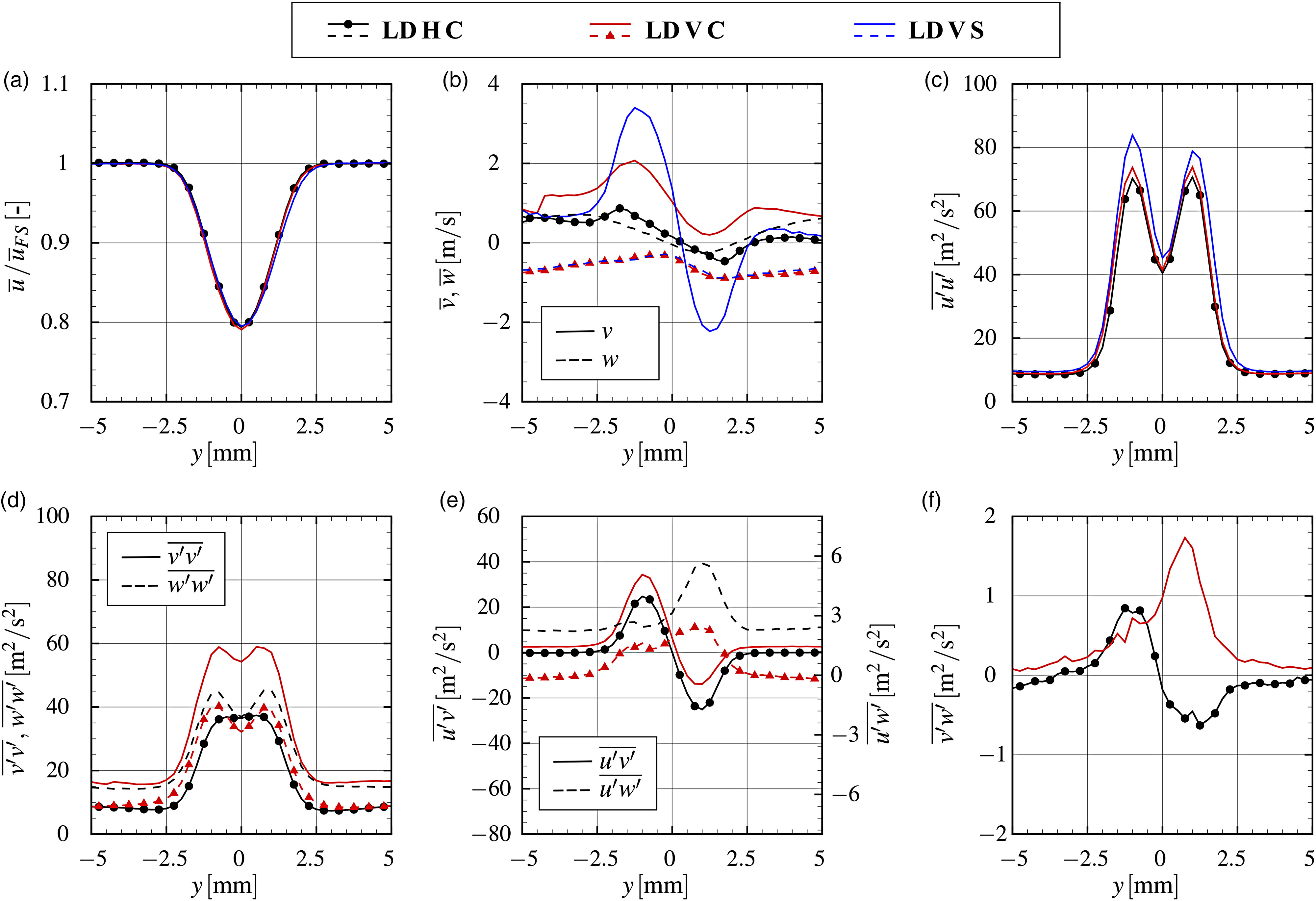
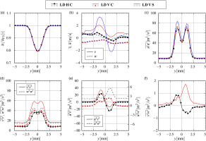
Given its non-intrusive character, the LDA is expected to deliver the most reliable measuring data. However, for the two-probe arrangement, the velocities and Reynolds stresses are usually prone to uncertainties because of the indirect measurement of at least one velocity component. To account for this, this study uses two different probe orientations with regard to the wake generator (cf. Figure 3). This ensures that there are direct measurements of each velocity component in at least one of the two orientations. In the case of the horizontal orientation LD H C, the velocities u and v are directly measured. For the vertical orientation LD V C, these are u and w. The shear stress v′w′¯ is therefore the only quantity that is not measured directly by any of the two setups. Based on these measurements, a reference LDA data set is derived by combining the directly measured quantities from both measurements into a new data set. The reference data set is supposed to have the lowest uncertainty and therefore serves as a basis for comparing the HWA data. The derived mean velocities and Reynolds stresses from both measurements and from the non-coincident measurements LD V S are shown in Figure 4. The data chosen for the reference LDA data set is indicated in the figures by symbols, while lines without symbols are not considered in the reference case.
Figure 4.
Results from horizontal and vertical aligned LDA measurements. Graphs with symbols are used as LDA reference case. The line colors refer to the cases studied, and the solid and dashed lines indicate the different velocity or Reynolds stress components. (a) Streamwise velocity component. (b) Transversal velocity components. (c) Streamwise normal stress. (d) Transversal normal stresses. (e) Shear stresses u′v′¯ and u′w′¯ (f) Shear Stress v′w′¯.
Mean velocities
The measured streamwise velocity component u¯, normalized by the averaged freestream velocity u¯FS at y=±5mm, is shown in Figure 4a. As expected, due to the direct measurement of the streamwise component in each configuration, hardly any differences can be found between the horizontal and vertical alignment. To quantify the difference, the wake velocity deficit uD and the b50-wake width are used. The wake velocity deficit uD is defined as the difference between freestream velocity u¯FS and minimum velocity. The difference in the wake velocity deficit is about ΔuD=0.3m/s between the coincident measurements and 0.5m/s between the coincident and non-coincident vertical alignment measurements. Those differences are of the same order as the measuring uncertainty. No final statement can therefore be made with respect to the impact of the relevant measuring volume in the direction of the gradient. For the LD V C setup, the relevant length is twice as large as for the horizontal setup. The relevant length of the non-coincident measuring volume is 10 times larger compared to LD V C. As such, one would expect a significant change between the coincident and non-coincident measurement, which is not the case here. We therefore expect that the transit time weighting reduces potential deviations as a result of spatial averaging in gradient flows. The b50-wake width (wake width at 50%uD) differs by 0.1mm between all LDA measurements and just 0.04mm between the coincident measurements, which is of the same magnitude as the traversing uncertainty. This indicates a good alignment for both probe orientations and reproducible flow conditions, especially because the trends in velocity deficit and wake widths do not hint at an axial displacement between the probe orientations.
The pitch- and spanwise velocity components v¯ and w¯ are approximately zero, and the measurements differ by a maximum of 1.5m/s between the coincident measurements. This is quite low when compared with the measuring uncertainty, particularly when considering that, for each probe alignment, one of the velocity components is derived from two LDA measurement values. The larger deflections and asymmetry of the v¯-component of the vertical probe alignment may therefore result from the indirect determination based on two measured LDA velocities. Using the transformation matrix R (cf. Equation 6), the ideal transformation formula for the vertical arrangement is given by Equation 10.
It is expected that inaccuracies in each LDA component will be amplified in the calculation of v¯ and that this will result in larger deviations. Since the directly measured velocity components provide lower uncertainty, these measurements are used for the reference data set. The non-coincident measurement shows greater spikes in the case of the indirectly measured v¯-component as compared with the coincident measurement. This is because of the larger relevant measuring volume length and the non-correlated measured velocities cL1 and cL3.
Reynolds stresses
The normal stress in flow direction u′u′¯ (Figure 4c) shows strong agreement between both coincident measurements because of the direct measurement of the velocity component. As expected, the vertically aligned measurements LD V C and LD V S show slightly higher variance within the wake as compared with the horizontal setup LD H C. This is first due to the larger measurement volume and thus an error due to gradient bias. Moreover, incorrect measurements of particles are not filtered out in the case of the non-coincident measurement LD V S, resulting in higher signal noise.
For the normal stresses in span- and pitchwise direction, the measurements already exhibit differences in the freestream region of the flow. The indirectly determined normal stresses are about two times larger than the equivalent directly measured stresses. The reason for this can be found in the (theoretical) transformation formula given for the horizontal aligned setup LD H C by Equation 11.
In addition to the two measured variances cL2′2¯ and cL3′2¯, the covariance cL2′cL3′¯ may have a great impact on the results. For the inter-probe angle of Φ=30∘, this term is even dominant. Both LDA channels see a strong gradient ∂u¯/∂y, while—due to the two-dimensionality of the flow case—there is no significant velocity gradient in the z-direction. Both fluctuations cL2′ and cL3′ therefore tend to be correlated, and the covariance cL2′cL3′¯ is usually positive. In this way, the term containing the covariance in Equation 11 is also positive, and it contributes to a reduction of the normal stress value. As discussed by Albrecht et al. (2003), the covariance is prone to faulty measurements, since the measuring volumes of L2 and L3 intersect at an angle of Φ=30∘. The overlap of both measuring volumes is about ten times smaller than the single measuring volume. In particular, for high seeding density, two particles passing the single measuring volumes outside of the intersection simultaneously can pass the coincidence filter by mistake. As such, a reduced correlation of the cL2′ and cL3′ fluctuations is determined, which relates to an overestimate of the normal stress.
For the shear stresses (Figure 4e and f), a similar trend can be seen as for the normal stresses. The indirectly measured shear stresses u′v′¯ and u′w′¯ in Figure 4e deviate by an offset of 2.5m2/s2 in the freestream from the theoretically expected value of u′v′¯≈u′w′¯≈0m2/s2, which is well met by the direct measurements. After subtracting the offset, the indirect components show strong agreement with the direct measurements. Finally, Figure 4f shows the v′w′¯ shear stress, which is determined indirectly for both measurements. The transformation formula for the horizontal case LD H C is given by Equation (12).
Theoretically, the shear stress should be of zero value for the entire traverse. However, when using the same argumentation as for the covariance cL2′cL3′¯ above, this study is able to explain the graphs well. In brief, it can be stated that the Reynolds stress v′w′¯ will always be faulty when measuring in gradients. However, with a maximum magnitude of v′w′¯=1.7m2/s2, the error can be neglected. Since the graph for the horizontal alignment shows stronger symmetry and lower magnitudes compared with the vertical alignment, it is used for the reference case.
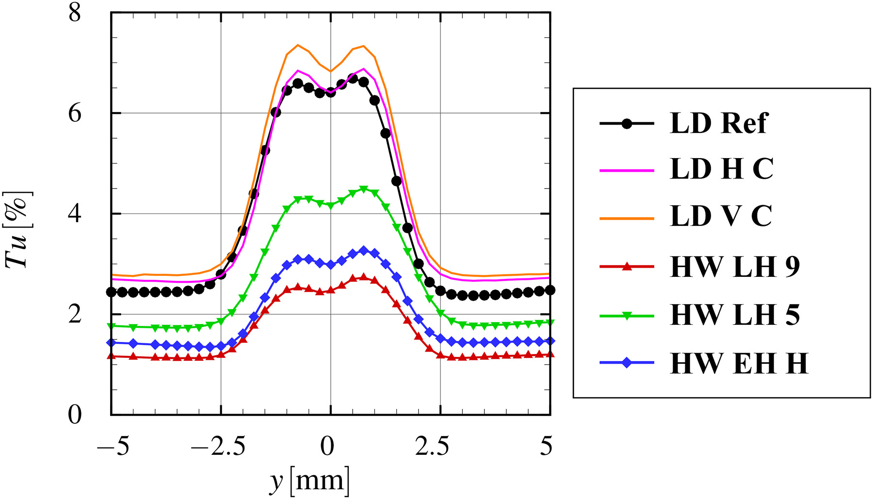
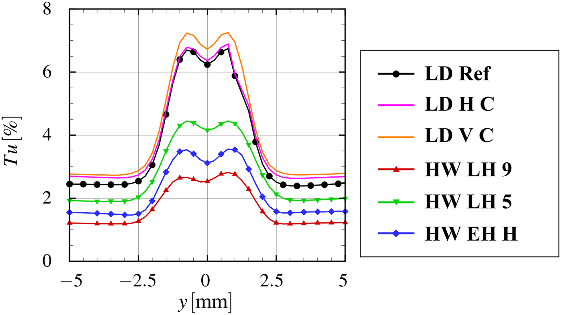
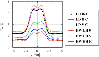
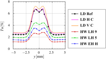
To summarize our findings for the LDA measurements, we note that the measuring technique shows quite strong results for mean velocities, especially when they are directly measured. Moreover, the directly measured Reynolds stresses show strong agreement with the theoretical consideration regarding the expected flow. However, if a velocity or Reynolds stress is derived by a transformation of two or more LDA measurements, deviations and errors are almost impossible to avoid. In most cases, despite the v′w′¯ shear stress, the qualitative course of the measurand is well reproduced. If Figure 5 is taken into consideration, the mistake in the turbulence intensity can be estimated, when using the transformed normal stress, to be of ΔTu=0.22−0.35 percentage points (pp) in the freestream region. This is a relative deviation of 9−14% to the “true” value of the derived reference LDA data set.
Figure 5.
Turbulence intensity measured by HWA and LDA configurations.
Hot-wire
Having derived a reliable LDA data set as reference, different HWA probe designs will be compared.
Mean velocities
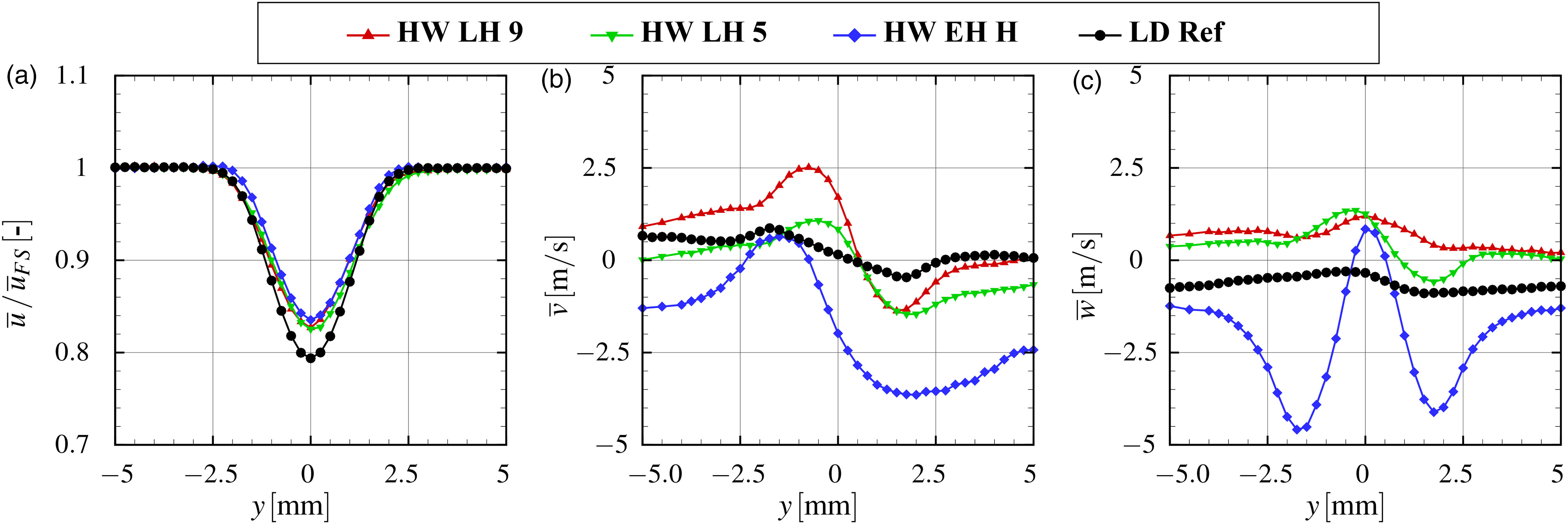
Figure 6 shows the measured mean velocity distributions for the LH probes with 5μm and 9μm wire, the EH probe (9μm wire), and the LDA reference data set. The streamwise velocity u¯ is normalized by the average freestream velocity u¯FS at y=±5mm to eliminate variations due to different test days. However, the absolute value of the components varies by only 1.3m/s between all measurements in the freestream region. Table 6 provides the velocity deficit and wake widths for all measurements. For the displacement and momentum thickness, the incompressible formulations are used according to Equations 13 and 14 to avoid inaccuracies due to the density.
Figure 6.
HWA measurements of averaged velocity components compared to the LDA reference case. (a) Streamwise velocity component. (b) Pitchwise velocity component. (c) Spanwise velocity component.
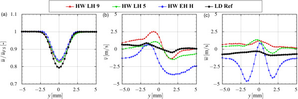
Table 6.
Wake characteristics for M=0.35.
| HW LH 9 | HW LH 5 | HW EH H | LD H C | LD V C | LD V S |
|---|
| uD(m/s) | 20.77 | 20.98 | 19.74 | 24.98 | 25.32 | 24.80 |
| b50(mm) | 2.28 | 2.34 | 2.19 | 2.29 | 2.34 | 2.39 |
| b99(mm) | 4.41 | 4.57 | 3.79 | 4.26 | 4.39 | 4.51 |
| b1(mm) | 0.41 | 0.43 | 0.36 | 0.48 | 0.50 | 0.50 |
| b2(mm) | 0.36 | 0.38 | 0.32 | 0.41 | 0.42 | 0.43 |
The LH probes show similar wake velocity deficits uD, which are about 4m/s lower compared to the LDA reference. The wake width and shape are in good agreement with the LDA measurements, especially for the left side of the wake. On the right side, there is some variation in the transition region between wake and freestream. This is also indicated by the b99-thickness, which is larger for HWA probes as compared with the LDA, while the displacement and momentum thicknesses b1 and b2 are smaller. This is the result of a lower velocity gradient compared to the LDA. The reason for this is the larger measuring volume, which leads to a moving average-like behavior. Applying a moving average to the LDA data shows good agreement in the wake velocity deficit uD between HWA and the averaged LDA data set for an averaging window of 1.5mm. It is reasonable that the averaging window is smaller compared to the probe diameter and wire length because of a varying temperature distribution along the hot-wire. This results in highest sensitivity in the middle of the wire and lowest sensitivity towards the prongs (Bruun, 1995). The EH probe shows a wake velocity deficit which is 1m/s lower compared to the LH probes. Furthermore, the wake thicknesses are remarkably lower compared to the other measurements, while the velocity gradient is similar to those of the LH probes. It is assumed that this is due to an interaction between wake flow and the probe shaft. A similar pattern has been reported by Hölle (2019) for multi-hole pneumatic probes.
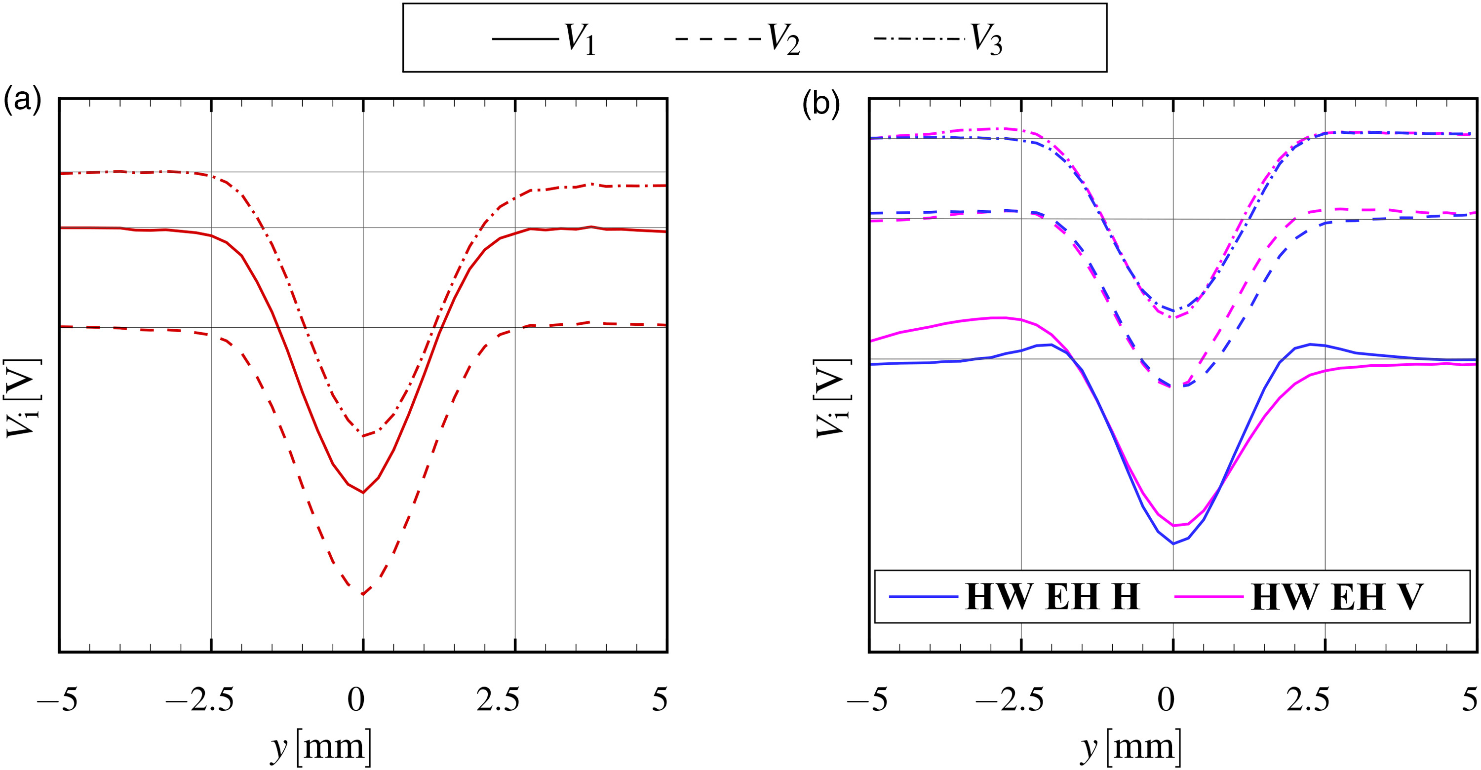
Most striking in the EH probe measurements is a velocity overshoot in the wake to freestream transition, which is the result of an overshoot in the V1-measuring signal (Figure 7b). The overshoot is not visible in the two other wire voltages, as well as in any other signal of the other probes (Figure 7a). At this point the origin of this overshoot is unclear, but it is remarkable that the V1-wire lays in the x−z plane of the test rig, which is not the case for any of the other configurations. The V1-wire is therefore not affected by a velocity gradient along the wire. To check if this is the reason for the overshoot, the vertical alignment HW EH V is used (Figure 7b). The V1-wire is now placed in the x−y plane and prone to the gradient ∂u¯/∂y. As a result, slight overshoots occur in the V2 and V3-signals. The V1-signal now shows strong asymmetries in the freestream region. This indicates a general interaction between flow and EH probe and not an influence of the V1-wire itself. The detailed investigation will be subject to future work.
Figure 7.
Measured wire voltages for the lance-head and elbow-head HWA probes. (a) Lance-head probe (HW LH 9). (b) Elbow-head probe (HW EH H and HW EH V).
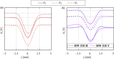
The V1-overshoot also affects the spanwise velocity component w¯, as can be seen in Figure 6c. While the LH probes, as well as LDA measurements show a nearly constant velocity, the graph of the EH probe possesses two minima in the regions of the V1-overshoot and a maximum in the wake mid. The velocity span is 5m/s compared to about 1m/s for the remaining measurements.
The pitchwise velocity component v¯ is shown in Figure 6b. As already discussed in respect of the LDA measurements, this measured component is strongly affected by the measuring volume size. This is because the mean value of each wire is affected by a different velocity gradient and so the slight differences in the measured voltages lead to peaks in the signal. Again, it is shown, that the velocity span is highest for the elbow-head. In contrast to the spanwise velocity component, the overall trend, with a maximum on the left side of the wake and a minimum on the right-hand side, is similar for all measurements of the pitchwise velocity component.
Reynolds stresses
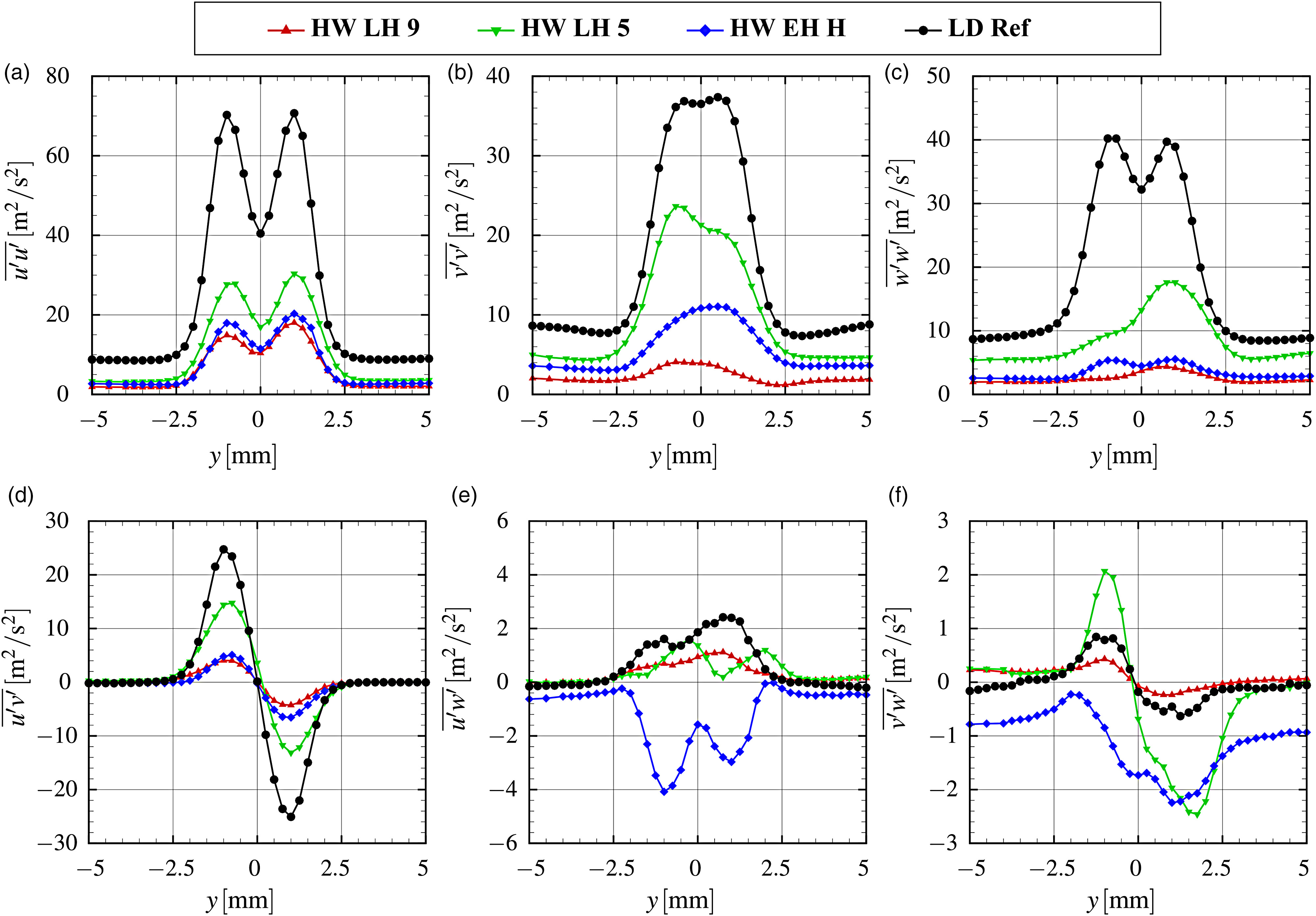
Figure 8 shows the comparison of the measured Reynolds stress tensor. For the normal stresses (Figure 8a–c), the qualitative course is similar between all the measurement configurations. The two peaks in the streamwise normal stress u′u′¯, which result from convecting turbulent kinetic energy from the suction and pressure side of the airfoil, are visible in all measurements. Nevertheless, the magnitude differs between the LDA and HWA measurements by a factor of 4.7 for the LH probe with 9μm wire and a factor of 2.7 for the 5μm wire probe in the freestream region. This difference in magnitude is the result of thermal damping, as the following section on the frequency domain shows. Within the wake region, the absolute difference is even higher, but the scaling remains almost constant. In particular, both 9μm wire probes strongly underestimate the gradients and maxima of the lateral components. The three shear stress components are depicted in Figure 8d–f. For the dominant shear stress u′v′¯, a similar behavior can be observed, but with different magnitudes. Within the freestream region, all measurements show no shear stress, as would be expected on the basis of the theory. The deviation between all measurements is only 0.16m2/s2, which is negligible as compared with the measuring uncertainty.
Figure 8.
Measured HWA Reynolds stresses in comparison with LDA reference case. (a) Streamwise normal stress u′u′¯. (b) Pitchwise normal stress v′v′¯. (c) Spanwise normal stress w′w′¯. (d) Shear stress u′v′¯. (e) Shear stress u′w′¯. (f) Shear Stress v′w′¯.
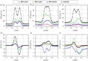
This strong agreement is also not the case for the other shear stresses u′w′¯ and v′w′¯. Indeed, the magnitude is quite small and within the approximated measuring uncertainty. Nevertheless, the EH probe, in particular, shows a different behavior from the other measurements. The freestream value of pitchwise and spanwise shear stress differs from zero, which does not fit to the theoretically expected behavior. For the u′w′¯ stress, the EH probe reveals only negative values across the wake, while all other measurements show positive values. The way in which measurements in three-dimensional flows are affected by this should be the subject of a future investigation.
To conclude the findings for the integral values, Figure 5 shows the three-dimensional turbulence intensities across the wake. As previously mentioned, the LDA measurements differ in the freestream region by about ΔTu=0.2pp compared to the reference data set. The HWA measurements deviate by ΔTu=1.3pp for the 9μm LH probe and ΔTu=0.7pp for the 5μm LH probe. The EH probe shows a freestream-turbulence intensity slightly higher than the 9μm LH probe. Within the wake, HWA and LDA measurements differ by up to ΔTu=4pp for the 9μm wire and ΔTu=2.3pp for the 5μm wire.
Frequency domain
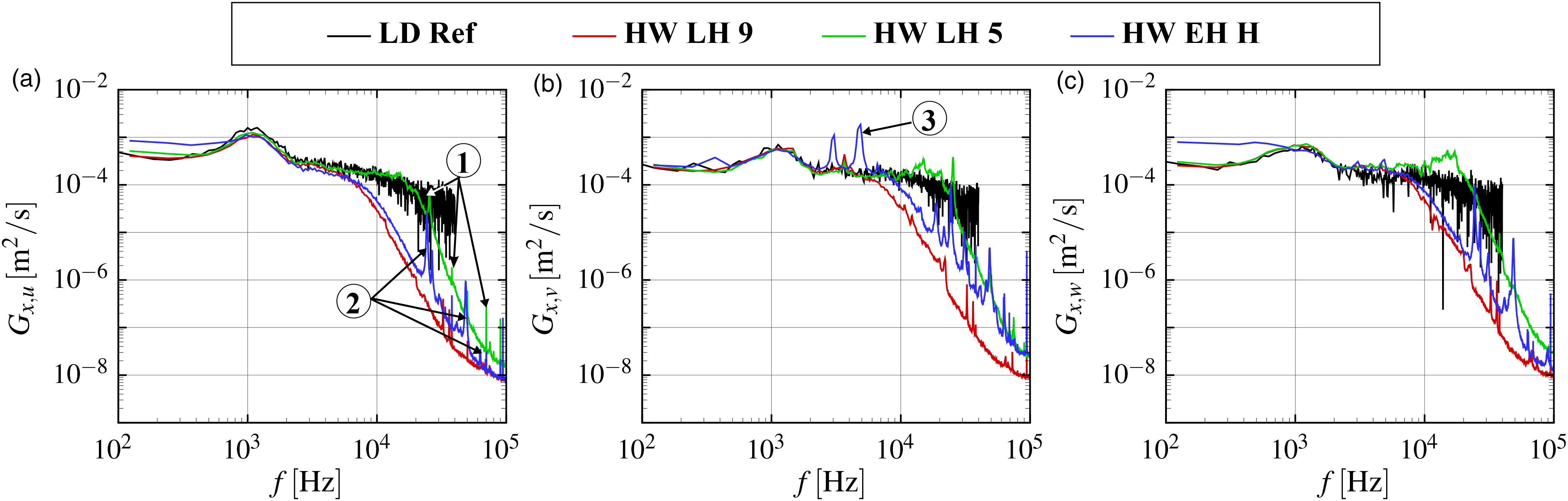
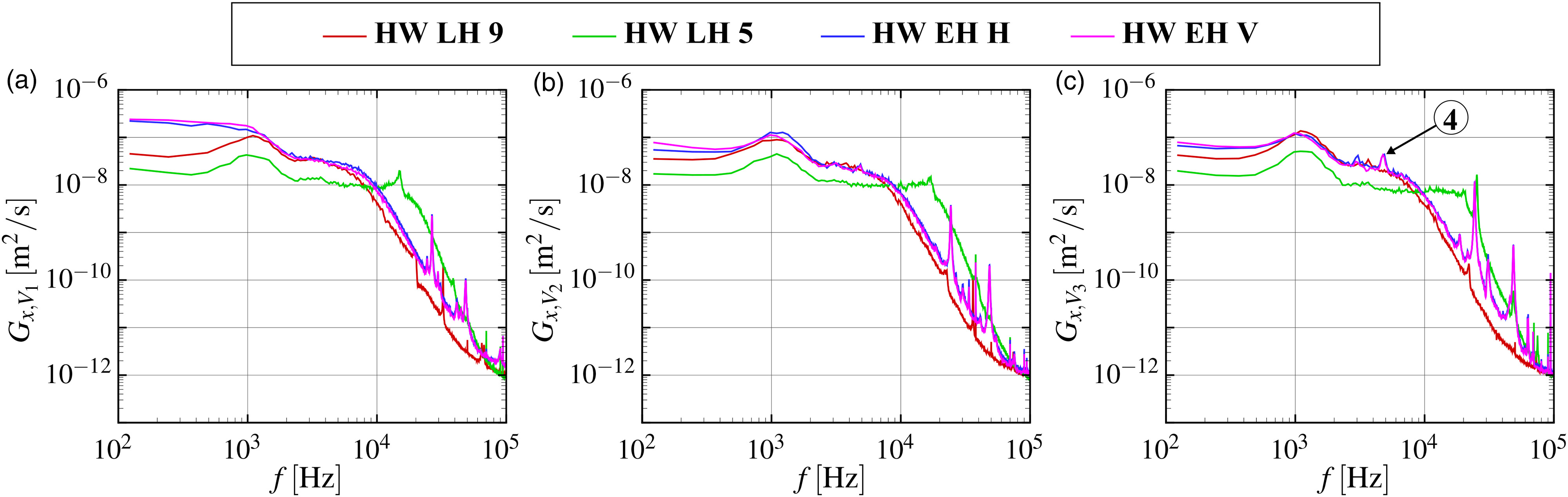
The auto-spectral density function of the HWA and LDA measurements are shown in Figure 9 for the freestream position y=5mm. As the coincident 3D LDA data set is lacking in accuracy in the third component, the velocity components are considered separately to ensure a fair comparison. First, the low frequency domain up to f=2.5kHz is considered. In this region, the LDA data and the LH probes show nearly identical spectra for all velocity components (Figure 9a–c). Even the test rig-specific peak at f=1kHz is reproduced accurately. For the EH probe the amplitudes of low frequency u′- and w′-fluctuations are on an elevated level as compared with the other spectra. As seen in Figure 10a, the cause for this is the V1-voltage signal measured. To clarify, if it is a flow-related feature, the vertical probe arrangement HW EH V is considered. Since the signals V1, V2 and V3 do not change due to the rotation of the probe, it can be stated that the relatively higher energy amount in the low frequency region results from the probe head design and is specific to the V1 component. This phenomenon has also been observed for other EH probes with identical prong arrangements, which confirms the head design dependency. Moreover, the strong agreement between the horizontal and vertical EH probe in Figure 10 shows that the turbulence at the freestream position would appear to be almost isotropic, as there are barely any changes in all voltage signals.
Figure 9.
Power-Spectral-Density of u, v and w for the freestream-position y=5mm. (a) PSD(u). (b) PSD(v). (c) PSD(w).
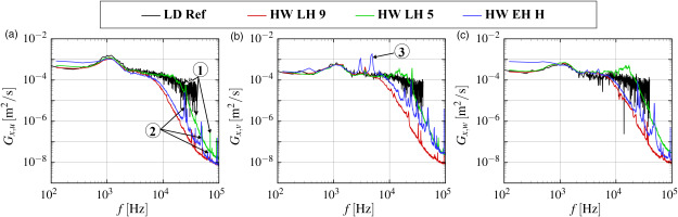
Figure 10.
Power-Spectral-Density of measured HWA voltages for the freestream-position y=5mm. (a) PSD(V1). (b) PSD(V2). (c) PSD(V3).

Larger deviations between the investigated probes can be seen in the high-frequency region, starting at f=2.5kHz. Four topics will be addressed in the following section: 1. the impact of the HWA diameter; 2. the vibration of the HWA wires; 3. the frequency excitation of the EH probe, and 4. the effect of seeding.
The impact of the HWA diameter
General application rules for hot-wires state that the hot-wire length l should be similar to the smallest scale in the flow, namely the Kolmogorov scale (Tropea et al., 2007). At the same time, the wire length should be large enough to prevent heat conduction into the prongs. Ligrani and Bradshaw (1987a) therefore recommend a length-to-diameter ratio of l/d=200 for a platinum wired probe. Nevertheless, these guidelines are hard to fulfill for turbomachinery flows where the integral length scale may already have a dimension of 0.2mm. To develop an initial impression for the magnitude of the wire geometry's impact, we replaced the 9μm wire by a more fragile 5μm wire and in this manner raised the l/d ratio. When the LH probe measurements in Figures 9 and 10 are compared, all spectra show strong agreement between both wire diameters up to f≈5.6kHz. For higher frequencies, the 9μm wire probe spectra drop sharply by about f−4.7. The amplitudes of the 5μm wire spectra remain almost constant up to f=15kHz and then drop by f−7. In both cases the drop is far above the f−5/3 decay of the theoretical Kolmogorov spectra and starts below the frequency limit obtained by the square-wave test. It is therefore expected that the different damping is the result of higher heat conduction in the prongs in case of the thicker wire, which leads to lower sensitivity. The EH probe shows a slightly higher cut-off frequency as compared with the 9μm LH probe even though the l/d-ratio is smaller. This can be explained by the determination of the decade resistance of the CTA bridge. The resistance of the wire is determined by measuring the total resistance of the wire, prongs and support leads. The prong and support lead resistance is then determined by replacing the probe with a shortening device. Since the resistance can differ slightly between probe prongs and shortening device, this can lead to a different effective overheat temperature (Ligrani and Bradshaw, 1987b). For the LH probes, this effect was excluded by using identical probes.
The vibration of the HWA wires
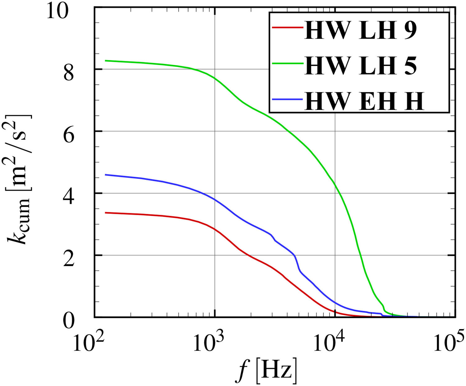
All of the HWA measurements in Figure 9 show peaks at discrete frequencies that vary slightly by wire and diameter. Table 2 provides the natural frequencies of the first five modes of the wires for each probe, which were calculated by assuming a double-clamped beam. For the LH probe with 5μm wire and the EH probe, the second, third, and fourth natural frequency modes can be clearly identified. These frequencies are marked by ① and ② in Figure 9a. Hösgen (2019) has shown that these wire vibrations might have a significant impact on the measured turbulence intensity and turbulent kinetic energy. However, for the current flow, we do not identify any significant jumps in the cumulative turbulent kinetic energy kcum at relevant frequencies (cf. Figure 11), and we therefore did not apply any filtering.
Figure 11.
Cumulative turbulent kinetic energy for the HWA measurements in the freestream (y=5mm).
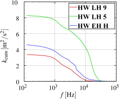
The frequency excitation of the EH probe
In addition to the previously mentioned frequency peaks, there are also frequency peaks in the HWA spectra that seem to be probe-dependent, such as the peaks ③ and ④ in the EH probe spectra around f=4.8kHz in Figures 9b and 10c. As can be seen in Figure 11, the cumulative turbulent kinetic energy kcum is raised by this oscillation. Since this frequency is only observable in the V3 signal, it has to be a probe-related issue. Using the Strouhal number of Sr=0.21 to assess potential flow-related vibration excitations of the probe, reasonable indications of an excitation of the outer prong of the V3 wire were detected. By filtering this frequency, the turbulent kinetic energy is reduced by Δk=0.3m2/s2, which is equal to a relative change of 7% as compared with the unfiltered data.
The effect of seeding
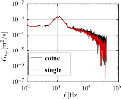
Finally, the LDA spectra are considered. The increased noise with increasing frequency is a typical result of advanced spectra reconstruction algorithms, as shown by Damaschke et al. (2018b). Up to f≈10kHz, the LDA spectra show strong agreement with the 5μm wire LH probe. For higher frequencies, the spectra drop by approximately f−2. For the coincident measuring mode, the average data rate for this measuring point is N˙=14.2kHz, which is equal to the limit of the algorithm's prediction. To check whether the decay is a damping effect due to the limited data rate, we conducted additional non-coincident LDA measurements with higher average data rates of approximately 42kHz. The spectra of the streamwise velocity components are shown in Figure 12. As the data rate for the non-coincident measurement is three times higher than for the coincident measurement, a significant deviation should be visible. However, this is not the case, and therefore we assume that the decay is due to the seeding response to flow fluctuations. In the worst case for a particle diameter of 1μm diameter, the relative fluctuation intensity, according to Equation 9, is only cp′2¯/c′2¯=86%. The greater the frequency, the lower the particle response even for smaller particles. The assumption therefore is that the decay is the result of the damping of different particle sizes.
Figure 12.
LDA spectra from coincident and non-coincident (single channel) measurements.
Impact of Mach number
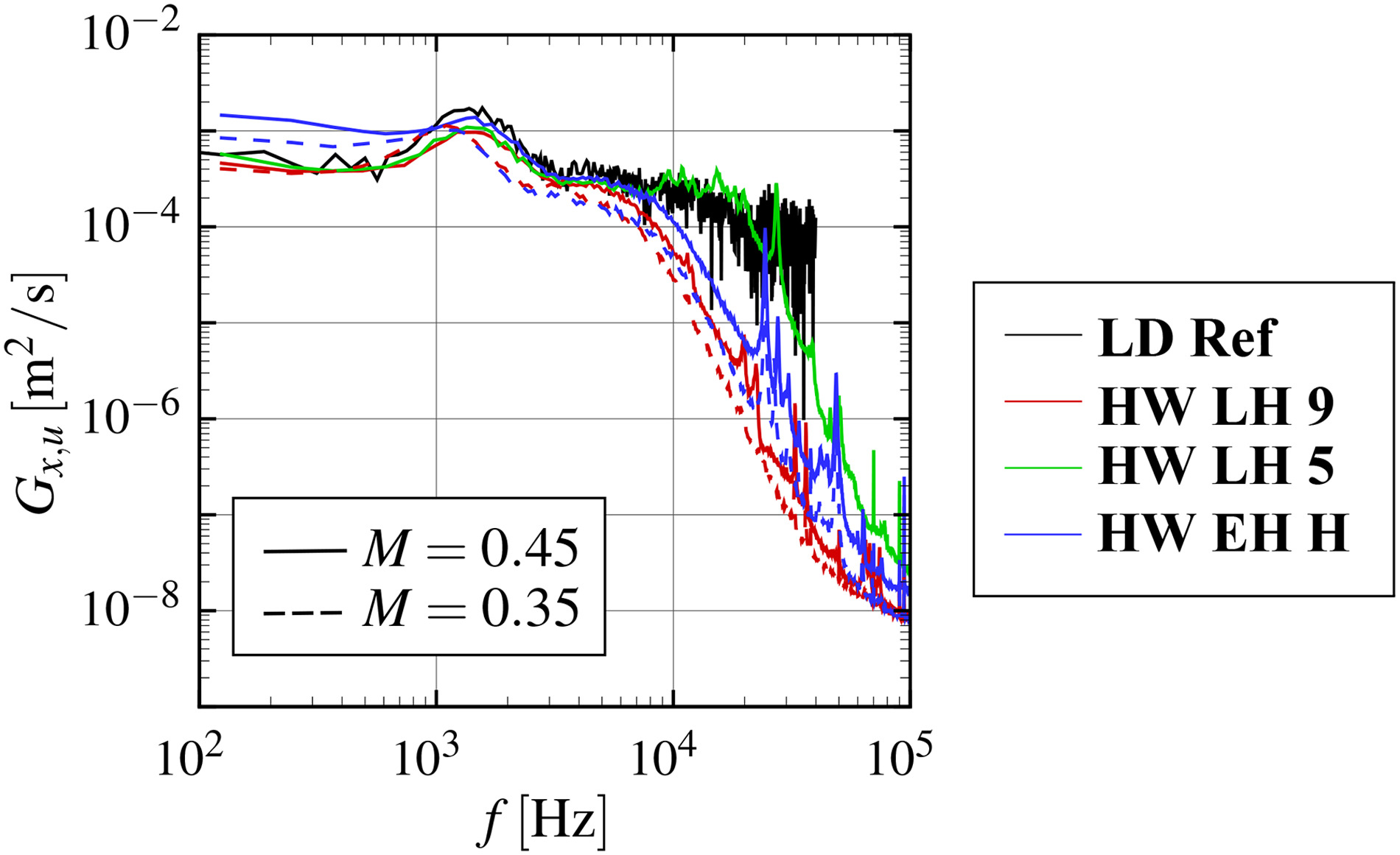
As a final part of the investigation, the Mach number was raised to M=0.45. The main results are shown in Figures 13 and 14. The most important outcome of the spectra for the streamwise velocity component (Figure 13) is that the damping frequencies of the hot-wires are shifted towards higher frequencies by approximately 1kHz for the 9μm wires and 2.5kHz for the 5μm wires. Moreover, the LDA damping frequency does not change. The Mach number variation is also helpful in distinguishing between flow-related frequency excitation and probe-related natural frequencies. The natural frequencies change with neither the Mach number nor the velocity, as can be seen from the wire frequencies. Flow-related characteristic frequencies increase with an increasing Mach number or velocity. In general, when increasing the Mach number, further problematic frequency ranges have to be considered for HWA measurements. This means that spectra in the high frequency regime become noisier and making a distinction between wanted and unwanted frequencies gets more difficult. Figure 14 shows the turbulence intensities for M=0.45. There are no significant changes as compared with the lower Mach number of M=0.35 (Figure 5). The relative deviation between the LDA reference and LH probes is reduced by approximately 2% for the 9μm probe and 6% for the 5μm probe, which is due mainly to the increasing damping frequencies.
Figure 13.
Comparison of auto-spectral density of the streamwise velocity at M=0.45.
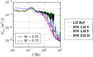
Figure 14.
Turbulence intensity measured by LDA and HWA at M=0.45.
Conclusions
In this study, an LDA reference case has been established to compare 3D-LDA and 3D-HWA measurements with respect to probes used in turbomachinery. While the average velocity components show the expected behavior, such as a reduced wake velocity deficit due to differences in the measuring volume size, this study has found major discrepancies in the measured Reynolds stresses. The main findings are as follows:
If only one optical window is used for LDA measurements, the measurement of the third component always contains errors. For the present flow, the turbulence intensity is overestimated by 13% in the freestream compared to an alignment, where all velocity components are directly measured (e.g., 2-window-arrangement).
The main discrepancy between LDA and HWA measurements is the result of damping effects in the HWA measurements. Reducing the wire-diameter from 9μm to 5μm leads to a 35% increase in the measured turbulence intensity.
The invasive character of the HWA leads to an excitation of certain frequencies, which leads to a higher turbulence intensity measured. The discrepancy to LDA measurements regarding the turbulence intensity is reduced, but the effect is not flow-related and should be filtered.
EH probes, which are commonly used for measurements in the axial gap between blade rows, are even more prone to detrimental effects, such as vibrations, than LH probes. In this study, the different probe head used leads to an overestimation of the turbulence intensity by 23% compared to the LH probe.
Increasing the Mach and Reynolds numbers leads to slightly higher damping frequencies for the HWA, and the discrepancy in turbulence intensity between LDA and HWA is therefore reduced.
The observed total relative deviation in turbulence intensity between HWA and LDA measurements is about
50% for the
9μm wire and
27% for the
5μm wire in the freestream region. The discrepancy increases in the wake region due to the increasing amount of high frequency fluctuations that are not detected by the HWA. Even though the application of HWA probes revealed many drawbacks, a strong qualitative agreement between the measured traverses was obtained for the key Reynolds stresses. The HWA scores in terms of robustness, simplicity of application, and speed of measurements. For the present study, it should be stressed that no conclusive verdict statement can be made as to which of the two measurement techniques is more accurate. After all, this is more a comparative study that reveals the drawbacks of each measuring technique. In our future research, we plan to more deeply examine how the EH probe affects the hot-wire measurements and derive corrections for both HWA and LDA measurements. Therefore, we plan to set up additional well-defined flow test cases with known spectra.