Experimental setup

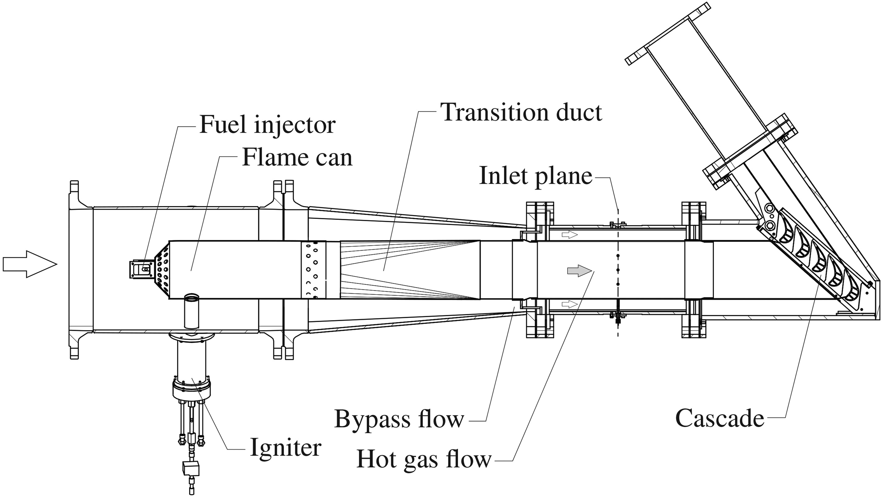
The Linear High-Temperature Cascade (LHTC) at the Institute of Jet Propulsion and Turbomachinery is a test rig designed to test cooled turbine blades at high temperatures and realistic density ratios (Findeisen et al., 2017). Currently, the rig is being used to test and validate film-cooled turbine blades as part of a research project. The rig can operate at main flow temperatures of up to 1,300K and hot gas mass flows of up to 1.2kg/s, generated by an engine combustion chamber. Figure 1 shows the cross section of the LHTC, which comprises five turbine blades. The main stream air flow is supplied by a compressor with up to 5kg/s. A diesel-fueled combustion chamber heats the main flow to up to 1,300K. The test rig has two flow paths downstream of the flame tube. The bypass flow serves as a cooling system for the inner hot gas ducts and ensures thermal decoupling of the outer housing. Three traversable, water-cooled total temperature and total pressure probes are located in the straight section downstream of the transition duct. These are used to measure a two-dimensional flow inlet profile. Three static pressure taps are installed upstream of the probes. These measurements allow the operating point to be characterized. Due to the high temperatures and locally varying concentrations of exhaust gas, the transport and material properties of the flow differ noticeably from those of dry air. Hence, they are calculated for every measurement point using Cantera (Goodwin et al., 2023) and a diesel surrogate fuel model (Pei et al., 2015). On this basis, the mass flow m˙HG of the hot gas flow and a mass flow averaged operating point can be calculated. The flow is characterized by the Reynolds number in the hot gas flow

Figure 1.

Section View of the Linear High-Temperature Cascade.

where L is the chord length, A the cross section area of the inlet section and μ the dynamic viscosity. The latter is also calculated with Cantera on the basis of the calculated flow conditions. All the results presented were obtained at ReHG≈120×103.

Blade configuration and instrumentation

The cascade is comprised of five blades, of which the outer blades form the wall for the hot air flow, while the three blades in the middle of the cascade are used for temperature (middle blade) and pressure measurements (adjacent blades), cf. Figure 2. The blade cooling design is derived from the mid-section of a high-pressure turbine blade and features four smooth internal cooling channels. The three middle blades each have 18 cylindrical film cooling holes which are located on the suction side of the first channel. To ensure mass conservation in the fourth channel, trailing edge ejection is not utilized. The blades are mounted in the test rig with the tip plates facing downwards. The middle blade is equipped with a total of 66 thermocouples to measure the metal temperature of the blade. Of these, 32 thermocouples are located in the mid-plane, while 16 thermocouples are located in both the hub and tip planes at 10% and 90% of the blade height respectively.

Figure 2.

Test blades with measurement locations. (a) Mid-section of the tested blade showing the cooling channels and the location of the film cooling row with 18 cylindrical film cooling holes at s/L≈0.35. (b) Top view, (c) Side view of the three middle blades. The middle blade is equipped with thermocouples, while the adjacent blades have holes for profile pressure measurements.

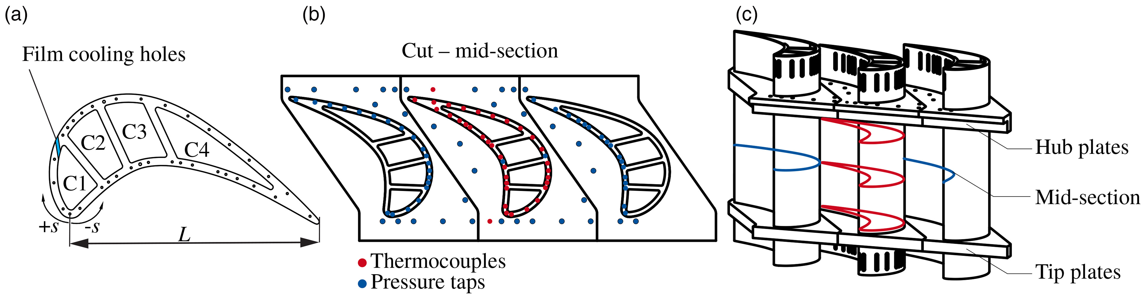
The blades to the left and right of the center are used for measuring the profile pressure at a total of 37 pressure taps. Based on the profile pressure the isentropic Mach number

(2)

Mais=2κ−1[(pt,HGp)((κ−1)/κ)−1]

is calculated, where p_t,_HG is the main flow total pressure at the inlet plane and κ the isentropic exponent of the main flow exhaust gas. Additionally, 34 pressure taps are located at the tip plate (cf. Figure 2) to measure the static pressure at the cascade inlet and outlet as well as in the passage between the blades.

Blade cooling

The cooling air is provided by a separate compressor and can be heated by a flow heater to up to 573 K. A total of six valves are used to control the mass flow to the blades. Figure 3 shows the cooling air supply and tubing for the central blade. Air is supplied to the entrance of channels 1 and 2 from the flow heater. Instead of using the usual internal deflection, the cooling air is guided out of the blade and deflected to a pipe section before entering the next cooling channel. After passing channel 1, the cooling air is blown out into the bypass flow. The cooling air from channel 2 is guided through pipes outside the blade and redirected into the following channels 3 and 4. Downstream of channel 4, the cooling air is blown out into the bypass.

Figure 3.

External cooling air pipes of the central measurement blade, (a) top side and (b) bottom side of the blade. Static pressure, total pressure and temperature are measured at each channel inlet and outlet.

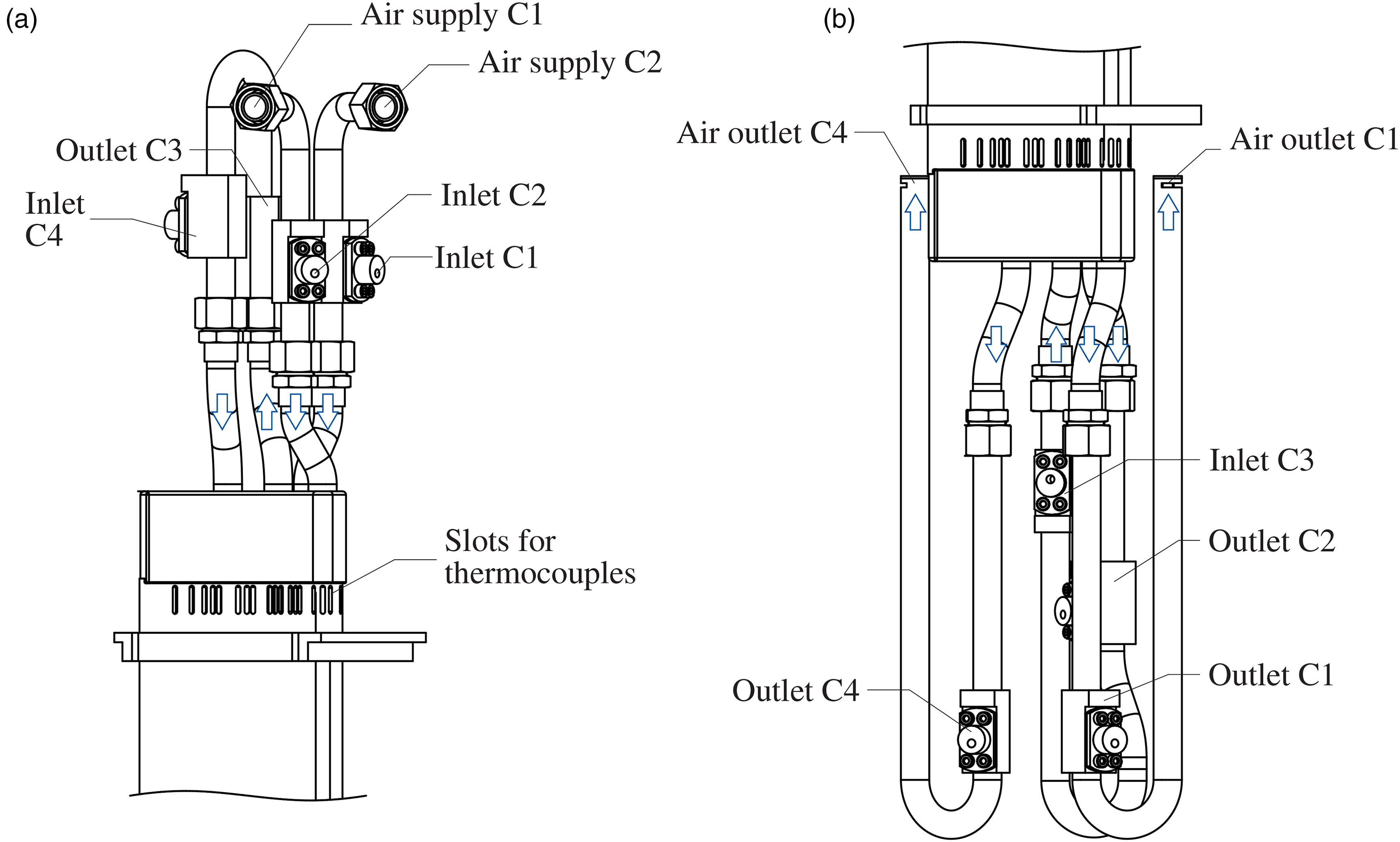
To characterize the cooling air flow, cooling air measurement sections (CAM) are used. Six CAMs are placed at the cooling air inlets of the three middle blades, so that each inlet is measured separately. Six more CAMs are placed in the external cooling air path of the middle blade (cf. Figure 3), so that there is one measurement section upstream and downstream of each channel respectively. This enables the measurement of inlet and outlet quantities at each of the four cooling air channels of the center blade. These values serve as boundary conditions for CFD calculations of the blade.

Each CAM contains a combined Kiel head probe for total pressure and total temperature measurements (cf. Findeisen et al., 2017). Additionally, three pneumatically averaged static pressure taps are located upstream of the Kiel probe to determine the Mach number, which is used for recovery factor correction of the total temperature probe. The coolant mass flow m˙C can be calculated on the basis of values for total pressure, temperature and static pressure. Due to the existence of boundary layers and inhomogeneous velocity profiles, every CAM is calibrated in-situ with an EN ISO 5167-2 compliant measurement orifice. With this calibration the uncertainty of the CAM mass flow is approximately 0.9×10−3kg/s, which depends slightly on the coolant temperature and total pressure.

The operating point of the cooling air is determined by the combination of coolant temperature TC and the coolant mass flow m˙C. We use the ratio of the density of the coolant fluid to that of the main flow DR=ρC/ρHG as a similarity parameter. For the first channel, where the film cooling holes are located, the ratio of film cooling to main stream mass flow is used

(3)

MR=m˙Cm˙HG=m˙C1,in−m˙C1,outm˙HG.

The film cooling mass flow m˙C is the difference between the inlet m˙C1,in and outlet mass flow m˙C1,out of channel 1. When MR is changed, the mass flow in channel 2 is set equal to the mass flow of channel 1 m˙C1,in=m˙C2,in. To characterize the convective cooling the total coolant to main stream ratio

(4)

TCR=m˙C,totm˙HG

is used, where m˙C,tot is the sum of the inlet mass flow of channel 1 and 2.

Numerical setup

Steady-state conjugate heat transfer (CHT) simulations were performed to analyze both the aerodynamic characteristics and the thermal conditions of the blades. The numerical setup shown in Figure 4 is composed of the hot gas domain, the cooling air domain and the solid blade domain. Separate computational meshes were created for each domain using Ansys ICEM CFD. Ansys CFX was used for all steady-state simulations. The hot gas domain featured only one passage of the test rig with periodic boundaries in pitchwise direction. At the inlet, total temperature and total pressure profiles from the inlet probes were used. Since there is no pressure measurement downstream of the cascade, the outlet static pressure was adjusted to match the blade surface pressure distribution of the experimental data. The hot gas was modeled as an exhaust gas consisting of N2, O2, CO2 and H2O with temperature-dependent fluid properties. For the cooling air domain, the cooling air pipes were split at each CAM. In this way, the inlet (total temperature and total pressure) and outlet (static pressure) boundary conditions can be directly adopted from the respective experimental CAM data. The cooling air was modeled as dry air consisting of N2 and O2 with temperature-dependent fluid properties. The first cooling channel featured a fluid-fluid interface with respect to the hot gas flow, allowing the cooling air to pass through the film cooling holes into the main stream.

Figure 4.

Computational domain and mesh used for CFD simulations.

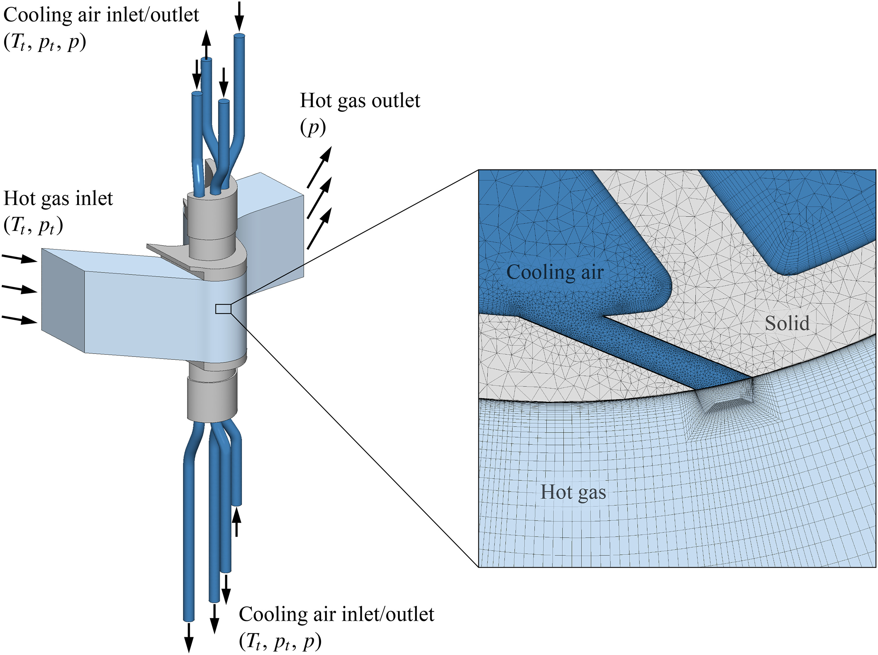
The solid domain is placed between the hot gas and the cooling air. The thermal conductivity of the solid matches the properties of Alloy X. Fluid-solid interfaces are defined on the walls adjacent to the hot gas or cooling air flow respectively. All walls located within the bypass are almost adiabatic due to the thermal insulation in the test rig.

All simulations were carried out using both the k-ω-SST turbulence model (Menter, 1994) and the BSL EARSM (Wallin and Johansson, 2000), each in combination with the γ-Reθ transition model (Menter et al., 2006). Since the results of the BSL EARSM model were in better agreement with the experimental data, only these results are presented here. Three different levels of mesh refinement were investigated and differences in the film cooling region were observed across all mesh levels. A finer mesh was not considered due to excessive computational cost. Consequently, the finest mesh was selected for the simulations. This mesh contains a 60 million elements structured mesh for the hot gas domain to accurately resolve the film cooling flow entering the hot gas flow and a 40 million elements unstructured mesh for the cooling air channels. As a result, an average non-dimensional wall distance of y+=0.3 was achieved in the fluid parts. Additionally, an unstructured grid of 10 million elements was created for the solid blade.

Based on the simulation results, the momentum ratio I of the film cooling flow can be calculated

The momentum of the main flow (ρc2)HG is calculated using the pressure and the isentropic Mach number (Equation 2) at the film cooling row. It is important to note that the momentum ratio cannot be measured in the experiment.

Inlet conditions

The inlet profile of the main flow for the following results is shown in Figure 5. The temperature profile at the inlet shows a significant gradient in the vertical direction (z), with temperature peaks located above the channel mid-plane. A thermal boundary layer is visible near the hub. The total pressure near the tip is significantly lower than at the hub, which can be explained by the interaction between the rotation-symmetric temperature profile generated by the fuel nozzle of the flame can and the liner. The transition duct changes the circular cross-section of the combustor the rectangular shape of the inlet section. This transition involves a reduction in channel height to half the diameter of the combustor section, while maintaining a consistent channel width, which results in the following two effects. First, the rotation-symmetric temperature profile contracts vertically. Second, the resulting non-uniform flow acceleration induces a secondary flow that transports cold fluid from the near wall towards the hot gas mid-plane (Mick et al., 2013). These overlapping effects explain the observed total temperature and pressure profile, which remains consistent for all operating points.

Figure 5.

Normalized total pressure and temperature profile at the inlet section for ReHG=120×103. Each cross is a measurement point, values in between are linear interpolations.

Validation of the CFD results

CFD simulations were used to get a more detailed view of the flow field and the heat transfer of the blade. A comparison between the experimental data and the numerical results is shown in Figure 6. The left-hand diagram illustrates the isentropic Mach number Mais in the mid-plane of the blades. In the right-hand diagram the normalized blade material temperature is shown for two different mass flow ratios. Overall, the numerical results are in good agreement with the measured material temperatures. However, downstream the film cooling row the CFD simulations overestimate the material temperatures on the suction side from s/L>0.8.

Figure 6.

Comparison between the experimental data and the CFD simulations for OP2. Left: isentropic Mach number. Right: blade material temperature.

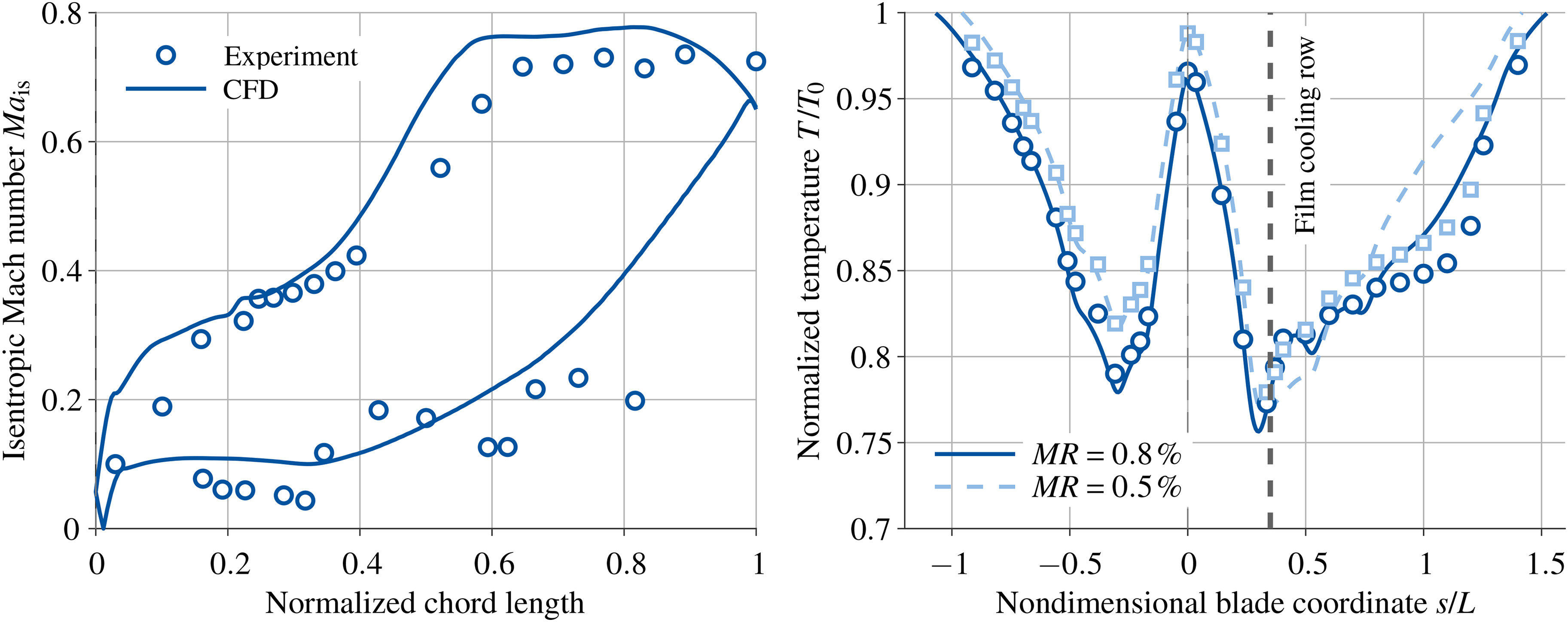
Experimental results

Effect of varying coolant mass flow ratio

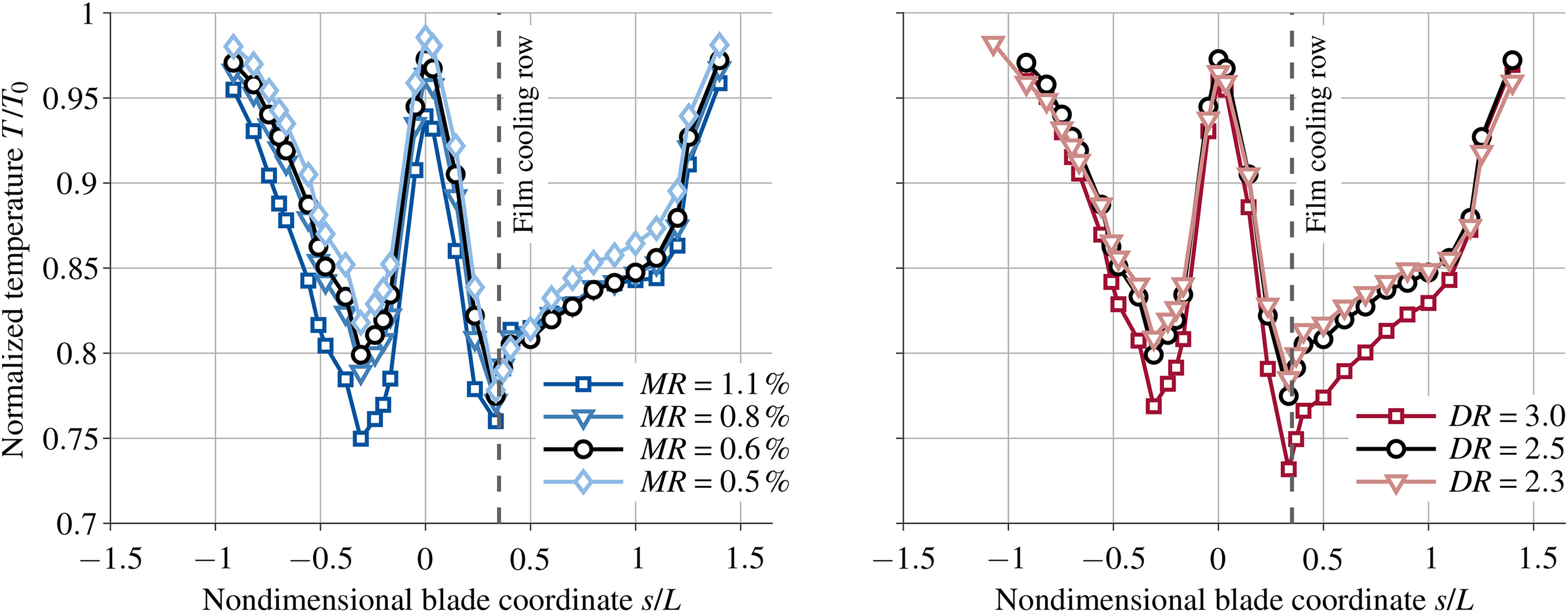
Figure 7 shows on the left-hand side the normalized blade temperature of the film-cooled blade for four different mass flow ratios. As the coolant mass flow increases, the material temperature generally decreases due to the higher overall cooling air flow. This effect is particularly noticeable on the pressure side which is only convectively cooled and on the suction side upstream of the film cooling row. The design of the blade causes film cooling and convective cooling to interact. A high film cooling mass flow requires high pressure in the cooling channels due to the significant pressure loss at the exit of the film cooling holes. However, the pressure resistance for the internal cooling flow, which determines the mass flow, remains almost constant. The total mass flow therefore increases disproportionately when MR is increased. For instance, an MR of 1.1% leads to a TCR that is twice as high as for MR=0.8%. However, when MR is low, TCR also decreases, resulting in a lower absolute heat flow in channel 2-4 and an increase in material temperature.

Figure 7.

Normalized material temperature at the mid-section plan for different coolant mass ratios MR left and for different coolant density ratios DR right. The black colored graph shows the same operating point in both diagrams.

Downstream of the film cooling holes s/L>0.35, an increase in film cooling mass flow does not result in a reduction in the material temperature. Only at very low mass flow ratios of 0.5%, does the blade temperature increase due to the reduced total mass flow. Directly behind the film cooling holes s/L≈0.4, the temperature actually increases as the cooling mass flow increases. This is most likely due to the separation of the cooling jet, which drastically reduces the film cooling effectiveness downstream of the film cooling row. This effect is then compensated for by the increased convective cooling further downstream on the blade.

Improvements in effectiveness due to film cooling

In the following section, we use CFD simulations to distinguish between the influence of film cooling and convective cooling respectively. For the evaluation of a convectively cooled reference blade, the mass flow through the film cooling holes is set to zero. Then the cooling is evaluated on the basis of the overall cooling effectiveness

where TM is the blade material temperature, THG the mainstream temperature at the inlet section and TC the inlet coolant temperature. To separate the effect of film cooling, the effectiveness difference

is used. Figure 8 illustrates the difference in overall cooling effectiveness at comparable boundary conditions for different coolant mass ratios MR. The black line in the graph shows the same operating point as in Figure 7. Three regions can be differentiated following Ornano and Povey (2020). First, the region close to the film cooling row (s/L≤0.5) where the film is substantially unmixed; second, the intermediate region (0.5<s/L<1) and third, the region of the uncooled trailing edge (s/L≥1), where the film cooling jets are fully mixed out.

Figure 8.

Cooling effectiveness difference Δε between the film-cooled and an convective-cooled blade.

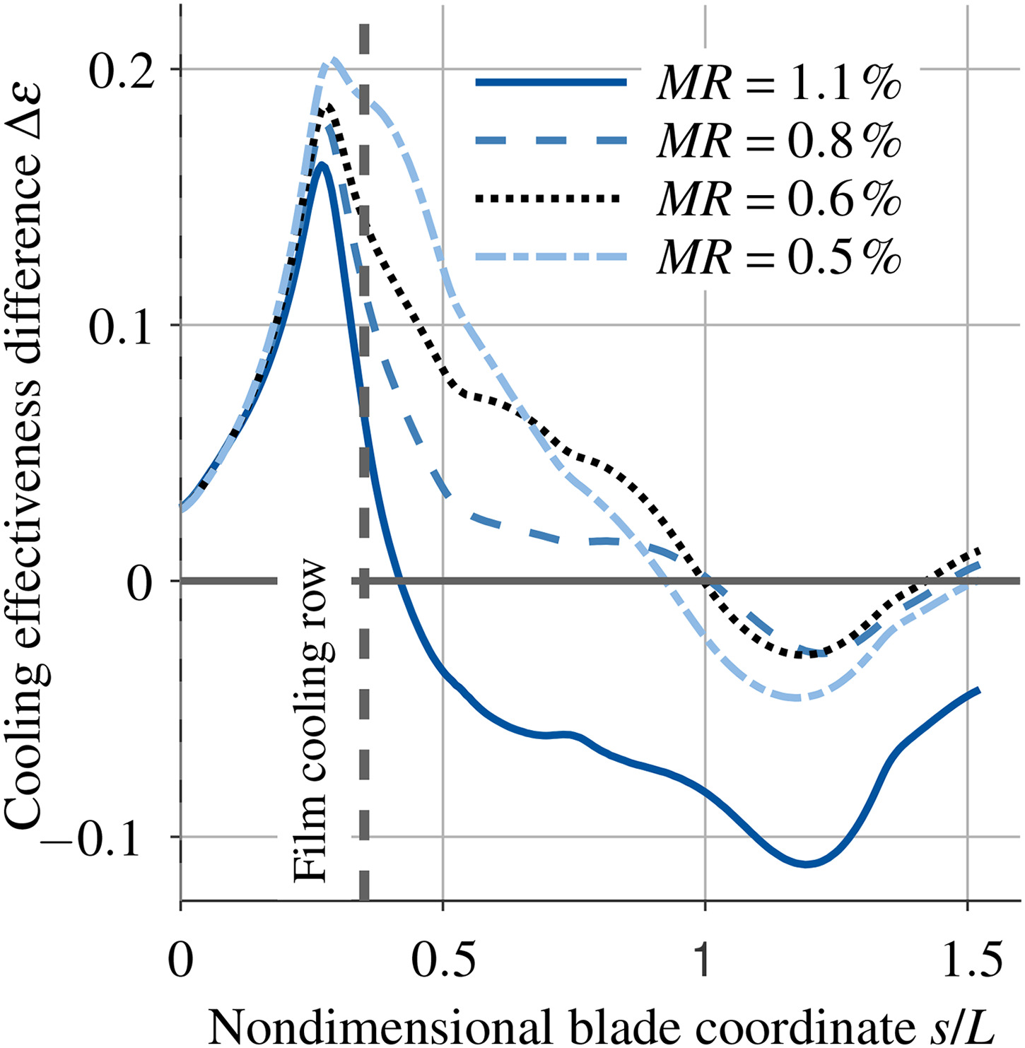
As expected, there is a notable improvement in cooling effectiveness downstream of the film cooling holes in the first region. When the momentum ratio increases however, the improvement gets smaller until the delta effectiveness becomes negative at very high momentum ratios, signifying that the temperature is higher than for the only convectively cooled blade. It is likely that this occurs as a result of the detachment of the cooling jet, which allows hot gas to reach the blade surface and increases the heat transfer coefficient on the blade surface.

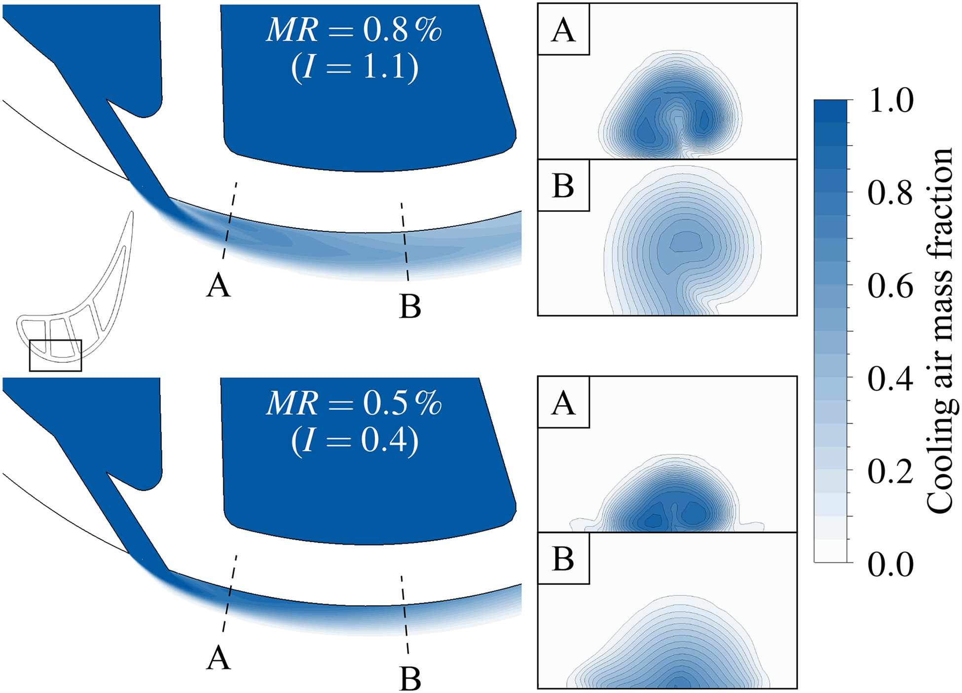
Figure 9 shows contours of the cooling air mass fraction in order to visualize the propagation and structure of the film cooling jet entering the external flow. For the higher momentum ratio of I=1.1, the film cooling jet becomes wider, indicating detachment from the blade surface. This is confirmed in the detailed views A and B oriented perpendicular to the jet. For the low momentum ratio of I=0.4 the cooling air is close to the wall. As the momentum ratio increases, the core of the jet detaches from the wall, resulting in a decreasing cooling effectiveness.

Figure 9.

Cooling air mass fraction of the film cooling jets in the middle plane at two positions perpendicular to the jet at two different MR.

In the intermediate region, the effects are more complicated. The reference mass flow ratio (MR=0.6%) enhances the blade cooling effectiveness significantly, while both higher and lower MR show a lower effectiveness. A higher film cooling mass flow and therefore a higher heat-storage capacity, is beneficial in this region, as long as the film is close to the surface and does not detach. The blade curvature can be favorable here, as long as the momentum ratio is small enough (Ito et al., 1978).

In the mixed-out region, no significant improvement can be observed. For high and low MR, the effectiveness even decreases, which is most likely due to an increased heat transfer coefficient, while the reference ratio and MR=0.8% provide enough heat-storage capacity to compensate for this effect.

Greek symbols

Indices

Latin symbols