
Introduction
In recent years, metric-based mesh adaptation has been gathering significant interest for external aerodynamic flows. This comes as no surprise as in modern Reynolds-Averaged Navier-Stokes (RANS) numerical simulations, the mesh generation and CAD discretization are known as the major bottlenecks that consume significant engineer time that could be better spent exploring more the design space. Recent demonstrations highlighted the ability of mesh adaptation to provide highly accurate predictions on fully unstructured meshes for very complex aircraft geometries (Alauzet and Loseille, 2010, 2016; Park et al., 2018; Alauzet and Frazza, 2021), by reducing and equidistributing the discretization error across the flow domain.
However, mesh adaptation techniques have so far attracted limited interest in the aero-engine community as, traditionally, most aerodynamic RANS simulations of flows inside gas turbines rely heavily on structured multi-block meshes, composed purely of hexahedra (Denton and Dawes, 1998; Arima et al., 1999). Such meshes allow for high numerical efficiency as well as high resolutions in boundary layers and other areas of importance, such as blade wakes. In addition, the considerable industrial experience acquired in the past few decades with such tools has led to extensive calibrations that provide accurate results on standard configurations that contain limited (if any) technological effects.
Such structured meshes do not allow for sufficient local refinement on flow phenomena, such as flow separations, shocks or secondary flows. Additionally, engine manufacturers progress towards more compact and lighter designs, sometimes even with entirely new architectures. Such designs are typically far more sensitive to such flow phenomena as well as to the various technological effects present. Meshing such configurations with structured meshes is practically impossible, hence it is necessary to use unstructured meshes, usually based on empirical meshing strategies for local refinements and the engineer's intuition.
In that context, mesh adaptation techniques appear as a particularly promising way forward to improve the accuracy of RANS predictions for the design of future gas turbines. Different approaches are possible: first, the error estimator for the mesh adaptation can be either computed from a flow variable of interest (“feature based” adaptation) or from the impact of the mesh discretization on an objective output functional (“goal-oriented” adaptation). Second, there are different mesh types that can be used: hexahedral, tetrahedral, multi-element meshes (prisms around the walls, pyramids for transition and tetrahedral everywhere else) or Cartesian meshes with octree refinement (and immersed boundaries). Finally, the mesh adaptation can be either isotropic, to facilitate numerical stability, or anisotropic to follow all the privileged directions of the flow at minimal cost but with numerical difficulties.
Concerning the different configurations of interest for aero-engine manufacturers, there are two main types of flows: internal flows (most notably turbomachinery flows) and hybrid flows that include external aerodynamics in order to study the engine installation effects on its operation. For the former configurations, the limited literature focuses either on mesh adaptation for structured meshes (for example in (Vivarelli et al., 2021)) or isotropic adaptation for multi-element meshes (Wyman et al., 2020). For hybrid external/internal flows, publications focus on unstructured meshes with either limited anisotropy (Ordaz et al., 2017) or with immersed boundaries and octree mesh refinement (Nemec et al., 2019). It is interesting to note that the two different types of flows are practically never treated by the same research groups, with a clear separation of approaches and solvers that are either turbomachinery-oriented or better suited for external flows.
Here a more holistic approach for mesh adaptation, applicable to both types of flows is preferred. It focuses on purely unstructured meshes due to the ease of generation of the initial mesh and mesh adaptation. It also allows a high resolution of boundary layers at an optimal cost (compared to Cartesian meshes with immersed boundaries for example). Recently, we have demonstrated both “feature-based” and “goal-oriented” tetrahedral anisotropic mesh adaptation on turbomachinery test cases using the vertex-centered solver Wolf (Alauzet et al., 2021), which was developed for handling highly anisotropic elements. In this work, we demonstrate mesh adaptation on a hybrid type of flow: a nacelle under crosswind conditions, leading to inlet distortion. The focus is on “feature-based” adaptation but on two types of meshes: pure tetrahedral meshes with anisotropic adaptation and multi-element meshes with isotropic adaptation. As with our previous work, the former is resolved by the vertex-centered, compressible solver Wolf. The latter approach is combined with the cell-centered, compressible solver elsA, a more standard solver, typical of CFD software used in the aero-engine community today.
The objective of this paper is twofold: (1) demonstrate the abilities of unstructured body-fitted mesh adaptation in this complex flow, characterised by flow separation, hysteresis and low overall Mach number, with both standard and more advanced numerical approaches and solvers and (2) compare between the typical multi-element meshes with isotropic tetrahedra, commonly used in the industry today, with highly anisotropic tetrahedral meshes provided by the mesh adaptation algorithms. The selected test case is supplied with some experimental data and a reference “one shot” unstructured simulations using standard meshing practices.
Test case
The considered test case in this work is the nacelle MASCOT2. It is a research nacelle whose geometry was designed to be representative of a short nacelle for high bypass ratio engines. It is not an axisymmetric nacelle but it has a vertical symmetry across the y-axis. Different versions of this geometry exist: (1) with separated primary flow/bypass paths or with a single engine path combining both and (2) with or without the presence of a fan. Here, the simplest configuration is employed: a single flux nacelle without the presence of fan, as it is the version that was experimentally tested for inlet distortion under crosswind conditions in the F1 wind tunnel of ONERA (Sadoudi, 2016) (Figure 1).
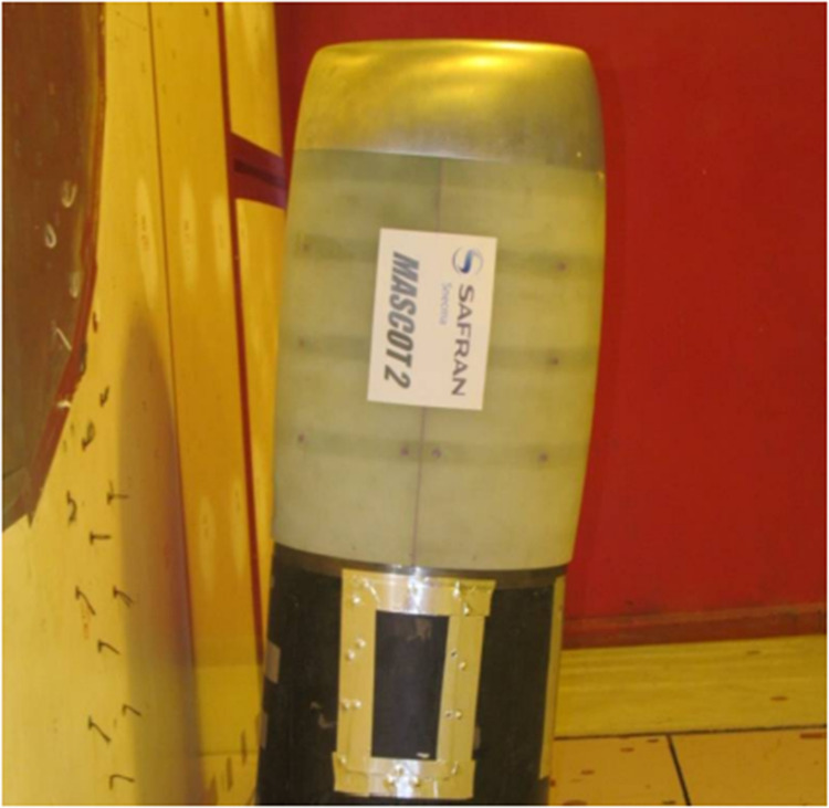
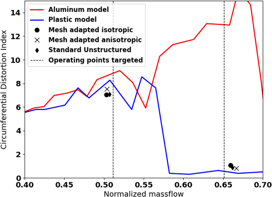
Two different experimental configurations were measured: one where the front of the nacelle was manufactured from aluminium and one from plastic using rapid prototyping. Both configurations have the same plastic cowlings further downstream. During the testing, it was realized that the different experimental configurations experienced important differences of their respective distortion index, with the aluminium case showing the subsonic distortion continuing at significantly larger massflows before the reattachment zone (Figure 2). This is attributed to the different tolerances between the two cases (0.08 mm for the aluminium case vs 0.4 mm for the plastic case), as the flow separation at this flow regime close to reattachment is particularly sensitive to geometric variations. It is also worth noting that the flow at this regime is known to experience a hysteresis phenomenon, where the flow can be attached or separated depending on the initial condition of the simulations (Colin, 2007). This is of particular importance as will be shown later.
Figure 2.
Experimentally measured Circumferential Distortion Index (CDI) for the two models and operating points targeted.
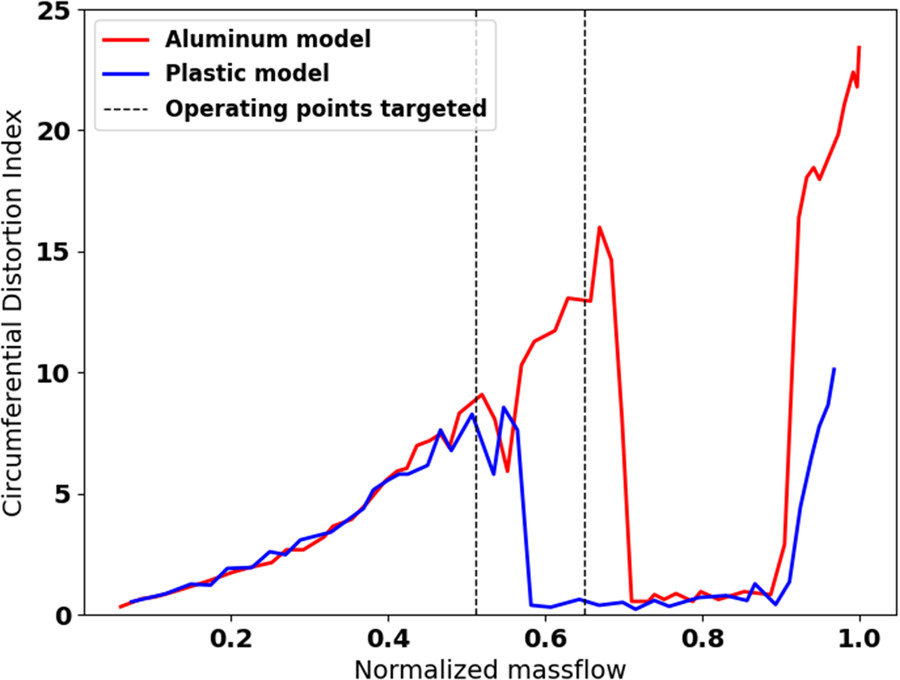
In this work, two different operating points were simulated, both located in the subsonic separation region of the operation of this nacelle under crosswind conditions (highlighted by the vertical dash lines in Figure 2). Both points are located relatively close to the reattachment region. The choice of these operating points was due to the sensitivity of the flow at this regime.
Numerical setup
The numerical methods and setups used in the paper are presented below.
Meshes
As mentioned in the introduction, in this work we employ various meshing strategies to evaluate the performance of different mesh adaptation approaches and their impact compared to the standard “one shot” simulations. As a result, three different types of meshes are used in this work:
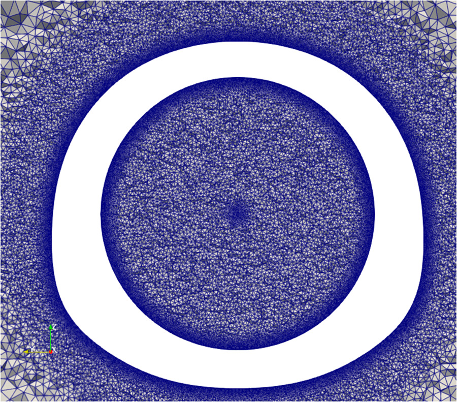
A typical unstructured multi-element tailored mesh that is generated manually with a standard empirical approach using ANSA mesh generator to serve as a reference to the current practices. This mesh consists in isotropic tetrahedra and prism layers around the nacelle, in the boundary layer region. Various refinements around the nacelle are included to account for the expected separation. The mesh contains 98M elements. A view of this mesh is provided in Figure 3.
Adapted isotropic multi-element meshes: meshes that result from mesh adaptation on the features of the flow and include isotropic tetrahedra in the main field and extruded prism layers from the nacelle's surfaces. The maximal mesh size in this work is 54M cells.
Adapted anisotropic tetrahedral meshes: tetrahedral meshes that result from mesh adaptation on the features of the flow but without enforcing isotropy on the elements. This implies that the adaptation is free to determine the optimal form of the tetrahedra in order to follow the preferential directions of the flow for an imposed number of vertices in the mesh. The maximal vertex count of the anisotropic meshes is 5.5 M vertices.
On the other hand, the reference unstructured multi-element mesh required approximately 1 h, in order to set-up the necessary local refinements and generate the multi-element mesh. This time assumes that there is no additional intervention by the user after the CFD run, in an effort to improve the mesh and refine further in certain areas or to evaluate the mesh convergence of the simulations, which is frequently the case. Additionally, the difference between the two approaches is expected to be even bigger for more complex geometries, where manual refinements become even more laborious compared to the generation of basic coarse tetrahedral meshes.
Solvers and numerical parameters
The unstructured multi-element reference mesh or mesh-adapted isotropic simulations are performed with the elsA solver. elsA is a cell-centered (flow variables are stored at the center of mesh elements) finite volume discretization CFD solver developed by the ONERA (Cambier et al., 2011; Cambier et al., 2013) that can work with structured, unstructured or hybrid meshes. The standard form of the turbulence model of Spalart and Allmaras turbulence model is used (Spalart and Allmaras, 1992), without wall functions. The spatial discretization relies on the upwind Roe scheme, in conjunction with the limiter of Venkatakrishnan (Venkatakrishnan, 1995), achieving second order accuracy. A first order backward-Euler algorithm is used for time-marching, using an implicit formulation.
The anisotropic mesh-adapted simulations are performed with the Wolf solver. Wolf is a vertex-centered (flow variables are stored at vertices of the mesh) mixed finite-volume – finite-element Navier-Stokes solver on unstructured meshes composed of triangles in 2D and tetrahedra in 3D. The convective terms are solved by the finite-volume method on the dual mesh composed of median cells. It uses the HLLC approximate Riemann solver to compute the flux at the cell interface. Second order space accuracy is achieved through a piecewise linear interpolation based on the Monotonic Upwind Scheme for Conservation Law (MUSCL) procedure which uses a particular edge-based formulation with upwind elements (Alauzet et al., 2021). As with elsA, a backward Euler time-integration scheme is used, with the addition of local time stepping to accelerate the convergence to steady state. Likewise the turbulence model of Spalart and Allmaras is used without wall functions.
The CFD runs continue until convergence of the massflow for the elsA runs (variation of the massflow less than 0.5%), which also includes convergence of the residuals by 4 orders of magnitude, and until convergence of the residuals by 6 orders of magnitude for the Wolf runs.
Domain and boundary conditions
The domain consists of a large box that englobes the nacelle under study. The external surfaces of the nacelle are prolonged to reach the back of the box, similarly to the experimental configuration. Inside the nacelle, the surfaces arrive at an outlet condition that simulates the aspiration of the flow by the engine. The domain and boundary conditions are represented in Figure 4.
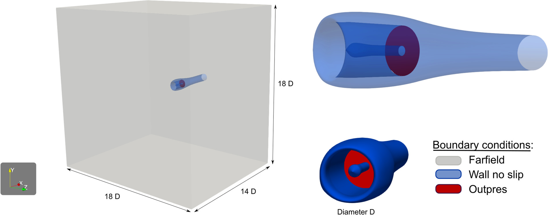
Concerning the boundary conditions, the same conditions and values are imposed for all simulations to ensure coherence between the comparisons. First, farfield conditions are applied at the outer surfaces of the box, with 25 kt of crosswind velocity imposed. Wall no-slip conditions are imposed on all nacelle surfaces. Finally, at the outlet condition that models the engine aspiration, a constant static pressure is imposed, 95 kPa for the first operating point and 90 kPa for the second.
Adaptation workflows
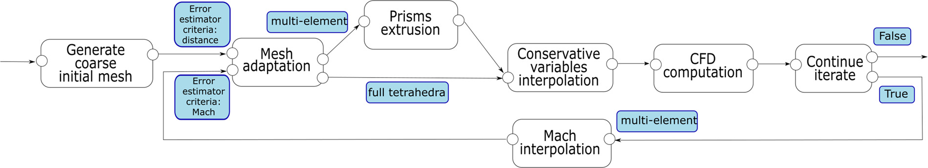
Two different meshing strategies have been evaluated in this work, each with a respective workflow. The first is isotropic multi-element adaptation, capable to function with the typical solvers used in the industry. The second is an anisotropic tetrahedral-only adaptation, which requires solvers specifically tailored for such meshes. An overview of the global mesh adaptation workflow is provided in Figure 5.
Isotropic multi-element workflow
Adaptation process
From a mesh, a criteria field on this mesh, as well as a user-imposed number of elements, an isotropic mesh adaptation process using the remesher of Inria, feflo.a (Loseille and Löhner, 2013), is performed. The Mach flow field is chosen as the relevant criterion to adapt the mesh on the physics of the flow such that the mesh is refined on Mach variations, using the error estimator described in (Alauzet et al., 2021). The remesher will use the number of elements as a constraint. Then, prism layers are extruded from the walls, crushing the tetrahedral mesh, using bloom (Alauzet and Marcum, 2015). Next, the conservative variables from the previous solution are interpolated to the new multi-element mesh and the elsA computation is launched. The Mach solution from this new elsA computation is then interpolated on the previously adapted tetrahedral mesh, and the remeshing process can be run again.
In practice
The initial mesh is a coarse mesh with no user refinement zone, so that it can be generated with no user effort with ANSA. Then, a first adaptation is run on the inverse of the distance to the walls. This stage is important for elsA solver as it generates a first mesh with a smooth size transition and finer mesh close to the walls. It ensures that the first CFD run is a good approximation of the solution. Then 5 remeshing process are done with an imposed number of elements of 8 M, and 5 additional ones with an imposed number of elements of 16 M. These computations are done with the cell-centered elsA solver so the number of elements correspond to the degrees of freedom (DoFs).
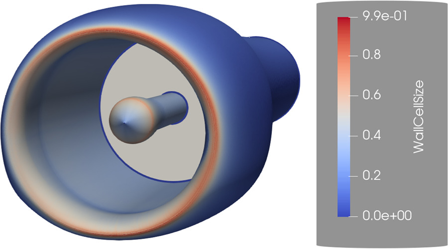
Note that prism layers are not included yet in the DoFs count. After each tetrahedral remeshing, 40 layers of prisms are generated from the walls with a first cell mesh size of 3e-6 m to ensure y+ < 1 on the wall. The resulting y+ over the nacelle after computation is presented in Figure 6.
Moreover, for tetrahedral adaptation, the growth rate is specified to 1.2 and tetrahedra are limited to a size under 1.5 m. An overview of the parameters, and resulting vertex and element counts is provided in Table 1.
Anisotropic tetrahedral workflow
Anisotropic mesh is a promising alternative to prism layers, as it is more straightforward to implement, efficient and can be more robust. It allows to have elements stretched in the flow direction and very fine in the other directions to follow the preferential directions of the flow, reducing the total number of tetrahedra needed. To obtain accurate solutions on this type of meshes, a vertex-centered solver with classic numerical schemes, like the solver Wolf used in this work. This workflow is lighter than the isotropic one as the prism extrusion is skipped.
In practice
As this workflow does not have the considerable additional cost of prisms layer, it can be run with several more refinement level, as detailed in Table 2, allowing to have a better idea of the global convergence of the process.
Moreover, for tetrahedral adaptation, as the solver is more robust on stretched elements, the growth rate is specified to 1.4 and tetrahedra are limited to a size under 5 m. The y+ on the wall is not manually controlled, it is the error estimator which evaluates the best mesh size. Post-processing of the y+ on the walls, showed that it is under 8 around all walls. An overview of the parameters, and resulting vertex and element counts is provided in Table 2.
Results and discussion
Convergence of the mesh adaptation processes
Before evaluating in detail the results of the numerical simulations, it is necessary to determine the overall convergence of the isotropic and anisotropic mesh adaptation processes. This will allow to establish if the simulation results have stabilized at the end of the adaptation process. To evaluate the overall convergence, the most pertinent value for this type of flows is the Circumferential Distortion Index (CDI) (Gil-Prieto et al., 2018). Figures 7 and 8 depict the CDI for the multi-element isotropic and tetrahedral anisotropic processes, respectively. As the cost of the CFD runs with isotropic adaptation is considerably larger than the anisotropic one (due to the large number of prisms around the nacelle added), only two refinement level have been used, the x-axes of Figure 7 are the adaptation cycle for clarity. On the other hand, with the anisotropic process we perform several more cycles in lower mesh size and more mesh sizes are evaluated. As a result, the x-axes in Figure 8 are the number of vertices, with the CDI of each run indicated by a dot and the final run of each refinement level linked with a line, to show the final results. The CDI of the experimental measurements is also depicted for comparisons.
Figure 7.
Evolution of the CDI for the isotropic mesh adaptation cycle, first operating point (top) and second operating point (bottom).
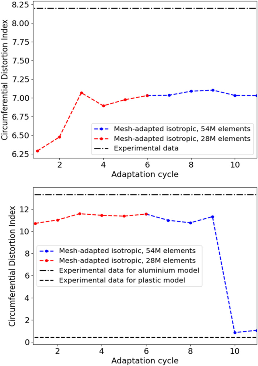
Figure 8.
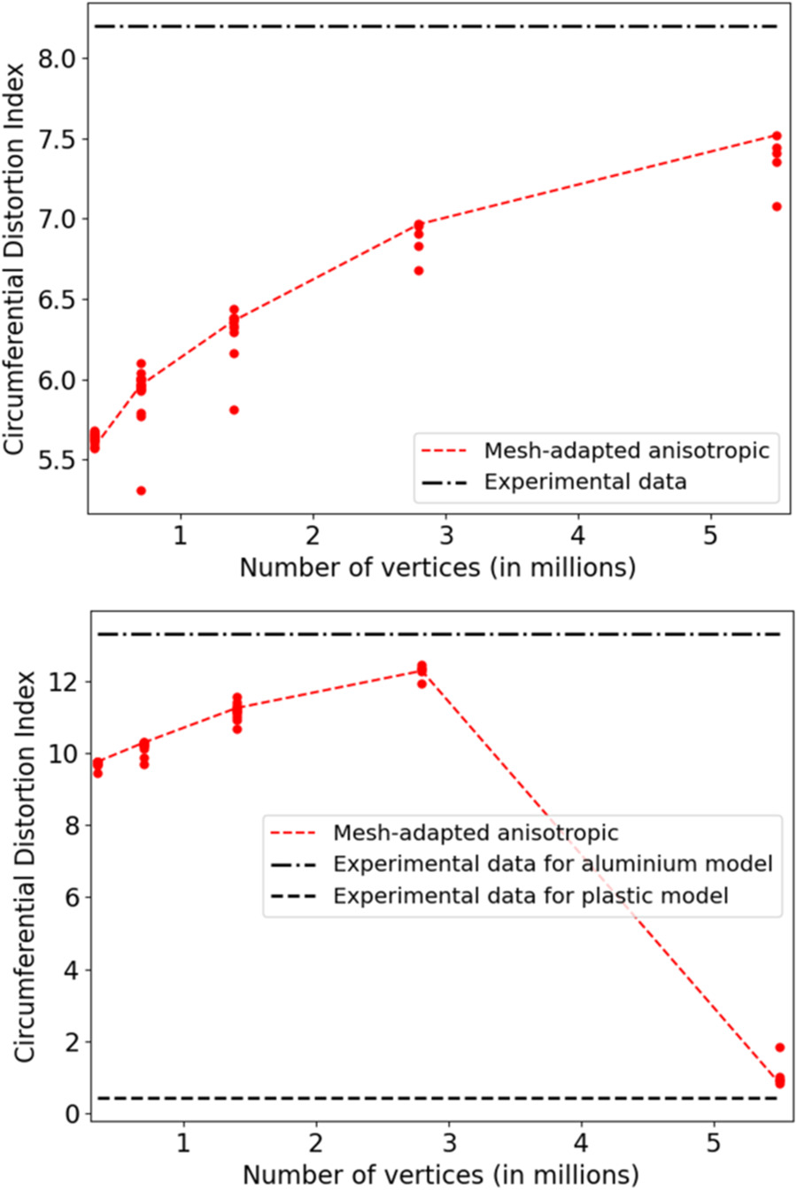
Evolution of the CDI for the anisotropic mesh adaptation process as a function of the number of vertices, first operating point (top), and second operating point (bottom).
Concerning the convergence of the isotropic multi-element adaptation process, Figure 7 presents the results of the CDI for each CFD run, and for two operating points. The results for the first refinement level with 28 M elements are depicted in red while the results for the second refinement level with 54 M elements are depicted in blue. For the first operating point, Figure 7 (top), we can see that for the first refinement level the CDI oscillates around 7% after the first couple of runs. Switching to the second refinement level, the CDI becomes stabilized with only minor variations between runs and staying within approximately 1% of the experimental CDI value. This indicates that the process appears converged and some more runs on the first refinement level could likely have been sufficient. The second operating point is very interesting as there are two different results for the CDI, depending on the type of the geometry model (aluminium or plastic). One can observe in Figure 7 (bottom) that no matter the number of elements until the tenth adaptation cycle, the CDI converge to a value similar to the aluminium model. However, from the tenth cycle, the CDI decreases to the plastic model solution which is a very stable solution with no distortion present.
Concerning the convergence of the anisotropic adaptation process, Figure 8, presents the results of the CDI for each CFD run and for the two operating points. For the first operating point, Figure 8 (top), we can see that there is a relatively small dispersion between each run for each refinement level, with only a couple of outliers (mainly for the coarser meshes) and then a relatively quick convergence to the final value. As the mesh gets refined, the CDI gradually increases but with a reduced slope after each increase in mesh size. This suggests that the process is reaching an overall convergence, with a final CDI value close to the one predicted experimentally. However, some additional runs at the next refinement level (11M vertices) appear necessary in order to achieve a complete convergence, likely approaching the experimental value further. For the second operating point, Figure 8 (bottom), there is a similar trend up to the second-to-last refinement level, reaching high CDI values that correspond to the distortion depicted by the aluminium model experimentally. However, at the last refinement level, the CDI drops dramatically, implying the suppression of the inlet distortion, similar to the behaviour of the plastic model. This behaviour confirms the very high sensitivity of the prediction at this operating point: even the small differences in the discretization of the geometry induced by the mesh adaptation process suffice to change the overall flow field.
Analysis
The first point to be evaluated for the different numerical predictions is the final CDI, for both operating points, versus the experimental measurements. This is depicted in Figure 9. As it can be readily observed, both mesh-adapted solutions (isotropic and anisotropic) are very close to the experimental values and to the standard unstructured mesh predictions, with the anisotropic mesh adaptation results being slightly ahead to the other predictions. Regarding the second operating point in particular, all simulations follow the predictions of the plastic model with practically no inlet distortion. These findings suggest that (1) the mesh adaptation processes lock on the right flow physics, providing reliable predictions and (2) the plastic model seems to correspond better to the numerical setup for this configuration. However, the availability of the global convergence progress provided by the mesh adaptation process, provides here additional information compared to standard one-shot simulations: the high CDI values predicted (closely matching the aluminium model) that suddenly decrease with mesh refinement can be a good indication to the designer for the sensitivity of the flow in this particular area of operation.
Figure 9.
CDI comparison between the different numerical predictions and the experimental measurement.
Having looked at the global CDI predictions, we now turn to a more qualitative analysis of the flow field and the resulting meshes. Figures 10 and 11 present the stagnation pressure at an axial cut (that corresponds to the position where the fan is normally found) and the resulting mesh for the two different mesh adaptation processes and for the two operating points respectively. The stagnation pressure for the standard unstructured prediction, from the manually generated mesh that serves as the reference to standard industrial practices, is also provided.
Figure 10.
Mesh view and pressure stagnation at an axial cut for the first operating point. Isotropic mesh adaptation (top), anisotropic mesh adaptation (bottom), standard unstructured simulation (right).
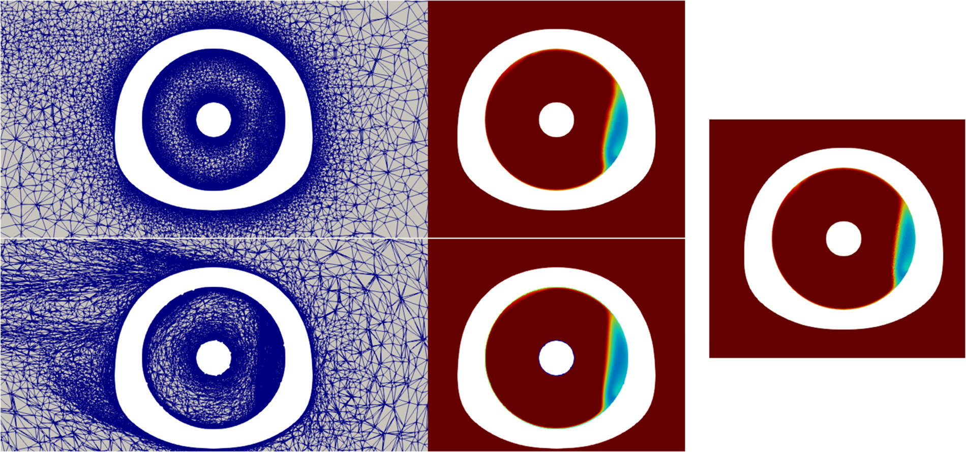
Figure 11.
Mesh view and pressure stagnation at an axial cut for the second operating point. Isotropic mesh adaptation (top), anisotropic mesh adaptation (bottom), standard unstructured simulation (right).
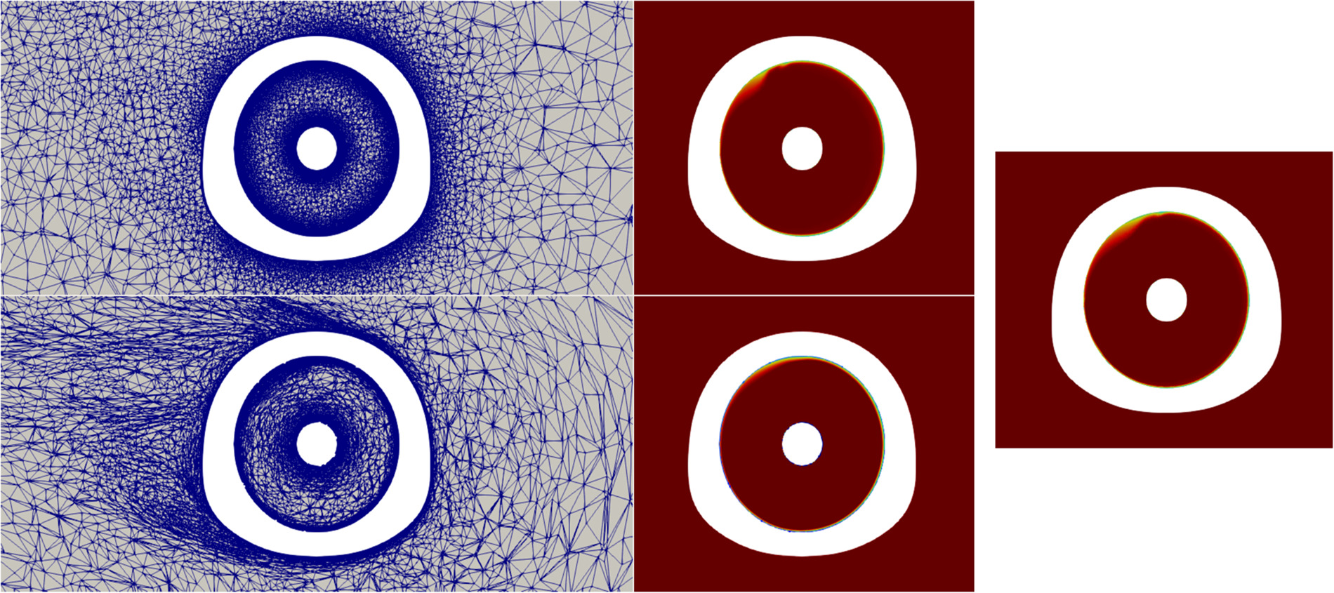
The first thing that can be easily concluded, for both operating points, is the similarities between the different numerical predictions. For the first operating point, Figure 10, all simulations predict a very similar distortion, both in size and in amplitude. The most noticeable difference is that the distortion of the anisotropic mesh adaptation prediction appears slightly larger closer to the top of the engine. For the second operating point, Figure 11, there is practically no visible distortion, with only a very small distortion at the top left from flow ingested close to the wake of the nacelle. These findings confirm indeed that the mesh adaptation captures the expected flow physics. They also highlight that the omission of prism layers in the anisotropic adaptation does not appear to deteriorate the results and the adaptation itself leads to meshes that resolve sufficiently the boundary layers. This confirms the observations of (Alauzet et al., 2021) on a turbomachinery test case and illustrates that very important gains in computational cost can be obtained by highly anisotropic adaptation, as the number of degrees of freedom dramatically reduces (here 5 M DoFs versus the 50+M DoFs for the multi-element isotropic approach or the almost 100 M DoFs of the standard unstructured mesh) and the time required for the prisms extrusion is no longer necessary.
Looking now at the mesh views, several interesting points can be observed. First, the mesh adaptation correctly refines the boundary layers and particularly the boundary layers within the engine inlet. This is normal as the aspiration by the engine accelerates the slow external flow (the crosswind is only 25 kt) and thus leads to finer boundary layers within the engine with stronger gradients. Second, in Figure 10 where an inlet distortion is predicted, both mesh adaptation processes refine around the distortion: a more moderate refinement for the isotropic process and a strong refinement for the anisotropic process. The difference in the intensity of the adaptation is readily attributed to the mesh adaptation approach: anisotropic adaptation allows to follow the shear layers with fewer cells, thus enabling higher refinement at reduced counts of DoFs. Finally, the last difference is on the refinement of the wake generated by the crosswind as it impacts the nacelle. The isotropic adaptation shows practically very limited refinement. On the other hand, the anisotropic adaptation, with its optimal precision for a given cost, allows to also refine this area. This is of little impact for this type of flows where only the prediction of the inlet distortion is desired. However, the overall flow field behaviour in the domain can be important in other studies, such as those that investigate engine installation effects.
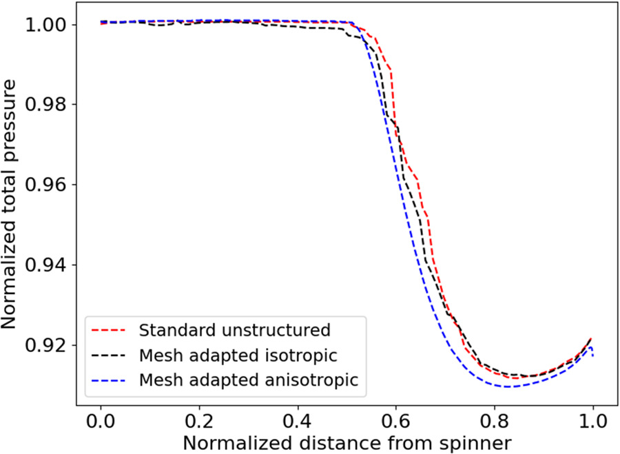
Finally, in order to get a more quantitative view of the inlet distortion between simulations, Figure 12 presents the normalized total pressure profiles for the different numerical predictions across a radius from the spinner to the nacelle at 180 degrees (z = 0). As expected, only minor differences between the simulations are observed both on the total pressure amplitudes as well as the form. It can also be noted that the curve of the anisotropic mesh-adapted results is smoother, highlighting the additional refinement afforded by the approach.
Computational cost
After analysing the results, some information on the cost of the mesh adaptation processes is provided below.
For the isotropic mesh adaptation:
Adapting the tetrahedral mesh is very quick, taking less than 5 min
The prism extrusion is the longest part of the mesh manipulation part, taking approximately 20 min
The CFD runs are, as expected, the most time-consuming part of the process: for the first refinement level around 10 h on 200 CPU cores (Intel Cascade Lake) per run are necessary and for the second refinement level around 17 h on 200 CPU cores per run.
The standard unstructured simulation required approximately 1.5 days on 240 CPU cores for full convergence.
These numbers highlight that from a purely computational cost perspective, the mesh adaptation process is more costly today and that the main gains are primarily in user time and precision. This implies that the engineer no longer needs to spend large amounts of time generating or refining meshes and can instead spend more time investigating the design space while the mesh adaptation process automatically minimizes the discretization error. However, with MPI-capable anisotropic adaptation, it is likely to also achieve a cost-competitive process compared to the typical one-shot simulations that are prevalent in the industry today.
Conclusions
In this work, two different strategies of feature-based mesh adaptation were evaluated on a nacelle under crosswind conditions test case: isotropic, multi-element adaptation and anisotropic tetrahedral adaptation for two different operating conditions. The main findings have been that:
Both approaches provided accurate predictions of the flow field, starting from a very coarse tetrahedral mesh
The anisotropic mesh adaptation manages to achieve similar accuracy at only a tiny fraction of the total DoFs count (1/20th of the total DoFs of a typical unstructured mesh)
Both mesh adaptation processes showed an abrupt change of the flow behaviour for the second operating point evaluated as the process proceeded towards global mesh convergence, exhibiting the sensitivity of the flow observed experimentally.
Mesh adaptation greatly alleviates the bottleneck of mesh generation
While the computational cost of mesh adaptation is today more expensive compared to one-shot simulations, it is highly probable that in the future anisotropic mesh adaptation can become competitive.