
Introduction
Characterizing the aerodynamic performance of airfoils has been based since decades on measuring the total pressure losses in the wake of the aeroshape using pressure probes, such as pitot, preston or multi-hole tubes (e.g., five-hole probe - 5HP), compare (Truckenmüller and Stetter, 1996; Börner et al., 2018). These probes are used at the location of interest, where either a single probe is traversed along a specific path or a probe rake at several locations simultaneously provides information about the distribution of the total pressure downstream of a flow body. The flow conditions in jet engines cover nearly all ranges from low-speed to supersonic Mach number conditions at Reynolds numbers from
The pressure field is a fundamental property of fluid flow, governing important phenomena such as fluid forces, energy transfer, and flow stability. Direct measurement of pressure is often challenging, especially in complex and dynamic flow environments. Particle Image Velocimetry (PIV) has emerged as a powerful experimental technique for quantifying fluid flow fields in various engineering applications. By capturing images of particles in seeded flows illuminated by laser light, PIV enables researchers to obtain velocity vector fields with high spatial and temporal resolution (Adrian and Westerweel, 2011; Raffel et al., 2018). While velocity information is crucial for understanding flow dynamics, the derivation of pressure fields from PIV data is equally important for comprehensive flow characterization and analysis. In recent years, the hardware development as well as the derivation of computational methods enabled the calculation of pressure fields derived from PIV based on different numerical approaches and boundary conditions, Charonko et al. (2010), van Oudheusden (2013), van Gent et al. (2017), and Tagliabue et al. (2016). Consequently, there has been considerable interest in developing techniques throughout various fields of application to infer pressure fields from velocity data obtained via PIV measurements, Ragni et al. (2009), de Kat et al. (2009), and Jacobi et al. (2022). These methods can be broadly classified into two categories: inviscid and viscous formulations. For inviscid formulations, the pressure field is obtained by solving simplified versions of the Navier-Stokes equations, neglecting viscous effects.
The application of the presented approach to viscous and even non-adiabatic flows is also part of the present research, even knowing that compromises in terms of accuracy are requisite, see e.g. van Oudheusden (2008). On the other hand, viscous formulations aim to account for the influence of viscosity on the flow field by solving additional equations or imposing constraints based on physical principles. Common approaches include the Navier-Stokes equations with appropriate boundary conditions, integral methods such as the pressure Poisson equation, and optimization-based techniques utilizing velocity and continuity constraints.
Both these well-established experimental approaches (5HP and PIV) will be merged within this paper, which aims to deliver a practical approach for the estimation of total pressure losses in wake-dominated flows such as individual airfoil or cascade exit flows. Initial work which deals in particular with cascades operating at non-adiabatic conditions but which is based on CFD data has been presented by Rusted and Lynch (2021). In this paper, a hybrid approach is used combining local but accurate total pressure measurements and reconstructed pressure fields from PIV into a plausible total pressure field. Its high spatial resolution may be advantageous in investigating wake-dominated flows. The remainder of this report is organized as follows: The testcase and the methodology for collecting the experimental data with pressure probe traverses and PIV is presented in the section Methodology. The hybrid approach is presented and validated in the subsequent sections. Finally, the approach is applied to a low-pressure turbine flow field in the last section.
Methodology
The aim of this paper is to provide a practical and at the same time widely general approach that enables the determination of total pressure losses of aerodynamic test specimens - both, with high spatial resolution at descent measurement accuracy. It must be clearly stated that the authors are aware that for the aim of accurately determining local and integral total pressure losses from measuring the vessels’ ambient reference pressure
Table 1.
Aerodynamic reference values at operating points and boundary conditions for pressure calculation in DaVis; the reference length for R e D D = 10
the choice and combination of measurement methods presented here is inferior to the highly accurate established methods, such as e.g., five-hole probes (5HP), as discussed in Truckenmüller and Stetter (1996), Hoenen et al. (2012), and Börner et al. (2018). However, assuming a slightly reduced accuracy is accepted, the presented approach offers enormous added value with regard to the spatial resolution of the reconstructed pressure fields in particular for the analysis of complex flow fields, such as they can occur in linear blade cascades operating at transonic conditions. Such cascade flows are usually extensively qualified in the High-Speed Cascade Wind Tunnel (HGK) at the University of the Bundeswehr in Munich. On the one hand, the presented approach is intended to expand the offered portfolio of measurement techniques and, to enable more in-depth aerodynamic analysis of complex flow processes on the other hand.
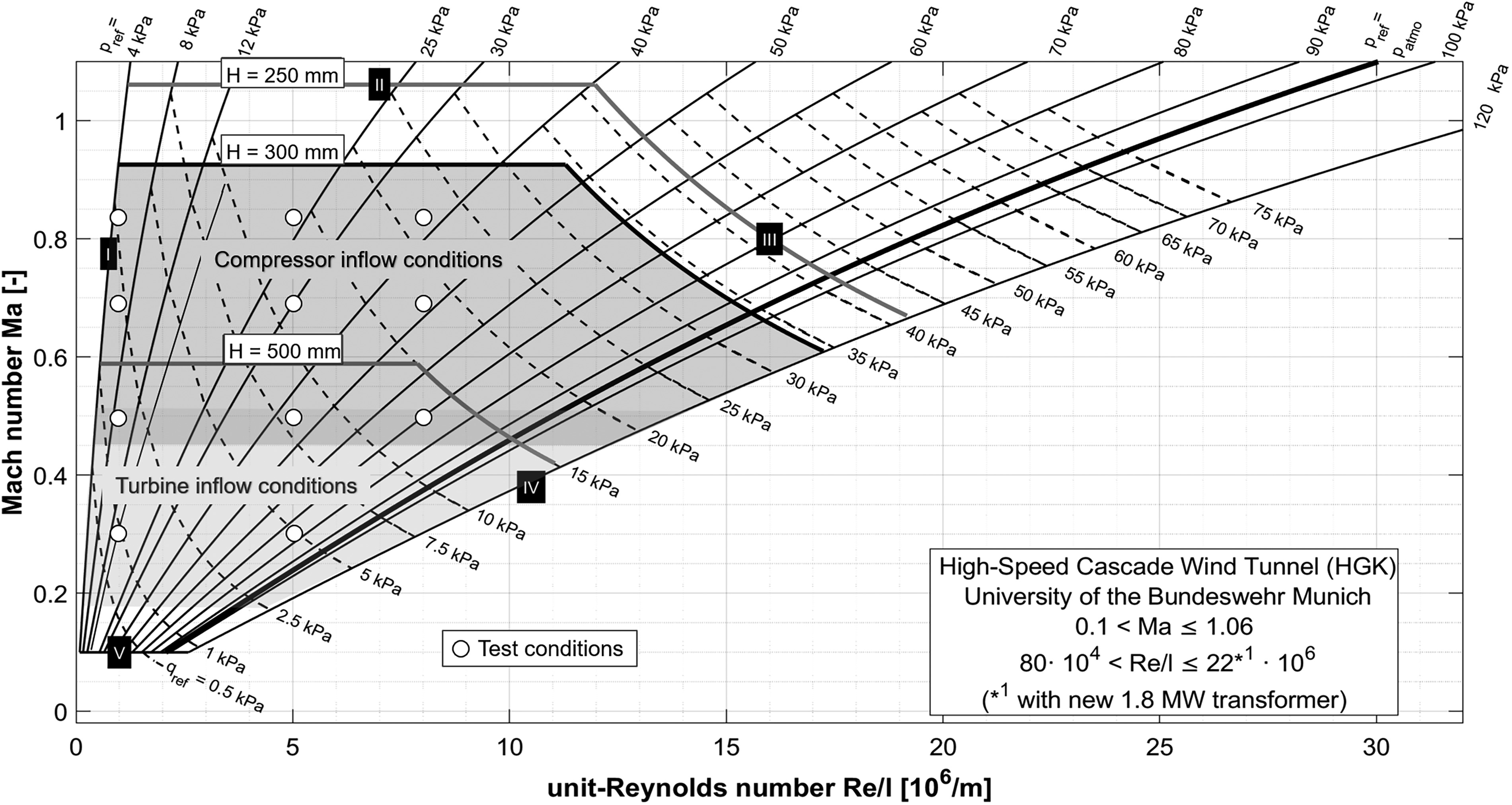
The HGK is a continuously operating wind tunnel, which enables experimental investigations of turbomachinery bladings under engine-relevant flow conditions (Mach and Reynolds numbers, turbulence intensity), see Niehuis and Bitter (2021). The operating map of the test facility is shown in Figure 1. The wide range of Mach and Reynolds numbers is enabled by the fact that the ambient pressure in the test facility can be varied between
Figure 1.
Aerodynamic operating conditions of the High-speed Cascade Wind Tunnel Munich, adapted from Niehuis and Bitter (2021). Tested operating points are labeled with ∘ p r e f p r e f
A cylinder in crossflow (
Figure 2.
Left: Upstream view towards the cylinder mounted on the flat plate at the test section outlet of the HGK. The PIV Laser plane as well as the probe traverses were positioned z = 30

Pressure measurements
A probe rake comprising a pitot tube, a static pressure tube and a hot-wire probe for measuring turbulence spectra (discussion is not part of this paper) was traversed in the cylinder wake. The pitot pressure probes’ head had an outer diameter of 1.2 mm and an inner diameter of 0.8 mm. Traversing was performed from
The probe pressure data was acquired using differential pressure transducers in a rack-mount pressure scanner 98RK-1 from Pressure Systems Inc. offering a pressure range of
PIV measurements
The general plausibility of applying particle-seeded flow diagnostics to turbomachinery flows and in particular in the HGK environment which partly operates at the density limits of the Stokes-flow conditions, was investigated in e.g., Ruck (1990) and Engel (2007) or Bitter et al. (2016). The particles’ following behavior is widely sufficient for flows down to static pressure levels of
The PIV laser plane was introduced into the test section from the far wake behind the cylinder. An Innolas Spitlight 1000 Nd:YAG double-frame laser provided 480 mJ optical power per pulse to illuminate the particles in the field. A scientific CMOS camera with double-shutter option was installed at a distance of 500 mm away from the laser plane. The camera was equipped with a 35 mm Zeiss macro lens to capture a field of view which even slightly extends the dimensions from the probes’ field traverse. The field of view was calibrated with a planar calibration plate which was manually aligned with the flow field and the laser plane with an angular accuracy of better than 0.1 degree. The calibration scheme which is based on a second order polynomial as implemented in DaVis was applied for image reconstruction.
The flow was seeded with DEHS particles of
In order to ensure fully-converged Reynolds stress fields which are required for the application of the RANS equation in the pressure reconstruction scheme, 5,000 PIV images were captured and analyzed at each operating point. PIV data evaluation was performed with LaVisions’ latest release of the commercially available state-of-the-art PIV software Davis 10. An iterative window-based cross-correlation approach which is standard approach for PIV evaluation was applied. The vector field of each PIV snap-shot was individually calculated based on a reducing interrogation window size (IWS) from 96 px down to 48 px at 75 %. From the authors’ experience, this is a good compromise between spatial resolution and vector field calculation accuracy as a consequence of the particle density. The final PIV field had a spatial vector density of 0.46 mm/vector, which is about 8–10 times higher compared to a classical pressure probe traverse. Data post-processing and moderate spatial interpolation was applied in cases where required. Both, the data availability and vector validity were better than 99% for the cases of
Pressure reconstruction approach
The PIV software (LaVision, 2021) enables the reconstruction of the pressure field from both, instantaneous and time-averaged PIV velocity fields. Since this paper focusses on the presentation of a practical hybrid approach and the deeper assessment of the RANS-based reconstruction scheme can be found in e.g., Charonko et al. (2010), van Oudheusden (2013) or van Gent et al. (2017), the authors will skip the discussion at this position. Latest work by Nie et al. (2022) investigate major impact factors caused by PIV fields and propagate into the reconstructed pressure field.
It must be stated, that several restrictions between the implemented method in the software and the proposed application in the hybrid approach presented here, apply. Mainly, the algorithm expects an incompressible Newtonian fluid (e.g., water and air) where the density and dynamic viscosity of the working fluid are assumed to be constant. Secondly, the RANS equation requires the Reynolds stress fields to be fully-converged. The latter one can be encountered by providing a sufficiently high number of snapshots used for averaging as provided in this work. A discussion of losses and drawbacks of the first statement can be found in van Oudheusden (2008) where the pressure reconstruction method is applied to compressible high-speed flows.
Together with the marching scheme, the proposed boundary conditions are crucial for the accuracy of the reconstructed pressure field. Unless otherwise available, global static pressure values must be used for the Dirichlet condition. But, if available, the pressure distribution along a path or across a surface can serve as boundary condition, compare e.g. Tagliabue et al. (2016). The Hybrid PPA: Hybrid Probe - PIV - Approach for Pressure Reconstruction will be demonstrated and validated in the following, comprising from the following steps:
Provide total pressure information of a flow field at discrete reference points all over the field of interest,
Provide a statistically converged PIV vector flow field which also covers the reference points in the same field of interest.
Apply the following procedure for the reconstruction of the pressure field from PIV by using commercially available PIV software: 0. Select a valid PIV velocity field at a corresponding operating point; 1. Set a working fluid –> air with viscosity and reference density according to the operating point from Table 1; 2. Set the solver options to time-averaged pressure reconstruction; 3. apply a global average pressure boundary condition; 4. compute the pressure field.
Convert the static pressure field from 3) into a total pressure field by means of the isentropic conversion as given in Equations 3 and 4, whereas
Use the reference point(s) from 1) to perform a polynomial in-situ correction of the calculated pressure field from 4) and evaluate the fit all through the PIV field.
Validation and discussion
The approach is designed to work generally if any valid PIV flow fields together with corresponding pressure data at reference positions in the field are available. The decision for a proper experimental PIV setup has than already been made following the general guidelines and common procedures as given by standard literature. The following section presents the validation and discussion of the approach as it was developed by using the cylinder data set. This section is followed by the discussion of the approach for total pressure loss estimation in the wake flow field of a linear low-pressure turbine (LPT) cascade.
Cylinder in crossflow
The results presented in this section are based on the 5 steps introduced in the previous chapter. The raw pressure fields, as they were calculated with LaVision (2021) by applying the outlined procedure from the previous section, serve as the starting point for further discussion. Beyond this initial discussion, only the fitted/corrected pressure data is discussed in the context of the paper. First, the raw reconstructed pressure data from PIV will be compared to classic probe-based total pressure measurements for Mach numbers ranging from 0.3 to 0.85. The data comparison is shown for selected operating conditions in Figure 3. The correlation between the probe-based total pressure versus the corresponding total pressure reconstructed from PIV is plotted on the left-hand side. It should be noted that the plots for Ma = 0.3, 0.5 and 0.7 have been shifted in y-direction for a better display by an individual offset of
Figure 3.
In-situ fits and their corresponding statistics for selected operating conditions (fit - black line, raw data - symbols). The plots on the left show the correlation between raw values reconstructed from PIV (x y Δ ζ i n t
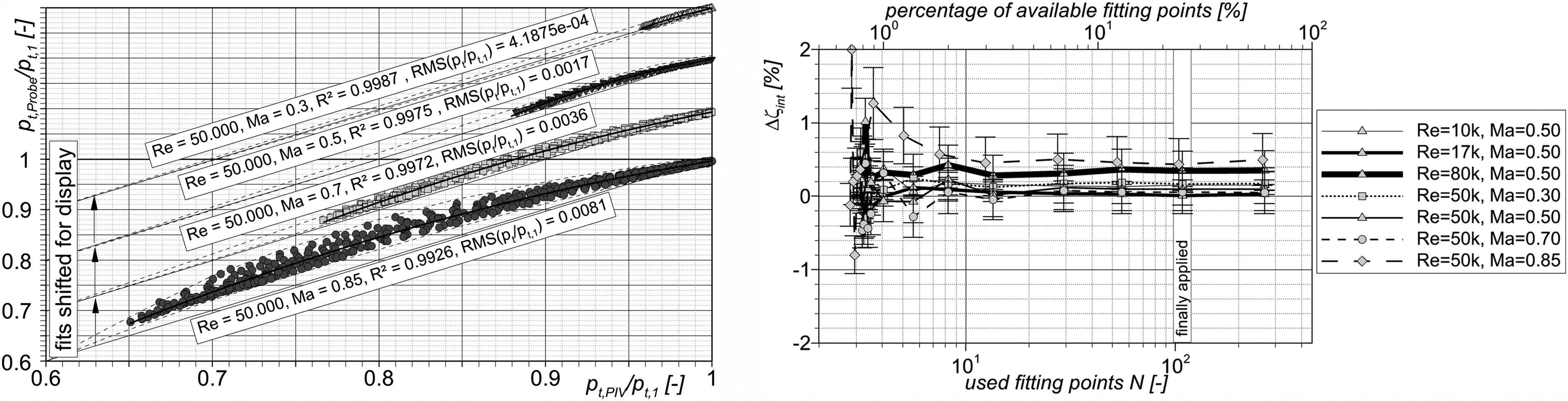
The dependency of the fit results in relation to the number of reference points
Four selected planar total pressure loss fields in the wake of the cylinder are plotted in Figure 4 representing distributions from incompressible low-Re conditions (top left) to compressible high-Re in the bottom row. The top half of each sub-figure carries the probe data and compares it to the in-situ corrected pressure data from PIV on the bottom half. The local total pressure losses
Figure 4.
Comparison between total pressure losses in the wake of a cylinder measured with pitot probe in the top half of each frame (a)–(d) and reconstructed and fitted from Particle Image Velocimetry (bottom half) at different Mach and Reynolds numbers. The traverse line plots were extracted at x / D = 10 R e D = 10,000 ; M a = 0.3 R e D = 50,000 ; M a = 0.3 R e D = 50,000 ; M a = 0.7 R e D = 80,000 ; M a = 0.7

In general, a very good local and quantitative agreement can be demonstrated. It is obvious, that the wake core close to the cylinder provides larger mismatch compared to the remaining flow field. As a consequence of strong but very thin shear gradients in this area, the pressure loss production is also significantly affected by the turbulent stresses. For a highly accurate measurement of turbulent quantities, both measurement techniques are not the perfect approach, but, at least PIV (if properly applied), can help to estimate their order of magnitude. It is also known from multi-hole probe measurements, that the geometric size of the probe head and the traversing step size may have significant impact on the measured pressure data in terms of spatial resolution, especially if the flow structures become finer and the gradients get sharper, cp. Vinnemeier et al. (1990). For this reason, conventional probe traverses for total pressure loss characterization shall be performed in the mixed-out wake, were the flow is not dominated by these sharp gradients.
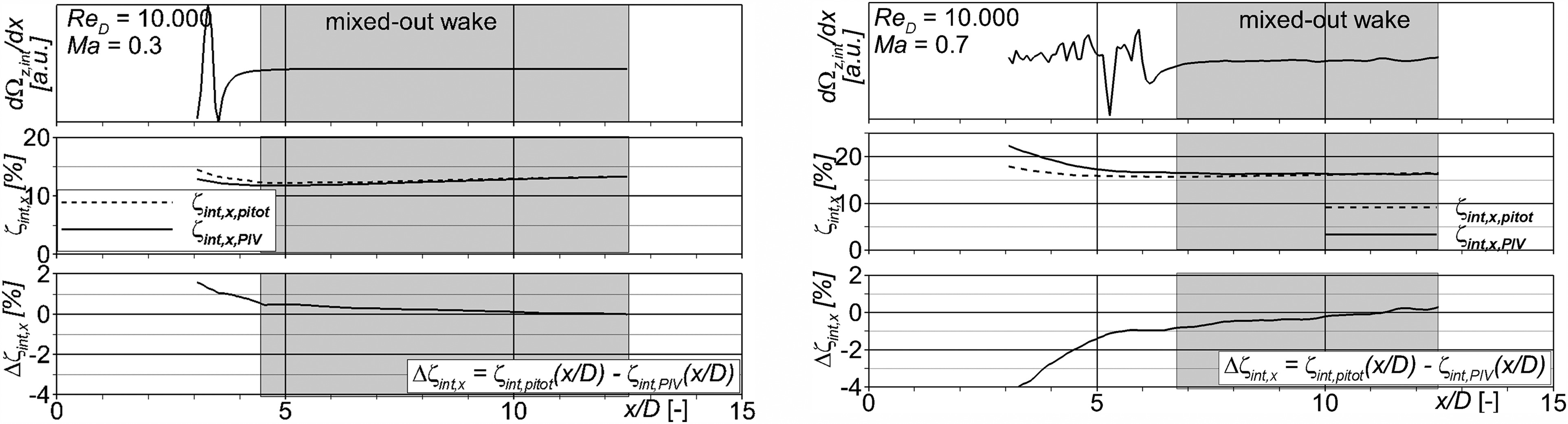
A criterion which may separate turbulent wakes between non mixed-out and mixed-out regions was proposed by Proudian (1964) who related the dominant turbulent fluctuations to the local wake velocity deficit according to
Figure 5.
Spanwise-averaged wake properties showing: the axial gradient of the “mixed-out” criterion Ω z = u ′ 2 / Δ V 2
In particular transonic (wake) flows can be of interest for the application of the proposed approach since the flow field may be complex and dominated by strong velocity and pressure gradients (shocks). By means of Figure 6, the dependency of the spatial shock position on the final interrogation window size from the PIV evaluation shall be highlighted for the operation point at
Figure 6.
Shock position as a result of a PIV grid refinement study at M a = 0.85 R e D = 50,000 d u / d x d v / d y

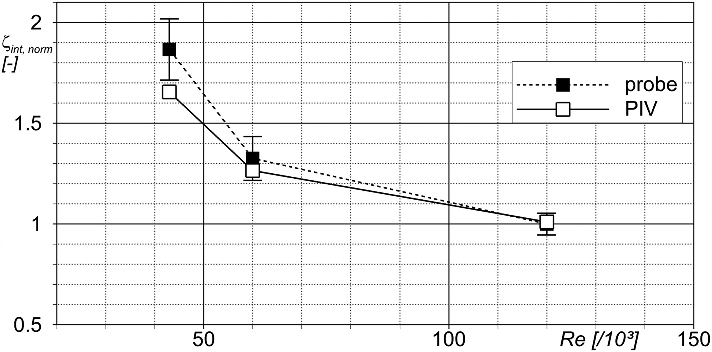
Figure 7.
Comparison of integral total pressure losses between pitot probe and PIV at x / D = 10
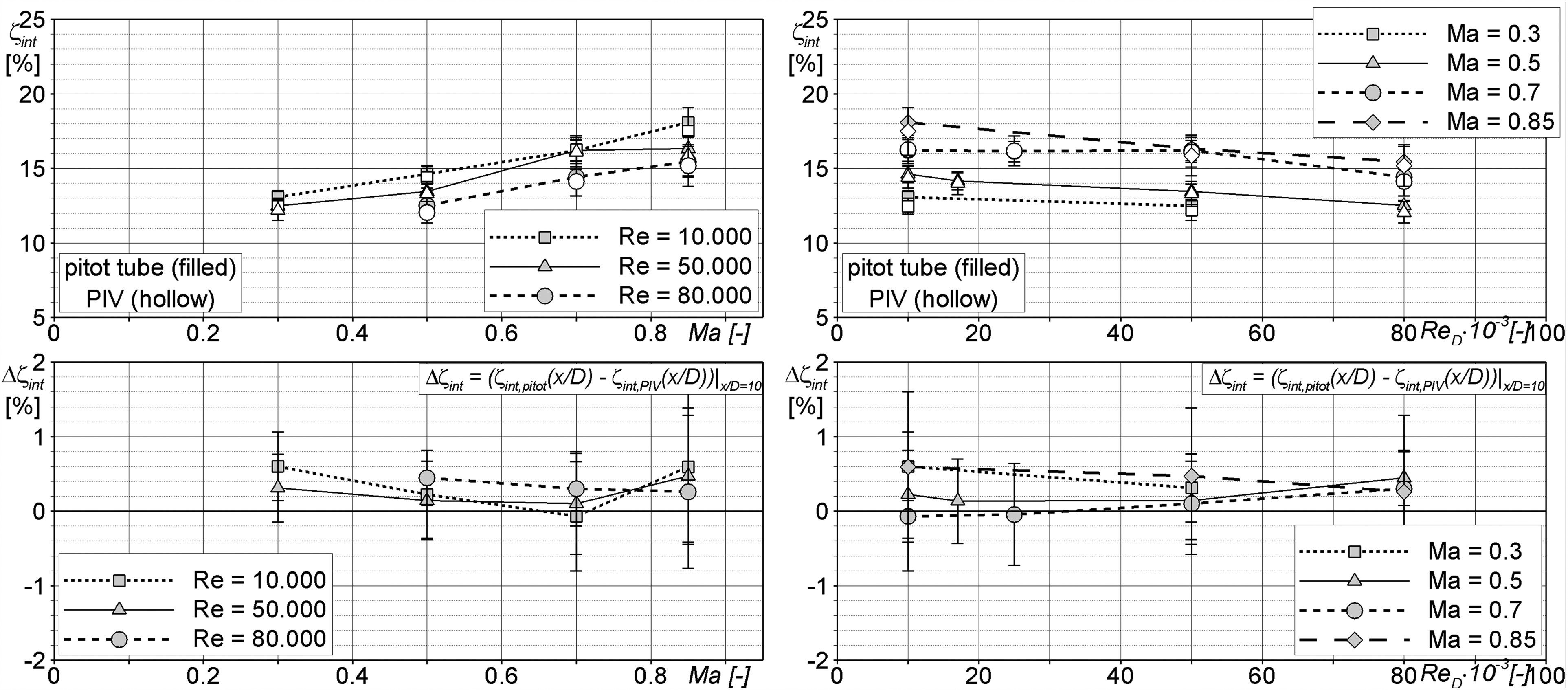
The raising trend of the integral losses with respected to the test Mach number is evident as a consequence of rising mixing losses. The negative trend of reduced total pressure losses with increased Reynolds number is also known for viscous wake flow. As a consequence of pronounced shear forces which lead to a strong shear gradient and a reduced shear layer width, the integral losses mix out more rapidly. Both trends are well prominent in wake flows, in particular for cascades flows, whose further investigation with the proposed approach is the authors’ main motivation. It is shown that both, pitot and fitted PIV pressures provide data which are in very good agreement and whose integral deviation is in the order of 1 percent or even less. The uncertainty is higher for highest Mach numbers and at lowest ambient and dynamic pressure conditions as a consequence of a) the uncertainty of the fit raises with increased Mach number as stated above, and b) the resolution of low (dynamic) pressure differences with pressure transducers of range
It can be stated in summary of all presented results so far, that the presented approach enables the reconstruction of reliable total pressure distributions from the PIV over a wide Reynolds and Mach number range when measured in the HGK facility. The relative deviations in the determination of the loss coefficient between the classic pressure measurement with a pressure probe (e.g., pitot or multi-hole probe) and the reconstructed distributions from PIV over the examined flow range are not larger than 2 % if the measurement uncertainty is considered, too. With respect to the simplicity of the presented approach, this high agreement is remarkably good, especially if the limitations (e.g. in the implementation of the pressure reconstruction scheme) are considered. It was also shown that the driving factor of growing uncertainty are increased compressibility effects due to the raised test Mach number, whereas the dependence on the Reynolds number appears to be comparatively small. With this knowledge, the approach appears to the authors to be valid enough to proof its performance at this level for a usage in cascade flows.
Low-pressure turbine cascade
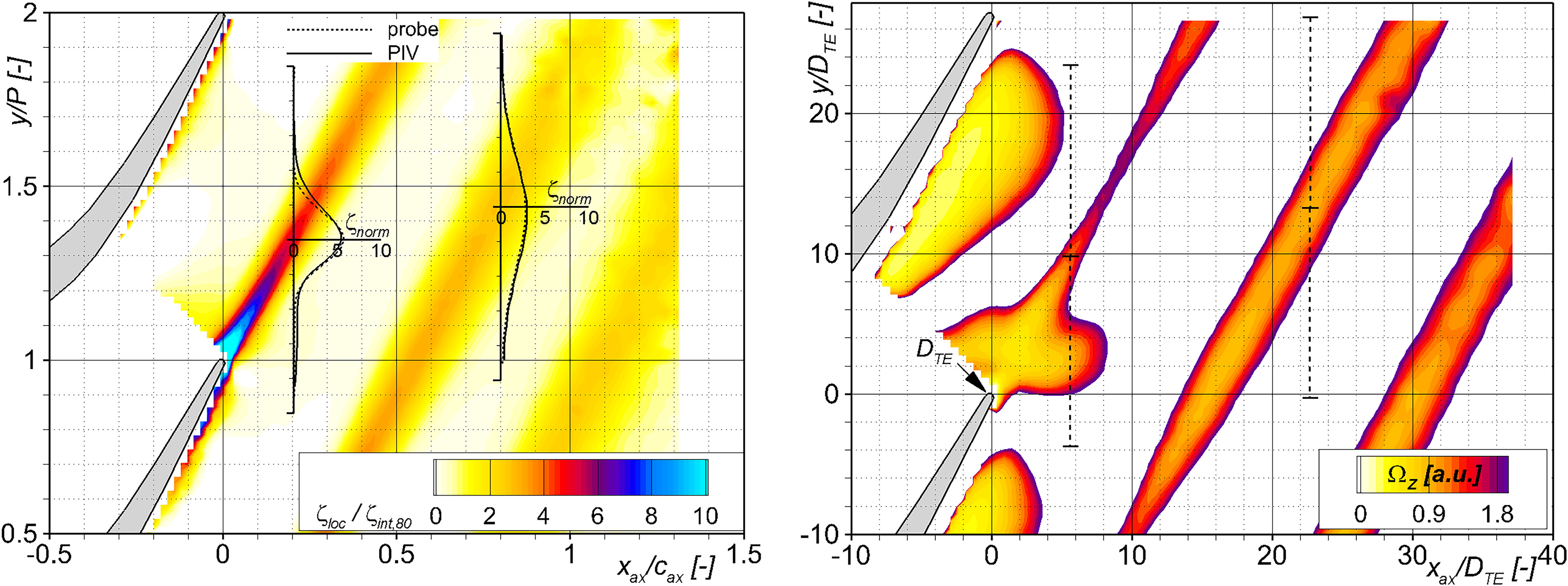
Finally, the proposed approach is applied and cross-validated to the exit flow field downstream of a low-pressure turbine (LPT) cascade comprised of 7 blades. A detailed discussion of the cascade itself and the particular flow fields at
Figure 8.
Left: Total pressure loss coefficient field in the wake of an LPT cascade at R e c = 120,000 M a e x i t > 0.6 x a x / c a x = 0.8
Conclusion and outlook
The data collected as part of this work using five-hole probe measurements and PIV enabled the development of a rather simple hybrid approach that aims to determine the total pressure distributions in wake-dominated flows as precisely as possible and with high spatial resolution. The authors’ main motivation is to expand the existing measurement portfolio with a compromise solution. This step shall combine the existing testing capabilities in a smart manner and expand the ability to provide information for the analysis of complex flow fields. The developed approach combines the authors’ many years of know-how in optical and probe-based exploration of wake flows with state-of-the-art calculation methodology for reconstructing pressure distributions from velocity field measurements as measured with PIV.
It was shown that the presented approach delivers valid results over a wide operating range, as covered by the High-Speed Cascade Wind tunnel operated at the University of the Bundeswehr in Munich for investigations of turbomachinery bladings. The investigated flow range covered a Mach number range from 0.3 to 0.85 at 3 different Reynolds numbers. The total pressure loss coefficient reconstructed from PIV, which was in-situ-corrected by means of reference points from probe-based pressure measurements, had a maximum uncertainty of approx. 2% in the entire examined operating range. In the low-speed range at
The approach presented here is based on a simple second-order polynomial fit between known reference values and the raw pressure values reconstructed from the PIV, whereby the reconstruction scheme is actually implemented for incompressible flows. In addition, the presented approach also contains isentropic assumptions when calculating the Mach number distribution from the velocity distributions of the PIV and the conversion from static pressure to total pressure. Given the combination of all these simplifications and assumptions, the relatively high level of agreement between the results is remarkably good. The users should be aware of some key factors in the flow field, which can be summarized as:
The application of the procedure seems less accurate if the measured and/or reconstructed pressure values are part of a non-mixed-out wake flow. Here, both, the pressure probe and the PIV have their own deficit and increase the accuracy of the algorithm.
The reference probes for fitting are less dependent on their actual positions but rather that they are distributed to cover values across the entire pressure range and flow field to be reconstructed. Knowing this, a fairly low number of reference probes around 20 can deliver sufficient results.
It was shown, that the application of the approach for high-speed/transonic flows is generally possible. Nevertheless, the nature of the incompressible pressure reconstruction scheme implemented in DaVis inherently limits the validity and necessitates the careful usage and questioning of the results.
Nomenclature
Latin symbols
characteristic length
cylinder diameter
test section height
Mach number
Number of data points
static; total pressure
cascade pitch
dynamic pressure
ideal gas constant
Reynolds number based on chord length or cylinder diameter
total temperature
velocity vector
axial and lateral wind tunnel coordinates
Abbreviations
5HP
five-hole probe
ax
axial dimension in blade coordinates
HGK
High-speed Cascade Wind Tunnel at the University of the Bundeswehr in Munich
IWS
Interrogation window size
exit
exit condition
LPT
Low-Pressure Turbine
norm
normalized value
PIV
Particle Image Velocimetry
ref
reference condition
RMS
root-mean-square value