
Introduction
Turbomachinery test facilities range from simplified-geometry test tunnels for initial concept testing and fundamental research (at the low technology readiness level (TRL) end of the scale), to full-scale engine test-beds for product demonstration (very high TRL). Between these extremes, there are a small number of high-TRL test facilities that replicate the engine environment with high fidelity (sometimes using engine parts, and with good dimensional scaling) but which offer advantages over full-engine testing.
One such facility is the Engine Component AeroThermal (ECAT) facility at the University of Oxford. The facility is used for high TRL research and development, new technology demonstration and for component validation. The facility uses a full annulus of engine parts (typically HP NGVs) achieves high similarity to engine conditions, matching Reynolds number, Mach number and coolant to mainstream pressure ratio. A combustor simulator module is also available for combustor-turbine interaction studies with rich and lean burn temperature, swirl and turbulence profiles. The facility has lower operational costs than typical engine test beds (at least order-of-magnitude cost reduction) but the prime advantage lies in the accuracy of measurement: the facility was designed to reduce uncertainty in a number of key measurements to a minimum.
The ECAT facility operates in blow-down mode from high pressure air receivers. The mainstream flow for the current warm-cores (modular design) for the facility is heated with two 1 MW electric air heaters. For a HP NGV ring from a large civil engine operating at cruise conditions of Reynolds and Mach number, the maximum achievable coolant-to-mainstream temperature ratio is 1.28. The ECAT facility is described in detail by (Kirollos et al, 2017).
This paper describes a major upgrade to the ECAT facility, which will allow engine-realistic coolant-to-mainstream temperature ratios to be reached. The two significant aspects of the upgrade are the infrastructure for a hot air system, and a hot-core for the ECAT facility test-bed. When the upgrade is complete, all important non-dimensional parameters will be matched to engine conditions, providing a test vehicle which is very close in its capability (so far as HP NGVs are concerned) to a thermal-paint-test engine.
To predict and optimise the operating characteristics of the hot-core, a low order transient thermal model was developed. This was validated using experimental data from the ECAT facility warm-core. Results from the low-order model informed architectural decisions for the hot-core design. In particular, decisions regarding: impact of trace-heating on tank and feed-pipe system; sizing of the feed-system pipework (including mass-metering nozzles, flow regulators etc.,) to achieve the operational range of the facility; the burst-relief analysis; run-time analysis at different operating points; simulations of metal effectiveness characteristics. Results from the model, including the validation data, are discussed in detail in this paper.
The mechanical design of the working section is also discussed, the major challenge being that of the rapid heating of the working section components and the consequent high transient thermal stress. The design was initially optimised by extending the transient thermal model to calculate component stresses arising from transient thermal loads internal pressure, before more detailed calculations using a transient finite element code (Ansys Mechanical) were carried out. Measurement from the warm-core ECAT facility have been used to provide heat transfer boundary conditions.
The ECAT facility warm-core was developed from earlier facilities already at a high level of maturity, e.g. (Luque and Povey, 2011; Povey et al, 2011; Kirollos and Povey, 2017). Unusually for an ambitious facility build, both the ECAT facility test-bed, the warm-core, and a number of associated research programmes were delivered on time and within budget. This was the result of an incremental development process (bringing together existing components which were individually well understood), with thorough prediction of all aspect of facility performance during the preliminary design phase. This approach extended from analysis of the air system, all the way through to understanding and optimising the measurement uncertainty of all underlying measurements required for metal effectiveness, capacity and aerodynamic traverse measurements. In our experience (having developed a number of similar facilities, and having advised on the development of many more), this level of analysis during the preliminary design phase is unusual, and we hope can form an example of some of the ways (this paper is not exhaustive by any means) in which good practice can be achieved at an early stage in major facility development projects.
Scaling of heat transfer parameters
Typically in the warm-core ECAT facility close to cruise Reynolds number can be achieved venting directly to atmosphere and max take off (MTO) Reynolds number matched with outlet pressure control. However with increased mainstream temperature outlet pressure control is required to meet both cruise and MTO conditions.
Temperature has a significant effect on a number of variables, including conductivity (mainstream, coolant, metal), isobaric specific heat capacity (mainstream, coolant), ratio of specific heat capacity, and viscosity. These parameters are summarised for engine cruise, warm-core and hot-core ECAT temperatures in Table 1. Reynolds number, Mach number, coolant the mainstream pressure ratio (p0c/p0m), and geometry are all matched between tests.
Table 1.
Comparison of warm-core, hot-core and cruise engine conditions properties.
| Engine | Hot-core | Warm-core | ||
|---|---|---|---|---|
| T0m | K | 1500a | 600 | 350 |
| T0c | K | 800 | 280 | 280 |
| Reb | 3.05 × 10⁶ | 3.05 × 10⁶ | 3.05 × 10⁶ | |
| M | 0.95 | 0.95 | 0.95 | |
| kNGV | W/mK | 25 | 12 | 10 |
| kfluid | W/mK | 0.1000 | 0.0456 | 0.0297 |
| Bi | 0.40 | 0.38 | 0.30 | |
| cp1 | J/kgK | 1276 | 1051 | 1008 |
| cp2 | J/kgK | 1099 | 1004 | 1004 |
| cp1/cp2 | 1.161 | 1.047 | 1.004 | |
| γ | 1.29 | 1.38 | 1.40 | |
| μm | m2/s | 5.30 × 10⁻⁵ | 3.03 × 10⁻⁵ | 2.08 × 10⁻⁵ |
The temperature will also have a small, although significant effect on the capacity of the NGVs due to component thermal expansion, and which is corrected when comparing cold capacity measurements taken in the warm-core ECAT facility to engine conditions (Povey et al., 2011). These effects, whilst important for the engine designer, are small enough to be excluded from the design calculations described in this paper.
Facility architecture
The facility is a transient facility that maintains engine representative conditions for a reasonably short duration (typically 40–50 s depending on the test conditions in the high temperature facility). Air receivers (tanks) will be gradually pressurised and heated to 50 bar (gauge) and 600 K. The air is released to the working section, housing the engine components under test. A facility of this nature has advantages over a continuously operating facility, principally the lower cost of operation compared to a continuous facility through reduced energy requirements and simpler hardware whilst still providing the same test objectives except endurance testing.
Air supply and metering
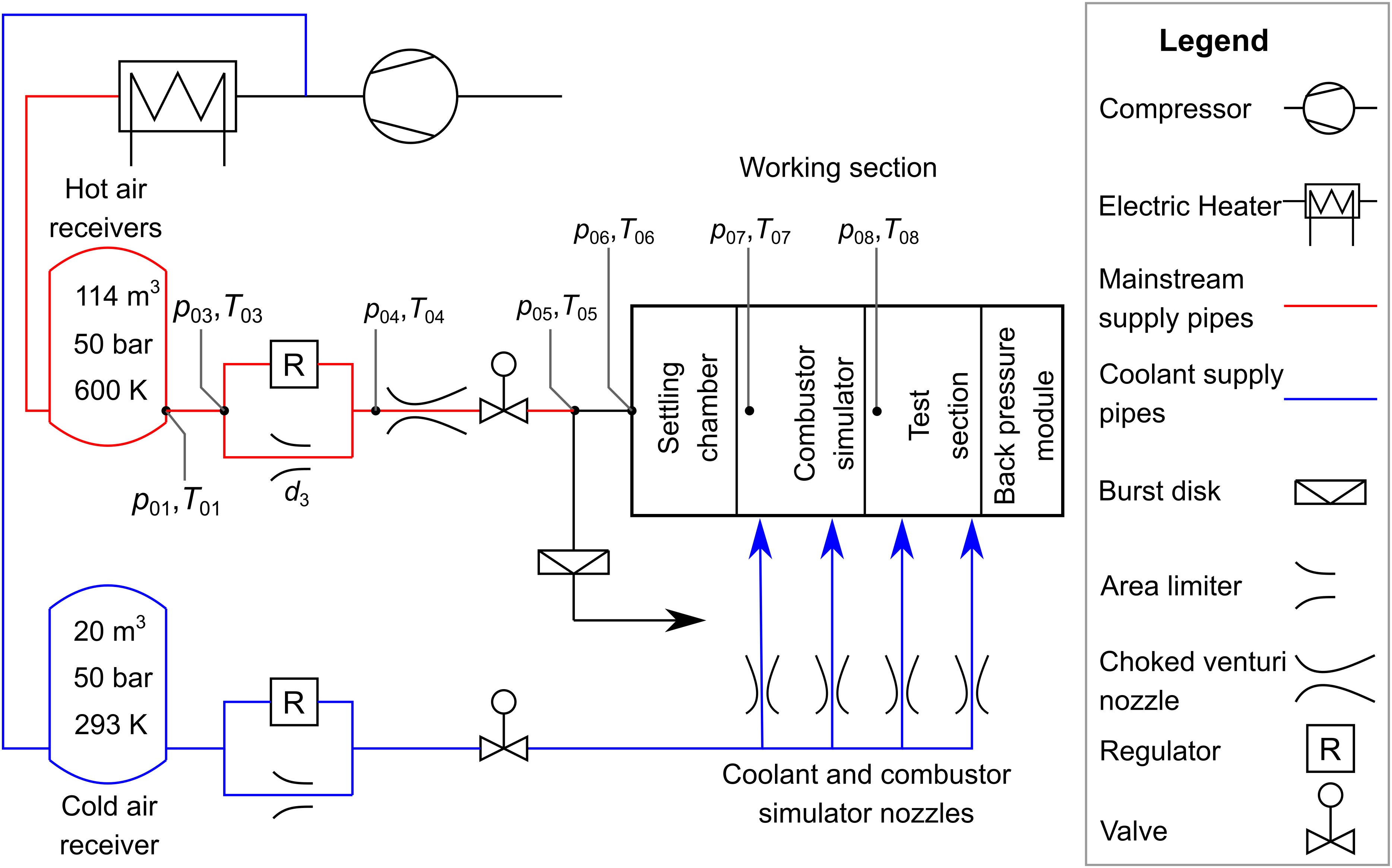
Air to the test facility will be supplied from 3 × 38 m3 heated and insulated air receivers for the mainstream flow and a single 20 m3 air receiver at ambient conditions which supplies coolant air to the components under test. The previous warm-core iteration of the facility used two 1 MW electric air heaters to heat the mainstream flow to a modest level. In the upgraded facility the mainstream inlet temperature (T0m) is controlled by setting the temperature in the tanks (T01).
The air flowed through a pressure regulator and limiting nozzle before flowing through a choked venturi nozzle, built to ISO 9300 and calibrated at Colorado Engineering Experiment Station Inc. (CEESI). The nozzle allows very accurate (<0.25%) measurement of the mainstream flow through the working section. Coolant and the supply for the combustor simulator (OTDF) module was metred separately with individual choked venturi nozzles also manufactured to ISO 9300. A schematic layout of the facility air supply system is shown in Figure 1. There is an unheated section of pipe in front of the working section to enable the working section to be worked on while the upstream pipework is heated by the trace heating system.
Working section
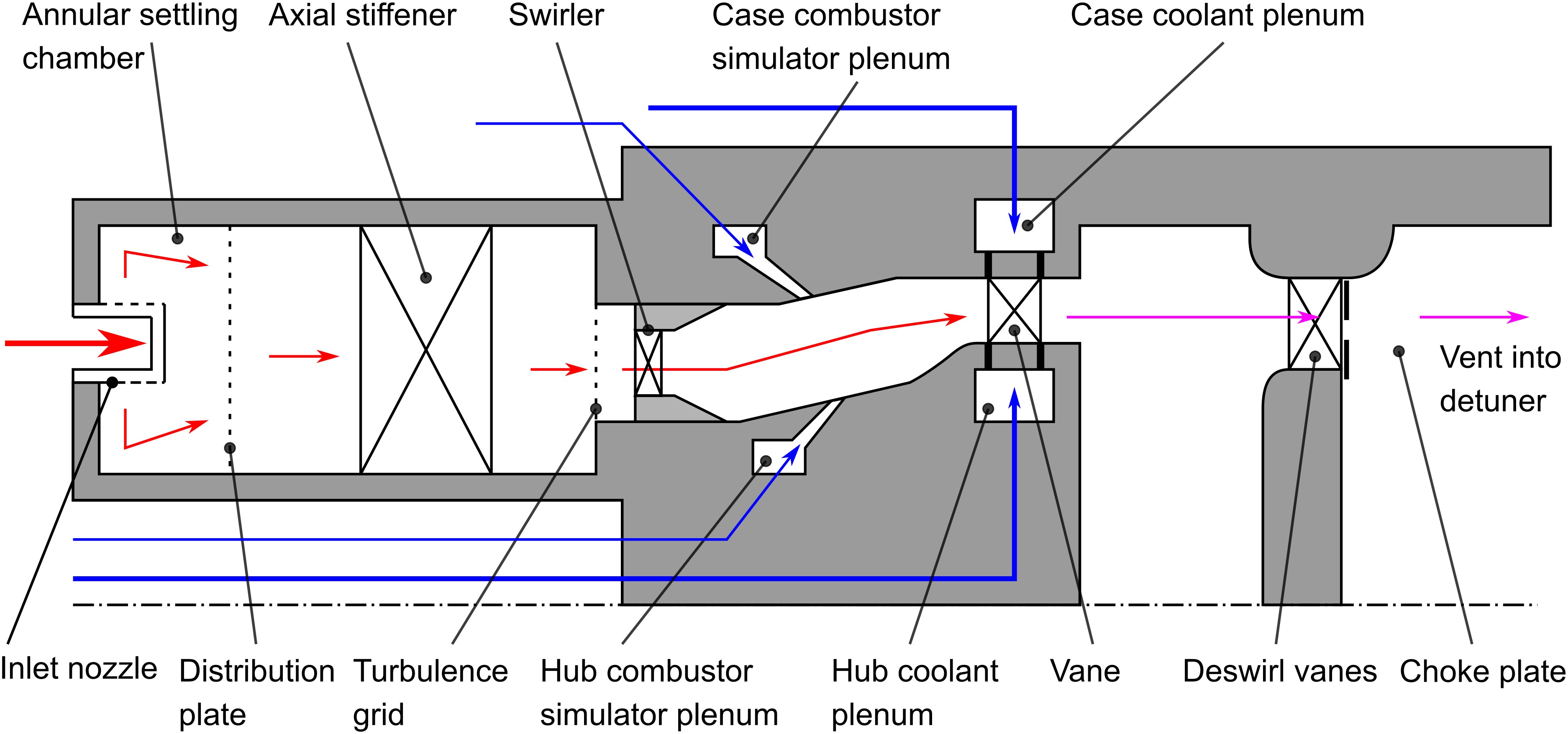
The working section comprises a number of separate modular sections, shown in Figure 2. The first module is a settling chamber which conditions the flow, followed by the axial stiffener which transmits the axial load from the hub to the case. There is then the combustor simulator module, followed by the engine components under test. The rear module includes a set of de-swirl vanes and a choke plate to set the pressure downstream of the test components before the flow is vented into the silencer. It is possible to operate the facility without the combustor simulator and/or the choke plate assembly depending on the desired test conditions. A burst disk positioned in the upstream pipework protects the working section from over pressure.
The working section will be instrumented with pressure and temperature rakes and surface measurements. These include component surface temperatures, mainstream temperature profile, surface pressure and mainstream pressure profile. In addition, infra-red thermography will be used (methodology described by Kirollos et al., 2017), upstream and downstream of the vanes.
Because of the high temperature and pressure of the facility, bespoke pressure-rated and cooled camera modules have been developed. The working section will also be equipped with a traverse system downstream of the test components. This is a second-generation design based on the system successfully deployed in the warm-core for ECAT. Together the range of instrumentation allows heat transfer measurement (such as overall metal effectiveness) and detailed aerodynamic loss measurements to be taken.
Facility transient thermal and flow model
Because of the semi-transient (time constants which are long compared to thermal/flow stability of the test part, but short so far as thermal soaking of the core is concerned) operating principle of the facility, unsteady thermal loads are significant in determining the time variation of the feed temperatures to the facility during a run. The mainstream temperature history—in particular—is a function of the pre-run tank condition (pressure and temperature), and the temperature history of the feed system and working section. The latter depends significantly on the run history (number of runs and dwell time between each run) prior to a particular test, and to a lesser degree on the time history ambient conditions in the test area.
To predict these complex interactions, a transient thermal model was developed in Matlab. This calculates the temperature of the mainstream and coolant flows during a test run, taking account of: isentropic expansion in the main tanks; heat transfer in all elements of the feed system and tank system; trace heating systems; and loss to the environment through lagged and unlagged elements of the facility. The model has been carefully validated against existing data from the warm-core facility.
We now describe the overall structure of the facility (situation to be solved), the general solver structure and method of solution, calibration against existing data, and final predictions of the operating point of the ECAT hot-core.
Structure of the transient thermal model
The facility delivery pipework and working section are modelled as a series of distributed thermal masses, as shown in Figure 3. Heat is passed between the fluid and the pipe or working sections walls by convection. The latter are discretised radially, to ensure accurate modelling of the thermal time constants of different components. Heat exchange with the external environment (natural convection and radiation) is also modelled. Most of the heat exchange (between fluid and solid) occurs in components with extremely high thermal aspect ratio (very thin walls in comparison to overall pipe length). We therefore only consider radial conduction, and accordingly describe the solver as “1.5 D”.
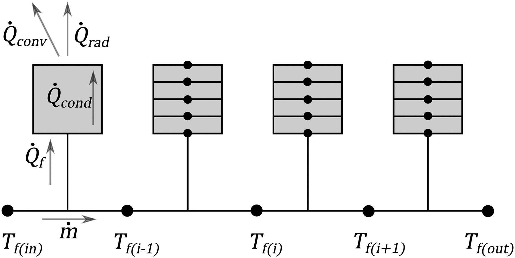
An explicit scheme was used to calculate the transient radial conduction in each block (see, e.g. (White, 1988)), using time marching with a suitably small time step to ensure convergence stability. The time step depends on the size of the radial discretisation, the metal conductivity and the convective heat transfer coefficient at the boundary. All the thermal masses are axisymmetric in nature, and therefore the change in radial area of each element has been accounted for.
To ensure a physically reasonable form for the variation with flow condition of the internal Nusselt number, a modified version of the Dittus-Boelter correlation (smooth wall turbulent pipe flow) was used in the model:
where—importantly—NP is a tuned parameter, which was adjusted using calibration data from the facility. Following a similar process, a second tuned parameter, NWS, was used in the working section model.
For the external heat transfer coefficient, the horizontal cylinder correlation of (Churchill and Chu, 1975) was used:
where for the working section (which has irregular geometry), the tuning parameter Nex was determined using warm-core experimental data.
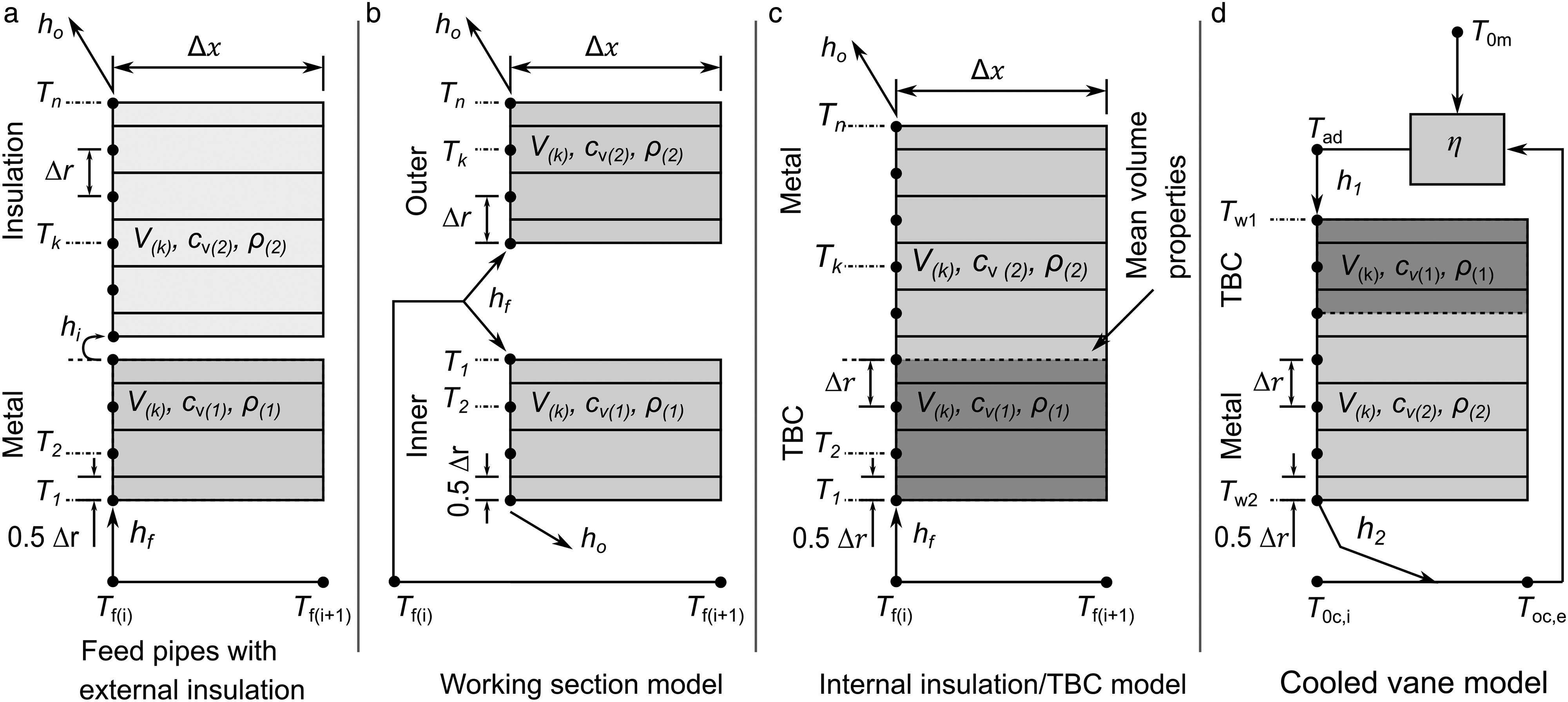
The prime purpose of the model was to inform key design decisions for the hot-core of the ECAT facility. The model allows detailed analysis of the impact on run conditions of, for example, external insulation on the pipework, and internal low conductive liners (for example TBC applied on the inner walls of the pipe and working section). In addition, the impact of typical running cycles (number of runs and dwell time between each) on test conditions can be established. To do this, the model was run with a number of different distributed mass models. Four archetypal models (used variously as blocks within an overall facility model) are shown in Figure 4, illustrating: (a) pipes with external insulation; (b) working section model with external insulation; (c) working section with internal insulation (e.g. TBC); (d) cooled nozzle guide vane to determine the vane transient response under various operating conditions.
Pipes with external insulation
The model for pipes with external insulation is shown in Figure 4a. Axisymmetric elements are discretised in the radial direction, allowing for a wall block (metal), an air gap modelled with a heat transfer coefficient assume to be 50 W/m2K (if required), and an outer insulation block. Due to the high thermal resistance of the insulation, the model is insensitive to the air gap heat transfer coefficient. The model has a representation of a heat source in the gap between insulation and pipe metal to simulate the effect of trace heating of the pipes.
Working section model with external or internal insulation
Two working section models are shown in Figure 4b and 4c. In a similar manner to the pipe model, there is a representation of insulation on either the outside (Figure 4b) or inside (Figure 4c) of the working section. These two design extremes were investigated to understand the impact of these designs possibilities on three issues of concern during the preliminary design phase: (i) the stability of the transient inlet temperature characteristic of the facility, which for the hot stream becomes generally more stable with the addition of external insulation and/or pre-heating, but which for the cold stream behaves in the reverse manner; (ii) the thermal stresses imparted to the working sections parts during the semi transient run, which in general decrease with internal insulation (lower heat flux on account of thermal barrier) and pre-heating (lower heat flux on account of lower temperature difference); (iii) the peak temperature of the working section components over a typical daily duty, which increase with external insulation (less heat loss) and decrease with internal insulation (less heat transferred from the fluid).
These issues are discussed in detail in subsequent sections. We will see that it is necessary to maintain the feed pipes at temperature in-between runs (using trace heating and lagging) to sufficiently stabilise the transient inlet temperature characteristic of the facility, but that—in contrast—reducing heat transfer to the working section with a layer of internal insulation, and allowing natural cooling of the facility between runs (no external insulation), has the advantages of reducing the peak temperature of the outside of working section during test campaigns, reducing thermally-induced stress during the semi-transient operation, and has relatively minimal adverse impact on the inlet temperature transient.
Cooled vane model
The cooled vane model is shown in Figure 4d. This is the same as that used by (Kirollos and Povey, 2016). The ECAT facility typically operates with either real engine hardware (HP nozzle guide vanes) or engine-scale laser sintered hardware. The non-dimensional boundary conditions for the model were based on generic engine conditions reported by (Kirollos and Povey, 2016). The dimensional boundary conditions of the model (for example the external and internal heat transfer coefficients) were scaled to the conditions of the hot-core ECAT facility, as was the vane thermal conductivity. The impact of an external layer of TBC was also considered during the modelling. Heating of the coolant inside the vane is calculated as per Equation 3, and the mean film temperature (Tad) on the external surface of the vane is calculated as per Equation 4, assuming an adiabatic film cooling effectiveness (η) of 0.5.
Thermal model of the air receivers
The discharge of the air receivers (tanks) has been modelled by applying the unsteady energy equation to the volume of air inside the air receiver, Equation 5 (see, for example, (Rogers and Mayhew, 1992)).
δm(j) is the mass of air removed in a particular time step j, m the mass of air in the tank at a particular time step, and Q the heat energy transferred from the tank walls to the fluid in a particular time interval. The tank metal is treated as a single lumped thermal mass (Bi = 0.0625) with variable metal temperature, and with no heat transfer to or from the environment (the tanks will be well insulated on the external surface). The heat transfer from the internal wall of the tank to the enclosed air was modelled assuming a modified Rayleigh number correlation for free convection in an enclosure:
where NT is a tuned parameter adjusted to match data from the warm-core facility. The Rayleigh number is defined as:
where D is the tank diameter; Tw and Tf the tank wall temperature and air temperature respectively; and g, α and ν the acceleration due to gravity, thermal expansion coefficient (of the internal fluid) and kinematic viscosity respectively.
Mass flow rate models for the facility
Two mass flow models of the facility have been developed. A steady state pressure model coupled with the transient heat transfer model to simulate a full test run (typically 80 s or longer), and an adiabatic transient pressure model to simulate instantaneous pressures during start-up (typically first 10 s). These models are now discussed in turn.
Steady state mass flow rate model
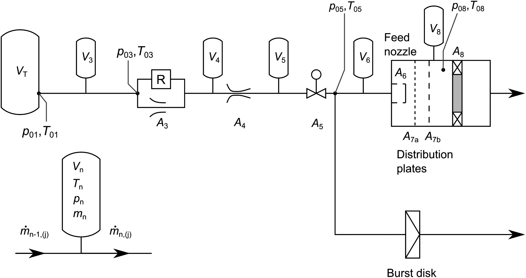
The facility flow rate can be thought of as being controlled by the pressure loss through a network of restrictions, shown in Figure 5, with the boundary conditions of an upstream total pressure (decaying tank pressure) and an atmospheric backpressure. There are three restrictions of particular note: the (variable area) regulator and adjustable limiter system upstream of the main critical venturi nozzle (A3); the main critical venturi nozzle (A4); and the HP nozzle guide vane ring (A8). Depending on the instantaneous running condition, it is possible for all three of these significant limiting areas to be independently choked (at—generally—very different total pressures, but similar temperatures), or, at the other extreme, for none to be choked. The flow through the network is calculated using (locally) isentropic compressible flow equations. The facility operates in two distinct modes: blowdown mode and regulated mode. We consider each of these in turn.
Figure 5.
Schematic diagram of the steady state and transient flow models. Filling of the pipe volumes (V3 to V8) is only considered in the transient pressure model.
In blowdown mode, the tank is charged to pre-run conditions of temperature and pressure, the isolation valves fully opened, and the tank allowed depressurize naturally. This mode of operation is used, for example, to determine capacity characteristics.
In regulated mode, a bypass regulator arrangement (regulator plus area limiter system) maintains a constant pressure upstream of the venturi nozzle, delivering approximately (slowly reducing total temperature) constant mass flow rate to the nozzle guide vanes under test. The limiter is sized to achieve the correct mass flow rate at start-up (maximum tank pressure). The regulator (an 8″ Oxford Flow IHF regulator) size determines both the run length, and the consequences under equipment failure (e.g. regulator fully opens), which in turns determines the burst relief requirements for the facility. The optimum design of this facility led to a test duration of 65 s.
Transient mass flow rate model
A transient version of the mass flow rate model was developed to understand the filling and emptying characteristics of the pipe volumes between restrictions. The primary use of this model was to determine the fastest valve opening times. Fast valve opening times create pressure transients which risk rupturing the burst disk.
The transient flow model uses the same network of restrictions as the steady-state model, but the volumes between restrictions are additionally modelled. This is shown schematically in Figure 5. Pipe volumes are associated with each section between the limiting areas. The temperature in the pipe volumes is governed by the change in mass (of air) in the volume, and conservation of energy for each pipe volume. The kinetic energy of the fluid entering and leaving the volume is neglected, as is heat transfer with the pipe wall. This approximation is justified by the fact that the pressure time constant of the flow is much smaller than the thermal time constant of the pipe wall. The incoming and outgoing mass flow rates (and therefore the mass of fluid in the volume at each time step) are found using the same equations as for the steady state flow model. In the transient model, the instantaneous pipe volume pressures determine the upstream and downstream boundary conditions. Once the masses of fluid contained in each volume are determined, the pressures at each time step are found from the equation of state for a perfect gas. The nomenclature for an isolated pipe volume is also shown in Figure 5.
Comparison of low-order and high-order models and calibration against experimental data
We now compare our low-order model to an Ansys Mechanical transient thermal analysis and lumped mass model, and then we calibrate the model using experimental data from the warm-core ECAT facility. The calibrated model is then used to predict the operating point of the new facility.
Comparison of low-order and high-order models
A comparison was made to a transient thermal simulation conducted in Ansys Mechanical. The geometry modelled was a 100 mm long section of 8 inch Schedule 40 pipe (219.1 mm OD; 202.7 mm ID). The Ansys Mechanical model had 20 radial elements. The starting temperature was 293 K and the fluid temperature was 600 K, with a heat transfer coefficient applied on the internal surface, and all other surfaces were perfectly insulated. The same conditions were replicated in the Matlab model. Automatic time step sizing was used with a minimum time step size of 0.1 s, initial time step of 0.1 s and the maximum 4 s. The models were run for 80 s. The Matlab model radial discretisation was varied, ranging from 5 radial elements to 20 radial elements, as summarised in Table 2. The time step size was chosen to be approximately the largest step size to maintain stability. The surface temperature transient is shown in Figure 6 and shows close agreement between the two models with 10 radial elements or more (or 5 radial elements and a reduced time step).
Table 2.
Number of radial elements and time step size used in the model verification.
| No. radial elements | Time step (s) | |
|---|---|---|
| n5a | 5 | 0.080 |
| n5b | 5 | 0.005 |
| n10 | 10 | 0.020 |
| n20 | 20 | 0.005 |
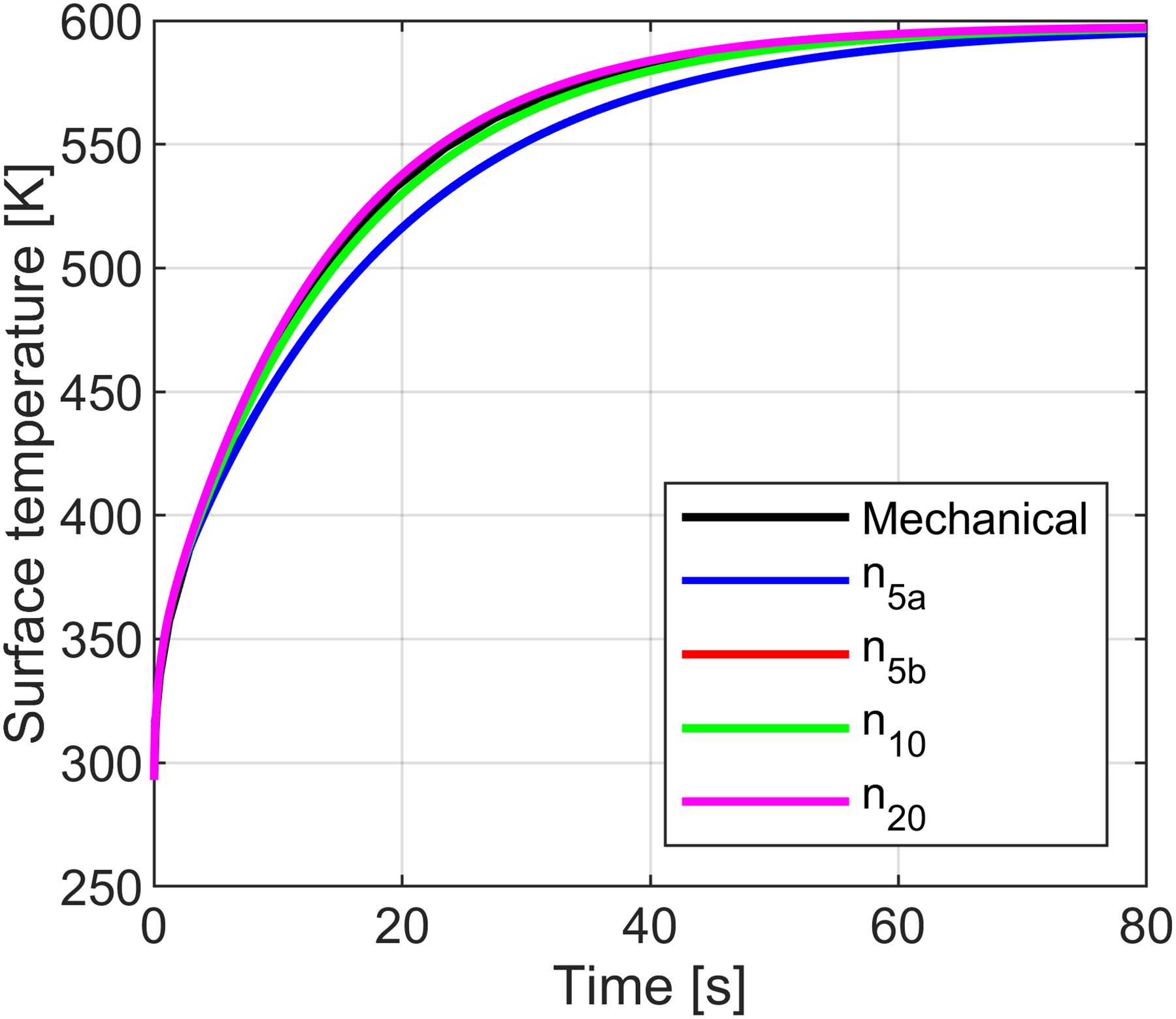
For all levels of radial discretisation the models show the same steady state temperature. This was taken to be a cross-check of the basic mechanics of the low-order solver.
Model calibration using experimental data
The model was calibrated using data taken from the existing ECAT facility warm-core, to determine the value of a free coefficient (associated with the absolute scaling of the heat transfer coefficient, but not the form of the function with Reynolds number) for both the pipe sections and the working section.
The pipe model, tank model and working section model were calibrated separately. The measured temperature upstream of the nozzle, T04 (see Figure 1), was used as the input to the pipe model and the coefficient NP adjusted until agreement between the model output and the measured temperature at the input to the working section (and a significant distance downstream of the nozzle), T05, was reached. This is shown in Figure 7, and which shows good agreement between the measured temperature, T05, and the output temperature from the tuned model, T05 (mod). Note that here we are primarily concerned with the form of the trend, which is well matched across the duration of the run. Experimental data from a test at the beginning of the day was used so that the initial facility pipework temperature was relatively uniform.
Figure 7.
Calibration of the pipe and tank transient thermal models using warm-core ECAT facility data.
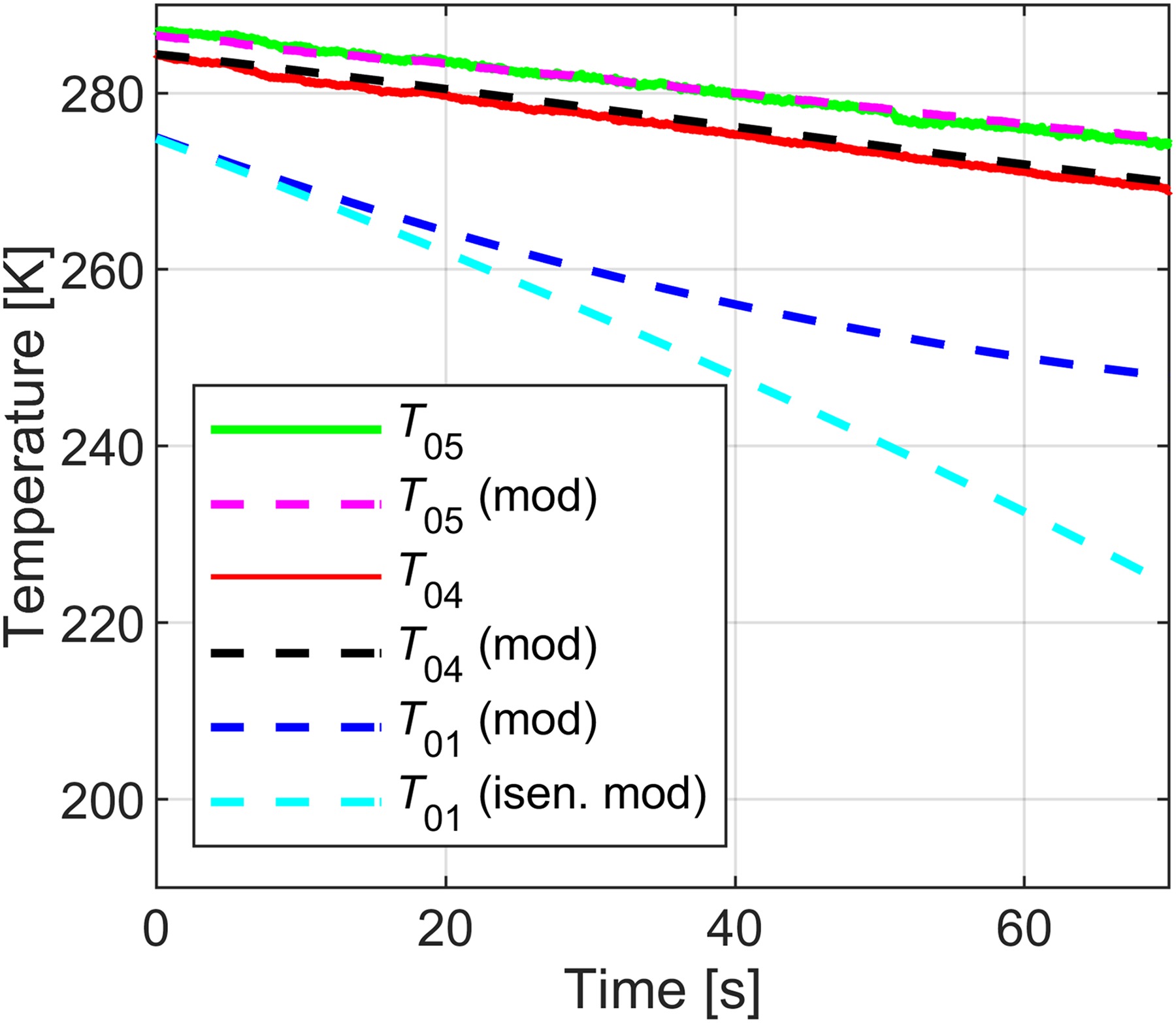
There are no thermocouples installed in the air receivers of the warm-core ECAT facility, so to evaluate the tank tuned parameter, NT, the calibrated pipe model was run (with tuned coefficient NP taken from the previous step) between the tank exit (station 1) and the nozzle inlet (station 4), and NT adjusted to achieve the best match between the measured and modelled temperatures at nozzle inlet (T04 and T04 (mod)). This comparison is shown in Figure 7. An excellent match between the trends is achieved.
The modelled tank temperature, T01 (mod), and the tank temperature assuming purely isentropic expansion, T01 (isen. mod), are also shown in Figure 7. The strong divergence between these trends shows the importance of using a heat transfer model for the estimation of tank outlet temperature. For completeness, we note that the air receivers and some pipework elements are located outside the building, hence have a different initial temperature, which must be accounted for in the modelling (depending on the daily temperature).
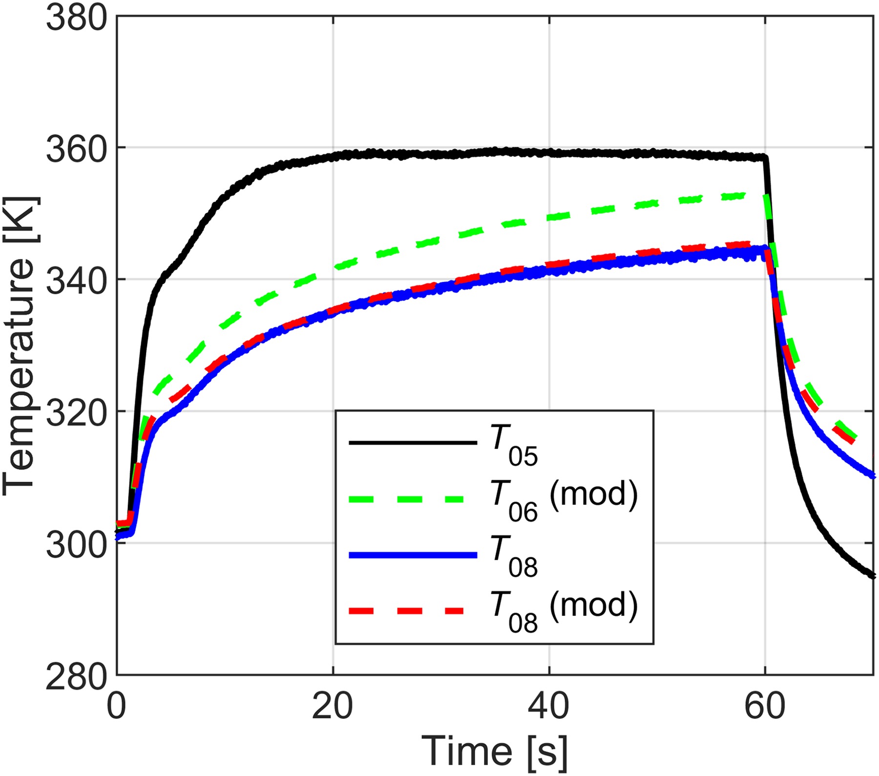
The working section thermal model was calibrated in a similar manner to the pipe model. The procedure was as follows. The facility inlet, station 6 (see Figure 1), was not instrumented in the warm-core facility, and is separated by a significant length of pipe from station 5. Thus T06 can be related to T05 using the tuned pipework model. This was run to predict T06 (mod) from measured data at T05. This comparison is shown in Figure 8. Using the working section inlet temperature, T06 (mod), the working section tuned parameter was then adjusted to give agreement with the modelled and measured temperatures at the outlet of the working section, or NGV inlet plane, station 8. The comparison between these temperatures, T08 and T08 (mod), is shown in Figure 8. Excellent agreement between the measured and modelled temperatures is achieved, justifying the importance of the experimentally tuned model.
Figure 8.
Calibration of the working section transient thermal model using warm-core ECAT facility data.
The working section natural convection cooling model was tuned using data from thermocouples mounted on the outer surface of the working section. A comparison between the modelled (Equation 2) and measured temperature decay is shown in Figure 9. For completeness, a summary of the tuned parameters is given in Table 3.

Model results and conclusions
We now use the calibrated analytical transient aero-thermal model to predict the performance of the ECAT facility hot-core, for various plant configurations (e.g. pipework layouts and sonic meter sizes) and thermal treatments (e.g. internal TBC and external lagging). The results from this modelling exercise informed key design decisions, which are elaborated in the following section. In particular, we consider: the optimum mainstream (choked venturi) nozzle size; optimum pressure regulator size; the necessity (or otherwise) for air feed system pipework heating; and the effect on the precise operating point of multiple daily tests. The test components are NGVs from a large civil turbofan engine, to be operated at cruise conditions of Mach number, Reynolds number, and coolant-to-mainstream temperature ratio.
Sizing of nozzle and regulator
The mainstream choked venturi nozzle and regulator were sized to balance the conflicting requirements of maximising the run time, whilst allowing for reasonable safety case scenarios related to discharging the feed mass flow rate though a burst relief system in the event of overpressure (caused by failure-induced blockage in the working section). The temperature stability of the facility during the run period was also considered as part of this analysis.
Figure 10a shows a comparison of the predicted run time for 3.25″ and 3.50″ (throat) diameter nozzles with 6 or 8 inch nominal diameter regulators (Oxford Flow regulators are to be used because of their high-temperature capability; as used in the warm-core ECAT). The tank pressure is shown, and p04, which is the pressure upstream of the nozzle. The vertical dashed lines indicate the test duration, which ends when the required mass flow rate can no longer be supplied by a fully open regulator. Initially the regulator is closed and the mass flow rate set by the size of the limiter (of equivalent diameter d3 in Figure 1), which has been sized to pass slightly more mass flow than the nominal condition in the first 5–7 s of the run while the test facility conditions stabilise (where no useful data would be obtained). This puts the test facility on condition for the full range of the regulator stroke.
Figure 10.
Effect of mainstream nozzle size and regulator: (a) Effect of mainstream nozzle size on regulator set pressure and run time. Vertical dashed lines indicate the test run time; (b) Mass flow rates for the safety cases of the regulator failing fully open for combinations of two nozzle sizes (3.25″ and 3.50″) and two regulator sizes (6″ and 8″) for cold inlet flow (worst case scenario). The outlet mass flow rates at 15 bar abs. and 600 K (the worst-case scenario at the maximum rated pressure) are shown for both 8″ and 12″ burst disks.

Increasing the size of the main-flow metering nozzle increases the theoretical maximum run time as the required flow rate can be passed at a lower nozzle inlet pressure, allowing for operation at lower tank pressures. To achieve close to the maximum theoretical run time, the overall size of the regulator and bypass limiter, as well as the fraction of the combined area that is made up by the fully open regulator at the limiting condition are both increased when moving in this direction, however, leading to increased regulator cost. The safety case is also more challenging to deal with, due to higher mass flow rates if the regulator fails fully-open at the beginning of the run.
The safety cases are considered in Figure 10b, in which the mass flow rates under regulator failure (failed fully open) conditions are given for combinations of two nozzle sizes (3.25″ and 3.50″) and two regulator sizes (6″ and 8″). The following hypothetical worst case failure conditions are taken: 280 K inlet temperature to the nozzle and bypass regulator system; 600 K outlet temperature from the burst relief system at the working section. The first of these boundary conditions is worst-case because cold inlet flow maximizes the inlet mass flow rate to the system. The second boundary condition is worst-case because maximum temperature ratio between the working section (outlet) and the limiter/regulator (inlet) maximises the capacity ratio requirement between the burst relief system and the (combined) limiter and bypass regulator: for a fixed tank pressure (50 bar) and working section design pressure (15 bar abs.) the capacity ratio requirement scales as
Based on this analysis, it was concluded that a 3.50″ nozzle and 8″ regulator could be manageable from the perspective of the safety case, and give an acceptable run time for the facility. Using this combination a 65 s (excluding ∼5 s start-up) run time is possible (see Figure 10a), with a burst mass flow rate under regulator failure conditions equal to approximately 62 kg/s or 3 times the nominal mass flow rate. This can be accommodated with a 12″ burst disk (taking conservative values of discharge coefficient for burst disk and pipe), which can pass 1.8 times the failure mass flow rate.
The working section design pressure (15 bar abs.) and burst disk rupture pressure (12 bar abs. at 295 K) was chosen by considering the expected maximum pressure required to match the design values of NGV Reynolds and Mach number, but with due consideration to the transient response during start-up. To prevent nuisance ruptures of the burst disk there needs to be an adequate margin between the minimum rupture pressure and the peak pressure during the start-up transient. There also needs to be a further margin between the maximum rupture pressure of the burst disk and the maximum permitted working section pressure to ensure that the design pressure is never exceeded.
Figure 11 shows the modelled transient response during the start-up process. The mainstream valve was modelled as opening over a period of 1 s (dashed lines) and 5 s (solid lines). The analysis is based on a forward acting Inconel (lower temperature sensitivity to burst pressure than stainless steel) burst disk with a nominal rated burst pressure of 11 bar, as shown by the solid black line in the figure. Manufacturer-specified burst pressure tolerance (±10%) and the effect of temperature on the material properties (0% reduction at 290 K, and 7% reduction at 600 K) lead to a burst pressure range of 9.1 bar to 12.1 bar, shown by the grey shaded area in the figure.
Figure 11.
Transient pressure during facility start-up for 1 s and 5 s valve opening time. Grey shaded box represents range of pressures at which the burst disk will rupture.
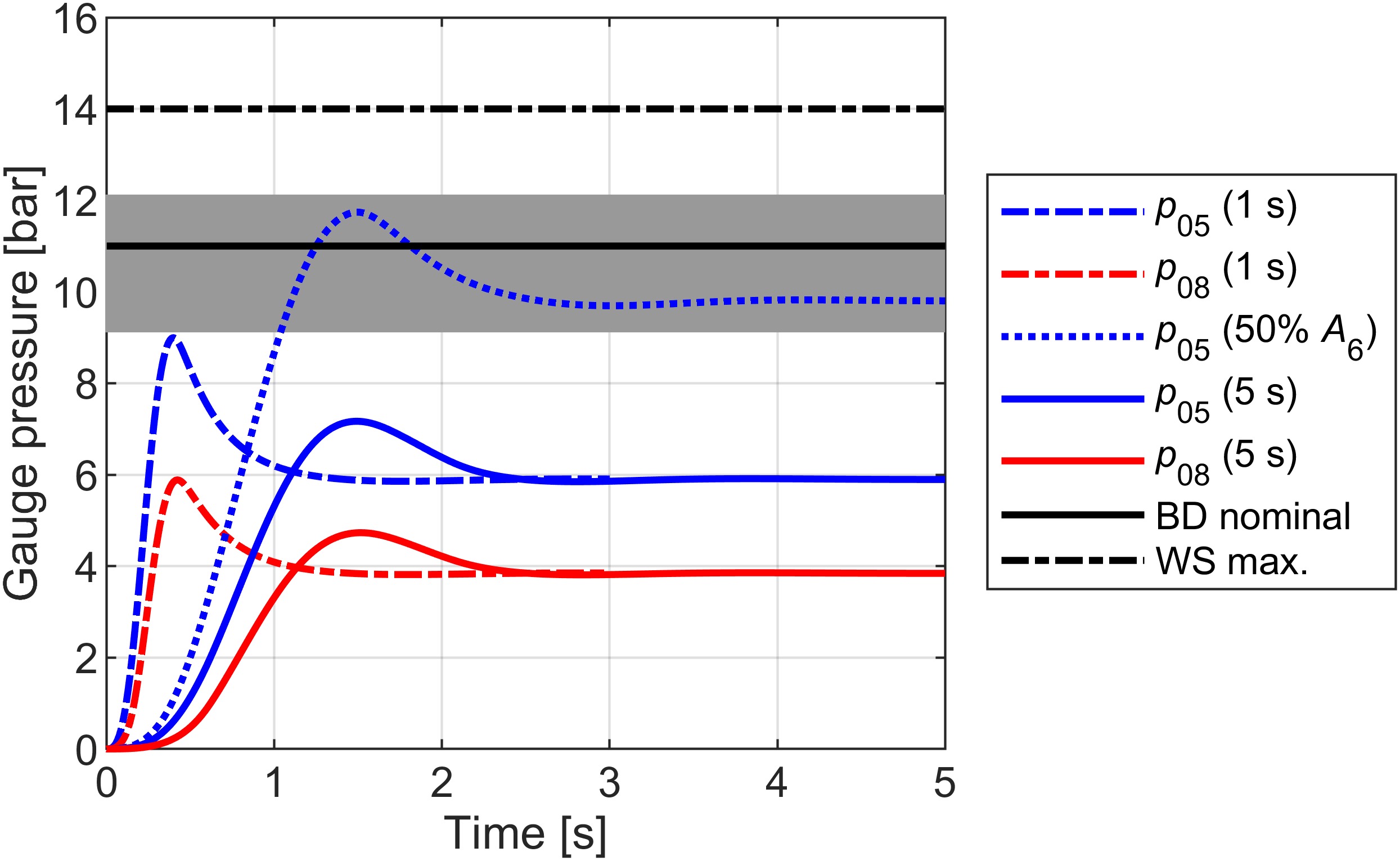
When the valve is modelled as opening in 1 s, the transient mass flow model predicts a peak pressure achieved upstream of the burst disk, p05, of approximately 10.0 bar, slightly greater than the 9.1 bar minimum burst disk rupture pressure. When the valve is modelled as opening in 5 s, the peak pressure is reduced to 7.2 bar, below the minimum predicted bust pressure by a margin of 1.9 bar (or approximately 25%). It is concluded that the minimum safe valve opening time is approximately 5 s for a burst disk with a nominal rated pressure of 11 bar.
An additional (dotted) line is plotted to show the effect of a 50% reduction in inlet feed nozzle area A6. Reducing the feed area significantly increases the pressure upstream of the feed nozzles (where the burst disk is located). For a valve opening time of 5 s the minimum burst pressure would be significantly exceeded. We see that the area of the inlet feed nozzles and distribution plate need to be carefully optimised to prevent unintended excursions in pressure during start-up. Whilst the trends of these results might be intuitive to someone skilled in the art of facility design, the sensitivities are perhaps unintuitive, justifying this modelling effort during the preliminary design phase.
Analysis of pipe heating requirement
Heat loss and heat pick-up in the pipework has a significant effect on the transient temperature characteristic of the facility. For metal effectiveness measurements of the NGVs, improving the inlet temperature stability of the facility (over time) is important. In this section we analyse the impact of using trace heating to pre-heat the air delivery pipework. In all cases, 1.5 m section of unheated pipe (station 5 to 6 in Figure 1) is intended to be installed between the working section and the upstream heated pipework, as a thermal break. This allows the working section to be accessed whilst the main pipework is brought up to temperature (the pre-heat time is several hours).
Figure 12a compares the mainstream feed temperature T0m for three configurations: unheated (initially 293 K) feed pipes; feed pipes pre-heated to 600 K; and significant sections of the working section (WS) internally insulated. The test period is shown by the dotted lines: between approximately 5 s and 70 s. The tank temperature (decaying due to isentropic expansion effect) is also shown.
Figure 12.
Feed temperature transients for: (blue) unheated pipework; (red) heated pipework; (green) heated pipework with substantial elements of the working section internally insulated. The black line indicates the tank temperature. (a) Temperature transient; (b) temperature ratio transient.
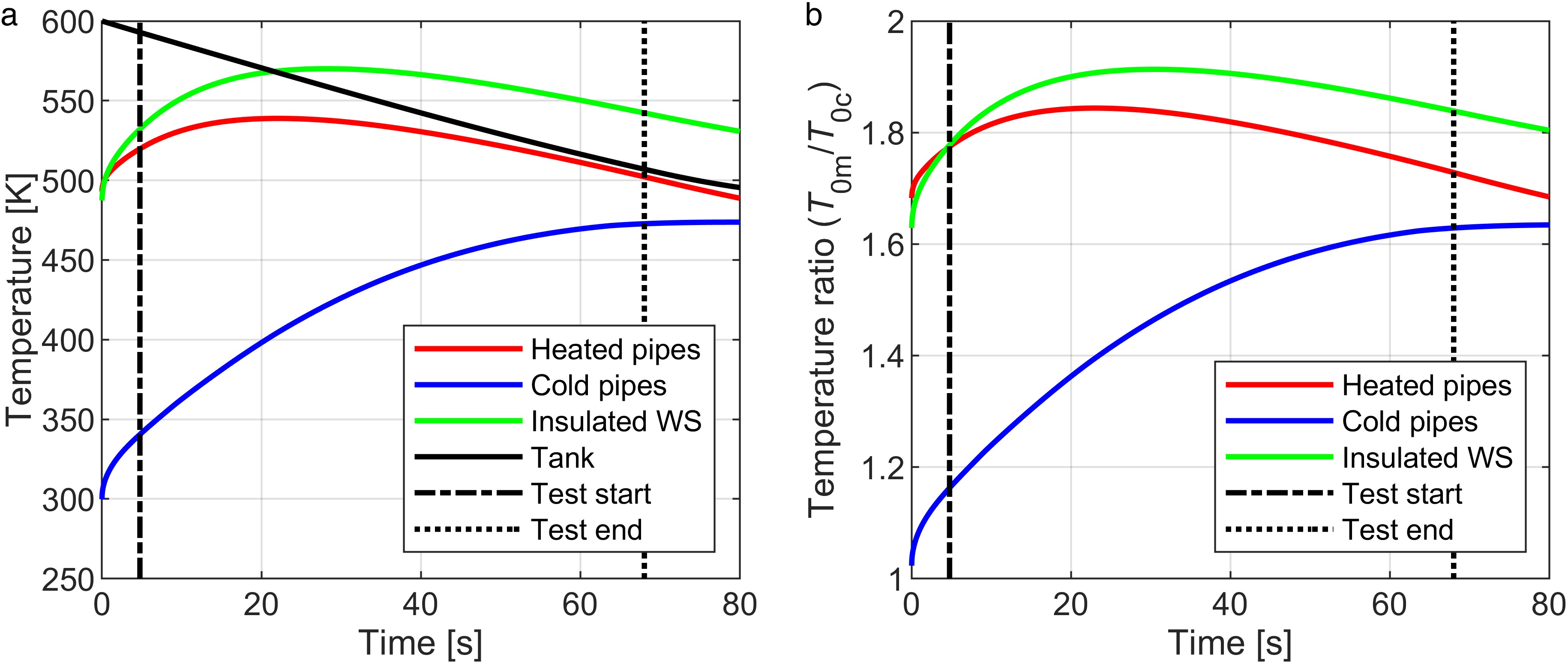
Figure 12b compares the mainstream to coolant temperature ratio for the three configurations. For unheated feed pipes (blue line) there is significant predicted variation in the mainstream feed temperature during the regulated period of the run, and the maximum temperature ratio is limited to T0m/T0c ∼ 1.6, well below the design target of T0m/T0c = 2.0. This is unsatisfactory in terms of the target operational capability of the facility. For heated feed pipes, the inlet temperature is stabilised during the regulated period of the run, and the maximum mainstream-to-coolant temperature ratio is substantially increased. During the run period the temperature ratio is in the range 1.7 < T0m/T0c < 1.8. When the pipework is pre-heated and substantial elements of the working section are internally insulated, the temperature variation is in the range 1.8 < T0m/T0c < 1.9, including a very substantial period of the run (between 20 and 40 s) in which the temperature ratio is close to the target and the variation is very small.
Transient response of test components
The transient response of a typical test component was also analysed. Here we consider a typical nozzle guide vane from a modern civil aero-engine. Temperature results are shown in Figure 13a and in a non-dimensional form in Figure 13b. The feed pipes have been pre-heated in the model and significant parts of the working section have been internally insulated to achieve the highest temperature ratio. Tw1 and Tw2 refer to the NGV external and internal wall temperature respectively and Trig the temperature of the working section internal walls upstream of the vanes. The vane Nusselt number (and associated heat transfer coefficient) has been scaled appropriately from engine to hot-core conditions (reduced fluid thermal conductivity with reduced temperature). Representative engine conditions have been taken from (Kirollos and Povey, 2016).
Figure 13.
NGV transient response (3.5″ venturi nozzle, 8″ regulator and insulated working section components): (a) transient temperature response; (b) non dimensional transient response.
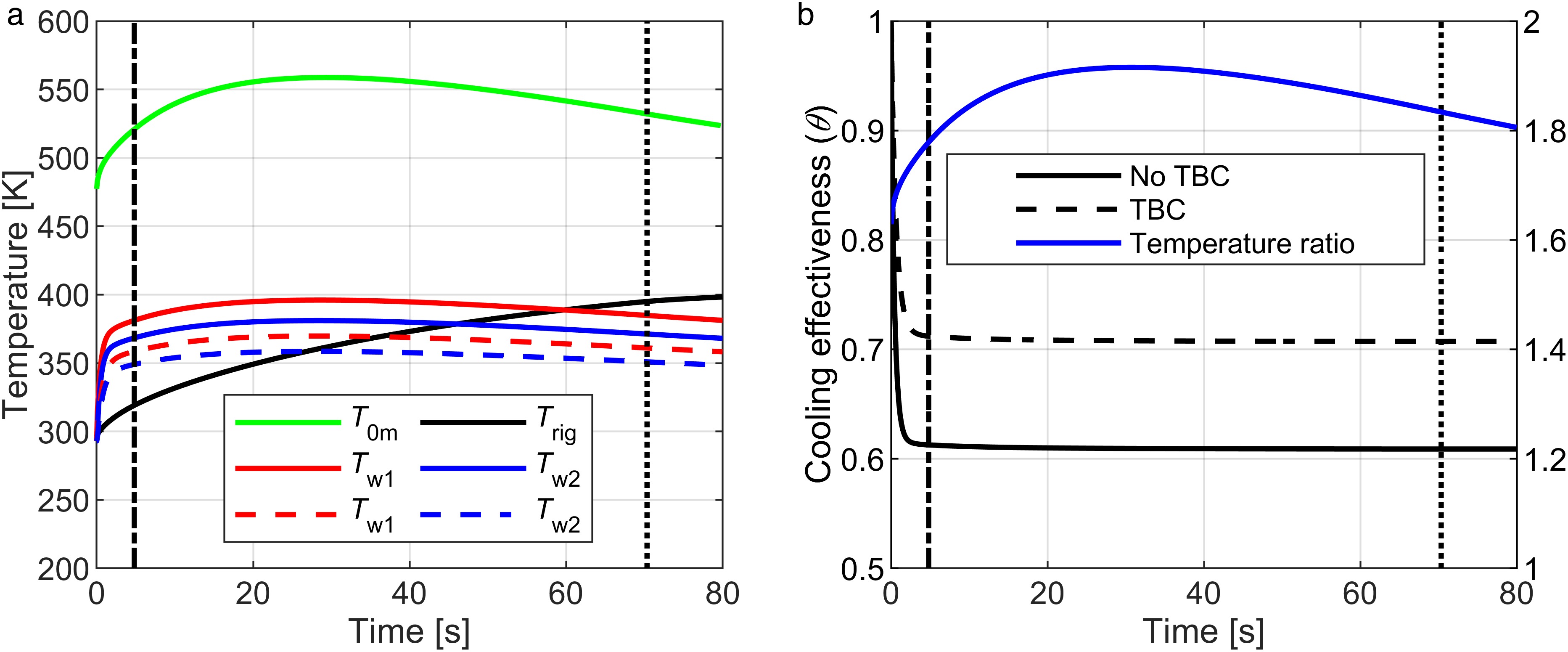
The vane temperature has been non-dimensionalised by Equation 8, and is shown in Figure 13b. As expected, the vane reaches its non-dimensional steady state (when normalised by the hot and cold gas temperatures) within the first few seconds of the test, and before the start of the nominal test window (5 s to 70 s). With pre-heated pipes and an internally insulated working section, even in absolute terms the predicted component external wall temperature is extremely stable, varying by less than 1 K in every 5 s period (typical averaging time for data) in the latter part (40 s to 60 s) of the run. Figure 13b also shows the effect of TBC (dashed lines) on the vane transient with the same coolant mass flow rate.
Effect on inlet conditions of a sequence of runs
A key operational consideration for the ECAT facility hot-core is the stability of the inlet temperature over a sequence of runs on a single day. The analysis code was run to simulate a typical sequence of runs on a single day, with a 1.5 h dwell-period between runs. This is typically longer than the tank recharge time (approximately 1 h) to allow for data-processing between runs.
Figure 14 shows the effect of multiple runs on the mainstream inlet total temperature with a partially insulated working section. The mainstream temperature increases only slightly with each subsequent run: the increase in maximum mainstream temperature between run 1 and run 6 is approximately 5 K, or approximately 1 K per run. We conclude that the temperature stability (repeatability) of the test conditions should be extremely good.

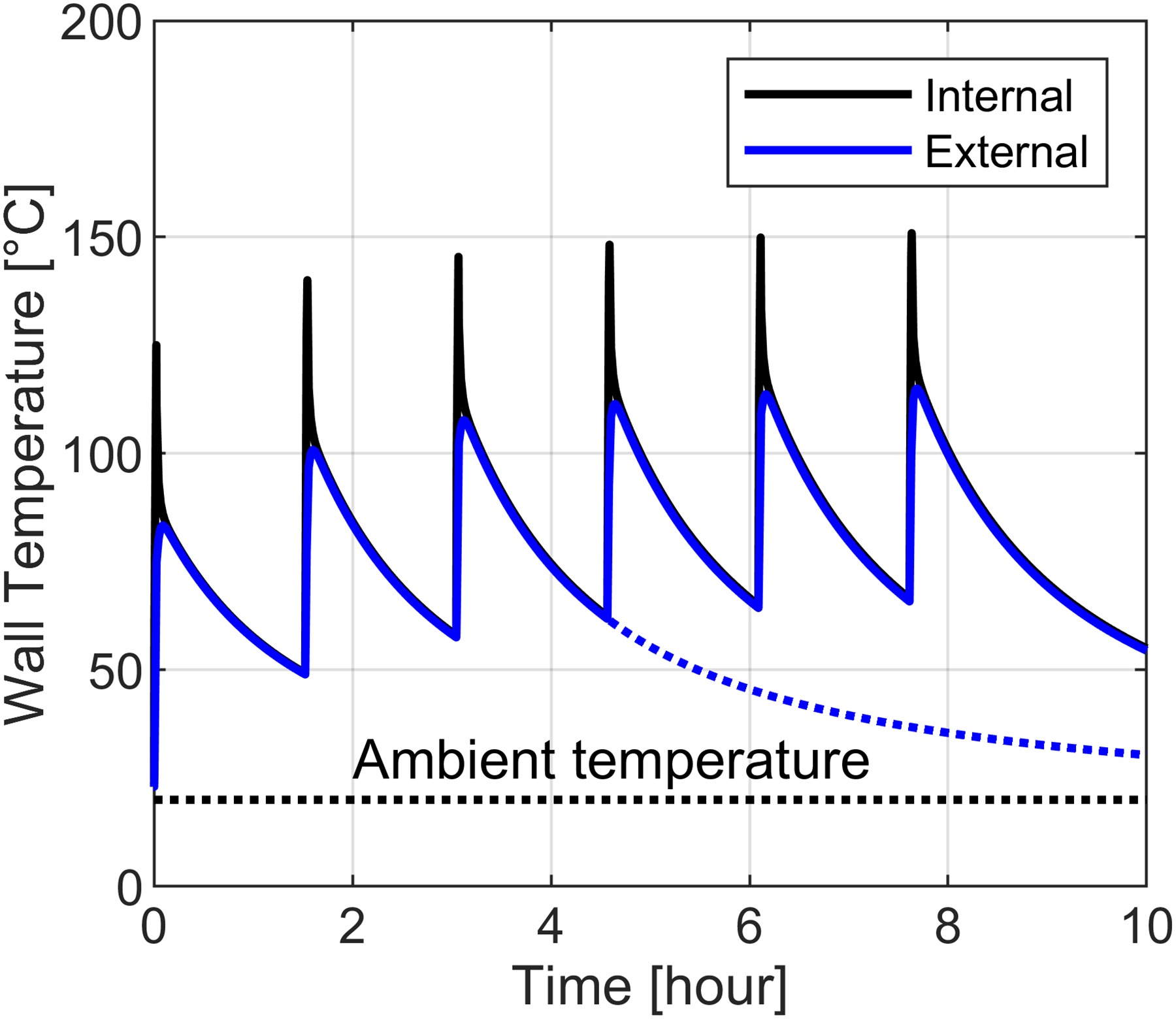
A practical consideration for facility management is peak temperature the main mass of the working section achieves during a test, as this dictates the time requirement for the working section to fall to an acceptable temperature to allow work on the facility (to allow operators to change the infrared camera position to view different vanes, for example).
The predicted working section internal and external wall temperatures are shown in Figure 15, for a working section with internal insulation on the most significant components. The internal wall temperature (black line) increases rapidly during a test, and then falls over several minutes to an intermediate temperature as the heat diffuses through the facility. In this period there is a rapid rise in the external temperature as the facility becomes approximately isothermal. The modelling assumes runs at an interval of 1.5 h. Cooling trends (by natural convection) are shown after run 3 and run 6 (a typical daily maximum).
Working section thermomechanical design
A principal design challenge associated with transient high temperature operation is the management of thermal stress induced the working section components. A typical working section pressure vessel has relatively thick walls (partly to meet safety factors at the design pressure, but also for mechanical stability related to component alignment issues). Thick walls exacerbate the temperature difference between inner and outer wall, however, and hence results in greater thermal stress. The working section design for the hot-core was based on the ECAT facility warm-core (Kirollos et al., 2017), and this was used as the basis for preliminary mechanical design.
Two different models have been used for thermal analysis. Preliminary design was undertaken by adapting the transient thermal model described previously to include thermal and pressure stress. We refer to this as the analytical thermomechanical model. More detailed finite element (FE) calculations were undertaken with a coupled transient thermal and linear stress analysis using Ansys Mechanical. Although all significant working section components have been analysed in this manner, in the following sections we confine our analysis to the axial stiffener which is an archetypal component so far as the thermo-mechanical issues are concerned.
Analytical thermomechanical model
In the preliminary design phase the transient working section model (including TBC coating or insulation and cladding on the inside) was extended to calculate the combined thermal and pressure stresses using the equations described by (Whalley, 1960) for a cylindrical vessel subject to an arbitrary radial temperature distribution. The equations are given in Appendix A for reference. To account for local stress concentrations around instrumentation ports etc., the component stress σc is taken as the von Mises stress multiplied by a stress concentration factor of 5.0, as recommended by (Price, 2007), and represents a realistic upper bound.
Material choice
The material considered for use in the axial stiffener component in this analysis was P460NH, a pressure vessel low alloy steel plate, see (British Standards Institution, 2017). Other more exotic materials could be considered with higher strength but will incur greater material and manufacturing cost. The yield stress of P460NH was taken as 375 MPa at 600 K, therefore to give a minimum factor of safety of 2, the maximum permitted component stress (σmax) was 187.5 MPa.
Thermal boundary conditions
To determine the thermal boundary conditions for the thermomechanical model, the warm-core ECAT working section was instrumented with surface thermocouples. Thermocouple beads were attached to the surface with silver conductive paint. Local heat transfer coefficients at the thermocouple locations were calculated using the method described in (Michaud and Povey, 2018). The heat transfer coefficients derived from warm-core ECAT measurements were then scaled to hot-core conditions using conventional scaling rules (Nu–Re correlations, for example).
The bulk heat transfer coefficients were calculated by considering the mainstream temperature drop through the working section, in the same manner as for the evaluation of the tuned parameters in the transient thermal model. To decouple the mechanical analysis of the working section from the facility temperature transient predictions (to avoid cascading errors), the flow temperature was assumed to be at 600 K for 80 s. This is a worst-case scenario in terms of the thermal load on the components.
Results
The radial variation of von Mises stress (due to pressure and thermal loading) for the outer wall of the axial stiffener component is shown in Figure 16, for both uninsulated and insulated (inner wall) components. The insulation considered was 2 mm thick calcium-magnesium silicate sheet (k = 0.24 W/mK), mechanically protected with 1 mm thick stainless steel cladding. The axial stiffener is a 30 mm thick rolled steel ring in the warm-core ECAT working section (on which the initial analysis was based). The radial stress distribution is taken at the time step which gives the maximum stress in the distribution. We see that in the uninsulated case the von Mises stress on the inner and outer radial limits of the wall significantly exceeds the allowable design stress (187.5 MPa). The effect of a 2 mm thick insulating layer is sufficient to reduce peak stress to approximately 93 MPa, giving a safety factor of 4.
Figure 16.
Maximum von Mises stress distribution for insulated and uninsulated working section components. Pressure and thermal loads.
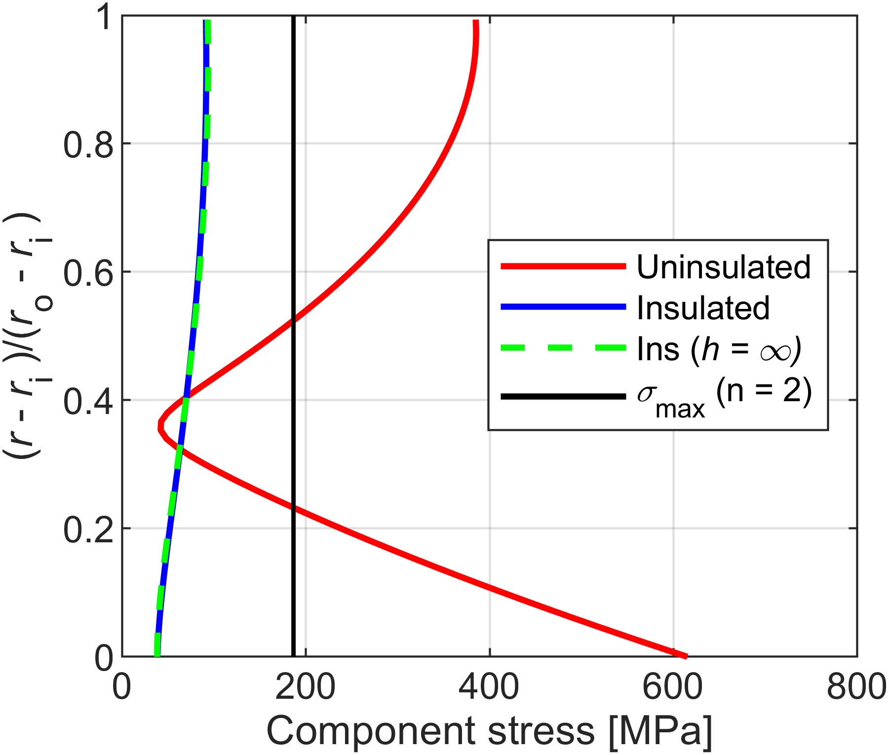
As a check on sensitivity to the heat transfer coefficient, a fixed wall temperature of 600 K was applied at the external surface of the cladding. This is equivalent to an infinite heat transfer coefficient (h = ∞) on the inner wall of the vessel. As shown in Figure 16, the predicted stress levels in the metal are essentially unaffected. This is explained by the relatively low thermal mass of the (1 mm thick) steel liner and the relatively high thermal resistance of the insulation. The conclusion is that solutions for insulated components are insensitive to the particular heat transfer coefficient.
Comparison of peak stress for different wall thicknesses
Reducing the thickness of components can reduce thermal stress on components due to rapid transient heating, and this was investigated using the analytical transient thermomechanical model. Three thicknesses were considered; 30 mm (as per warm-core ECAT), 10 mm and 5 mm, and the von Mises stress radial stress distribution is shown in Figure 17 for combined (pressure and thermal) loads and pressure only load. Reducing wall thickness reduces the thermal stress on the component but increases the stress due to internal pressure. In this case all considered thicknesses fail, and therefore the optimum solution to handle the thermomechanical loading is by insulating the component internals.

Detailed FE stress analysis
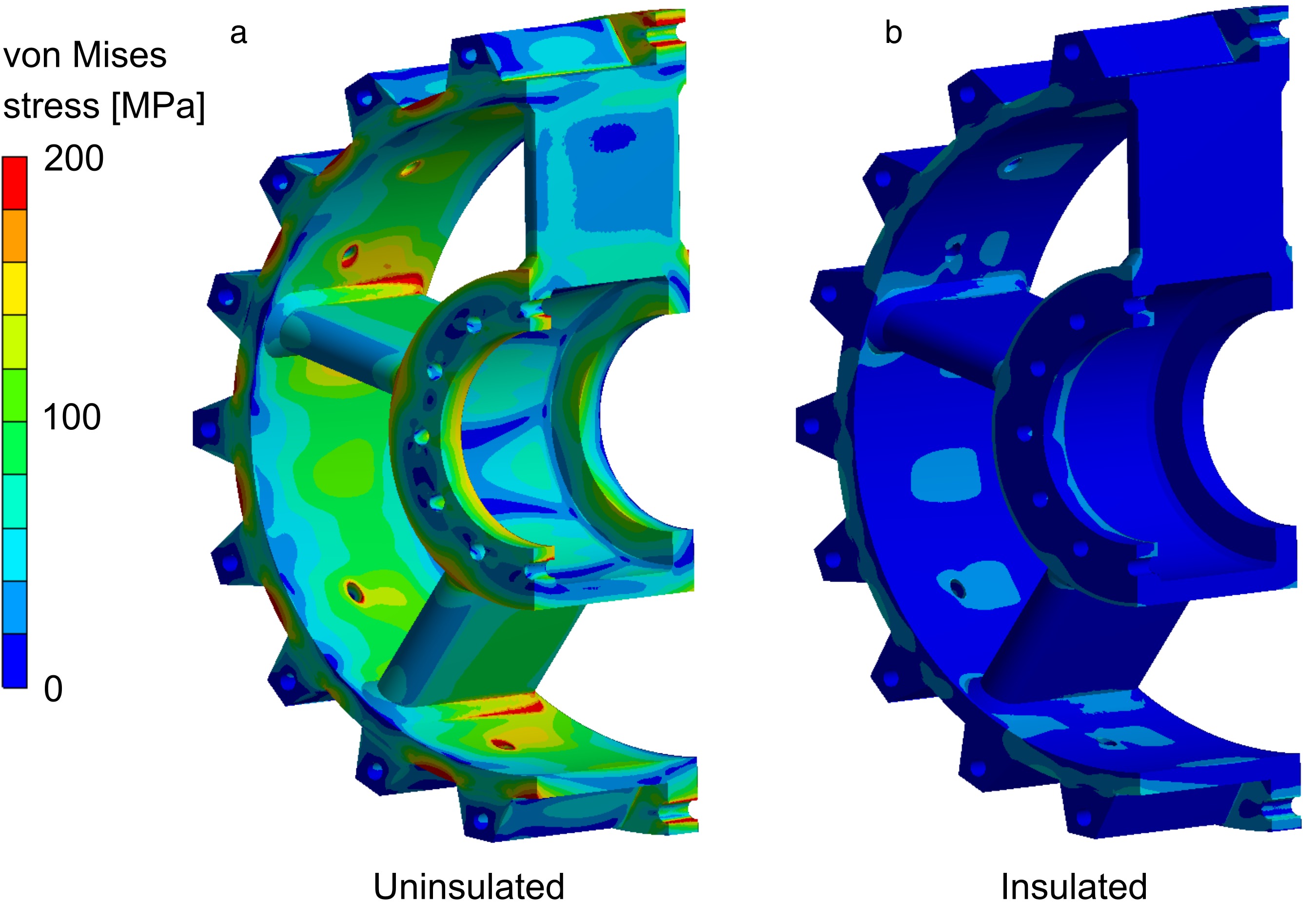
Further analysis was undertaken using a coupled transient thermal and linear elastic stress analysis using Ansys Mechanical. The axial stiffener component is presented as an example in Figure 18 and compares the uninsulated (a) and insulated (b) von Mises stress distribution after 80 s. Significant portions of the model go beyond the yield stress of the material when uninsulated. The peak stress, approximately 450 MPa, is within the upper bound calculated by the analytical thermomechanical model (600 MPa). The insulated component (b) shows significantly reduced stress. Rather than model the insulation and cladding layer directly in FEA, which would need a very high number of cells, the Matlab transient thermal model was used to calculate temperature at the boundary between the insulation and the component metal, and this was used as the FEA thermal boundary condition. As in the previous analysis, a constant internal wall temperature of 600 K was used as the thermal boundary condition at cladding surface.
Conclusion
Design calculations for a substantial upgrade to the existing warm-core ECAT (Engine Component AeroThermal) facility at the University of Oxford have been described. The purpose of the upgrade is to extend the functionality of the facility from warm-core operation to hot-core operation. The new development will allow very-high-TRL analysis of the aerothermal performance of hot-section components (most commonly—but not exclusively—the HP NGV) to be conducted in a university environment. The increased mainstream inlet temperature of the facility will enable full matching of non-dimensional parameters to the values at engine conditions.
A low-order transient heat transfer model was developed, and used to inform key facility design decisions, including: the necessity of external lagging of the feed pipe system to stabilise the inlet temperature transient to the facility; the necessity of pre-heating on the air supply system to stabilise the inlet temperature transient; the sizing of the limiter and regulator system to maximise run time whilst giving manageable safety-case scenarios; the necessity of internal insulation in the working section to manage transient thermal stress. Other operational metrics were assessed, for example the predicted metal effectiveness transient of typical engine parts, and the cooling characteristic of the facility for typical test sequences.
Two low-order flow models of the feed system were developed: a steady state solver to optimise the run time and feed system areas (pressure regulator size and choked venturi throat diameter); and a transient solver to understand the behaviour of the facility during start up. Results from the transient solver informed requirements for minimum opening time for controlling valves and allowed more sophisticated analysis of the pressure safety system (which must be designed with a margin with respect to transient pressure excursions).
These low-order models have been extensively validated using experimental data from the existing ECAT facility warm-core and provide interesting insights not normally available at this point in a facility design exercise. Whilst some of the trends may be intuitive to someone skilled in the art of facility design, the sensitivities are perhaps unintuitive, justifying this modelling effort during the preliminary design phase.
The mechanical design of the working section is also discussed, the principal design challenge being the high transient thermal stress due to rapid heating of the working section components. The design was optimised by extending the transient heat transfer model to analyse stress due to pressure and thermal gradients, before detailed design calculations were carried out using a transient finite element code. Boundary conditions for both models were obtained from measurements in the ECAT facility warm-core. Thermal stress was found to be significantly greater than pressure-induced stress. The modelling results showed that an effective way of mitigating high thermal stress regions was to internally insulate certain working section components. This has the additional benefit of both increasing and stabilizing the mainstream temperature characteristic, thus extending the operating envelope of the test facility.
It is hoped that the detailed, validated, low-order design approach described in this paper, developed during the design and development of numerous successful complex facility developments, can form an example of good practice for others in the community developing test facilities of similar scope. The development of the upgraded facility will also be of interest to those following the trend of very-high-TRL research in university environments, developed for accurate aerothermal assessment of new concepts at highly engine-realistic conditions.
Nomenclature
Romans and greeks
A
Area, m2
Bi
Biot number
cp
Isobaric specific heat capacity, J/kgK
cv
Isochoric specific heat capacity, J/kgK
D
Diameter, m
E
Elastic modulus, Pa
g
Acceleration due to gravity, m/s2
h
Heat transfer coefficient, W/m2K
K
Ratio of outer to inner radii (ro/ri)
k
Thermal conductivity, W/mK
L
Arbitrary length scale (0.1 m), m
M
Mach number
m
Mass, kg
Mass flow rate, kg/s
Nex
Tuned parameter (external convection)
NP
Tuned parameter (pipe model)
NT
Tuned parameter (tank model)
NWS
Tuned parameter (working section model)
Nu
Nusselt number
n
Number of radial nodes
Pr
Prandtl number
p
Pressure, Pa
Q
Heat energy, J
Ra
Rayleigh number
Re
Reynolds number
r
Radius, m
ri
Inner radius, m
ro
Outer radius, m
T
Temperature, K
V
Volume, m3
α
Coefficient of thermal expansion, 1/K
η
Adiabatic film cooling effectiveness
ϴ
Cooling effectiveness
μ
Dynamic viscosity, Pa s
ν
Kinematic viscosity, m2/s
ν
Poissons ratio
ρ
Density, kg/m3
σ
Stress, Pa