Introduction

Linear cascades are routinely used to analyse aerodynamic performance of turbine components. Heated compressed air is passed through the test cascade, optionally with cooling flow, to conduct heat transfer measurements. Thin film gauges or infra-red thermography are used to record high frequency surface temperature measurements, without impeding design form or profile. The data is commonly post-processed using the impulse response method (Oldfield, 2008). In most practical heat transfer applications, the evaluated geometry is not simply a planar surface. In such cases, the 1D Cartesian assumptions used to define the impulse response rarely hold. As a result, direct application of the traditional impulse response method leads to errors in the analysis. Particular importance is given to the handling of freeform surfaces, which are especially prevalent in turbine components and casings. The impact of geometric curvature is quantified in this paper and a new radial 1D method is presented to enable accurate heat transfer analysis of non-planar systems.

Buttsworth and Jones (1997) examined the effect of radial convection on both convex and concave geometries. They demonstrated an approximate Heat Transfer Coefficient (HTC) correction which altered a flat plate equivalent HTC by a simplified material dependent curvature term. The method was tested against the analytic solutions defined by Carslaw and Jaeger (1947) which are discussed in the following section, Equations 9 and 10. Buttsworth and Jones’s truncated series assumed negligible heat penetration depth and the error was shown to vary significantly depending on the Biot and Fourier number. The method was most reliable on concave geometry but is only valid for very short duration tests.

In 2008 Martin Oldfield evaluated the cylindrical surface temperature, for unit step heat flux, on the convex case only. This paper now fully defines the cylindrical impulse response functions, using the Carslaw and Jaeger analytic results, to allow direct implementation for both the convex and concave cases. The modified filter functions enable the error in the planar assumption to be quantified and avoid the need for flat plate approximations when analysing heat transfer in curved and freeform geometry.

Cylindrical 1D heat equation

When analysing the effects of curvature, the radial heat flow in a cylindrical system can be used. Freeform surfaces can be accurately approximated by a single curvature, simply taking the mean principal radius. The 1D assumptions are then valid but are subject to additional criteria. Firstly, the radial heat flow must be significantly greater than the axial and circumferential heat flow.

Secondly, when evaluating heat flux into the cylinder, the normal semi-infinite behaviour defined by Schultz and Jones (1973) cannot be assumed as r→0. Similar to heating a flat plate from multiple sides, which forces the 1D semi-infinite depth to be half the plate thickness; the semi-infinite duration in a cylinder is limited by the penetration depth to its centre and thus limited by the minimum radius of curvature. If these two assumptions are valid, along with the standard assumptions required by impulse response analysis (isotropic, constant uniform material properties, linear time invariant, zero initial state), the heat equation in a cylindrical coordinate system can be used to define the curvature basis function.

Taking the Laplace transform with zero initial conditions, Abramowitz and Stegun (1972), Equation 2 can be rearranged to give a second order modified Bessel differential equation Carslaw and Jaeger (1947).

Equation 3 has the well-known general solution given by the modified Bessel functions.

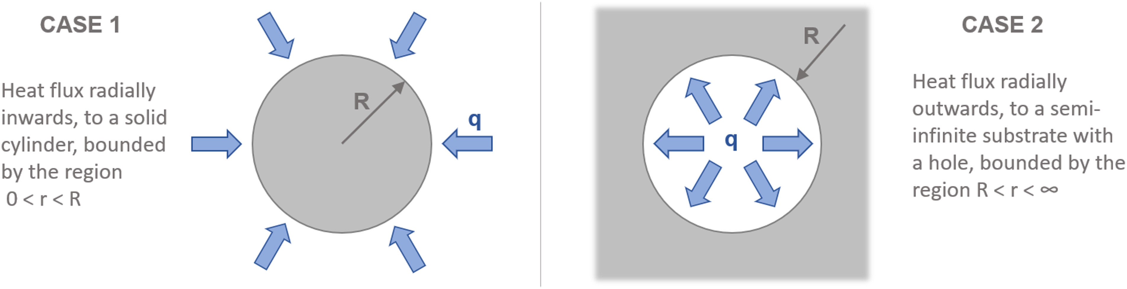
Two separate conditions, shown in Figure 1, must be considered when solving Equation 4.

Figure 1.

Definition of the two radial heat flux cases that must be considered, showing the bounded region in grey and associated boundary heat flux condition in blue.

Cylindrical unit step heat flux

Following the same methodology as the 1D planar case, the time domain form can be found by inverting the Laplace solutions from Equation 5. Carslaw and Jaeger (1947) presented the cylindrical solutions for unit step surface heat flux. Applying the boundary condition q(R,s)=1/s=−kdϕ/dr and using the following properties of the modified Bessel functions.

The Laplace domain solutions for unit step heat flux, applied to a region bounded by a cylinder of radius R, are given by

Inverting these solutions, the time domain form can be found. Case 1, radially inward heat flux to a solid cylinder, bounded by the region of radius 0<r<R.

Case 2, radially outward heat flux, to a semi-infinite substrate with a hole, bounded by the region of radius R<r<∞.

The solution of the second case uses the asymptotic expansion of the modified Bessel function of the second kind Kn(r,s). This expansion is most accurate for small values of αt/R2. Carslaw and Jaeger (1947) recommend a typical limit of αt/R2<0.02. In cases where this limit is exceeded, a large time approximation is available via Equation 11 and has an error term O(R2/αt). In the application of 3D printed SLA, for long test durations to approximately 20 s, the small value limit is not exceeded and the above expanded form in Equation 10 should be used.

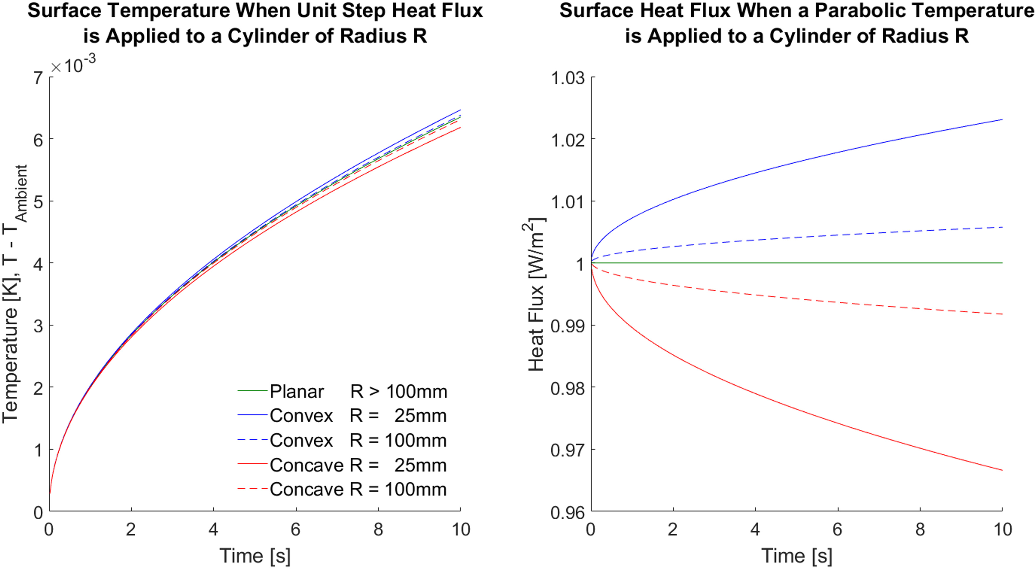
Figure 2 shows the impact of the radius of curvature on the surface temperature necessary to achieve unit step heat flux. Two analyses were performed, the first applied unit step flux then observed the change in surface temperature at different curvature radii. The second applied the planar analytic, constant flux, surface temperature solution defined by a parabolic surface temperature T(t)=4αt/πk2, then observed the change in heat flux in the material. In SLA, surfaces with radii greater than 100 mm show only 0.5% difference in surface heat flux. Above this threshold, surfaces could reasonably be considered planar because there is negligible modification to the surface temperature and flux distribution. However below this threshold, particularly in high curvature cases, a notable heat flux error is seen. The planar threshold is material and test duration dependent and should be evaluated on a case by case basis. For radii below the threshold value, the curvature effects should not be ignored and the system behaves notably different to a planar 1D case.

Figure 2.

Effect of curvature on the surface temperature and heat flux for 1D unit step solutions, q(t)=U(t), T(t)=4αt/πk2, in a SLA substrate.

The Carslaw and Jaeger (1947) solutions in Equations 9 and 10 are quite involved and implementation of these formula is non-trivial. The infinite series expansion terms should be added iteratively, truncating the series only once the magnitude of the terms fall below a negligible value. The number of terms required is material and geometry dependent so must be evaluated on a case-by-case basis. Once the surface temperature solution is known, the curvature corrected impulse response can be defined using the methods in the following section.

Radial 1D impulse response method

Assuming that the test behaves as a 1D linear-time-invariant, isotropic, semi-infinite system; the thermal impulse response method can be used. The response function FTq is defined by a known analytic solution pair Ta and qa, then later used to calculate the measured heat flux qm from the measured surface temperature Tm (Oldfield, 2008). Historically all thin-film gauges, or thermal camera pixels, are assumed to behave identically and the same planar response filter is applied uniformly to all data in parallel. Curvature compensation requires that each thin-film or pixel be considered unique, having its own specific curvature dependent filter. Thus curvature correction prevents parallel processing of multiple thin-films or thermography data. This computational cost affects every test run and may not be viable in high density thin-film applications. In such cases, a fixed range of filters for differing radii can be defined, then an interpolation function used to correct the response output for a particular curvature. In this way the computational cost is only increased by the number of interpolation references, rather than the number of gauges or pixels to be post-processed. The input analytic solution Ta(r,t) is simply taken from Equation 9 or Equation 10, depending on whether the case is concave or convex, then r selected for the desired curvature radius and qa(r,t) set as the unit step U(t).

In the preceding publication (Baker and Rosic, 2022), the authors showed that multilayer effects have notable impact on the accuracy of thin-film data analysis. Full implementation of curvature correction necessitates that each of the reflected terms be corrected for their particular interface radius. In the case of many layers, this calculation is computationally very expensive. However, if the thin-film thickness Δx (typically <100μm) is significantly less than R, curvature correction can be uniformly applied. This is achieved via a compound response function, stacking the multilayer and curvature effects. A temperature only response is generated that maps the planar case to the radial case, Equation 14, then applied to the unit step multilayer temperature solution. The final heat flux impulse response, Equation 15, is calculated using the modified analytical input and allows direct post-processing of the measured surface temperature via Equation 13.

Although the effects of curvature and multiple layers can be compensated, two significant limitations of the impulse response remain: the inability to handle back surface boundary conditions and the failure to model temperature dependent material effects. In such cases a 1D numerical scheme must instead be used. An adapted scheme is defined below, extending the numerical capabilities to handle temperature-varying multilayer curvature effects in non-planar geometry.

Radial 1D Crank-Nicolson method

The 1D Crank-Nicolson method was previously presented as an alternative post-processing solution to avoid the time-invariant limitations of the impulse response (Baker and Rosic, 2022). This method can also be modified for use in a cylindrical system for curvature correction. Mori and Romão (2016), and Duda (2016), presented a polar implementation of the scheme for a single material. The bulk of the multilayer solver can be updated to follow this solution which requires a modification to the b and c vectors only. The interfaces for heat flux continuity can be approximated by using the existing relation from the planar 1D case. This simplification has little impact on the result, particularly if the nodal count in the simulation is high. The following modifications are required to the Crank-Nicolson method to allow use in a cylindrical system. The resulting penta-diagonal matrix can be solved using the algorithm described by Askar and Karawia (2015) without modification.

The single material cylindrical Crank-Nicolson solution is defined by Equation 16.

This can be rearranged to separate the two temporal steps: tm and tm−1. These solutions are very similar to the 1D planar case, with only one additional ±α/4rΔr term in the spatial i+1 and i−1 positions.

Which can be combined with the material interface factors and expressed more concisely in matrix form.

where: ∗ indicates a boundary interface and,

The modified curvature matrix now includes the location specific value r. Similar to the modified impulse response, a multiple solution interpolation can be used, allowing parallel analysis of many differing locations on the test article. The numerical solution can be applied to both convex and concave cases by simply setting the respective values of r in the domain. Similar to the 1D planar case, the numerical Crank-Nicolson method offers a solution beyond the semi-infinite duration if a back boundary condition is known. It additionally allows time or temperature dependent material properties to be handled, offering an alternative to the limitations in the impulse response. Preference should be given to the impulse method for post-processing if the required assumptions hold, due to the computational speed compared to a numerical approach.

The cylindrical solution provides a significant improvement to traditional 1D planar analysis, but still assumes heat flux in the surface normal direction. Applications that produce high axial or circumferential temperature distributions are not well suited to this methodology. Similarly, geometries with regions of very small radii, such as the trailing edge of turbine blades, do not satisfy the curvature semi-infinite criteria and cannot use this method. These cases are not considered radial-1D and should be modelled using 3D numerical techniques. When handling sharp geometric features such as edges or corners, Jiang et al. (2015) presented an efficient superposition method to process the differing heat penetration directions. This method is effective at handling corner geometry and is recommended where these features exist in the geometry. The discussed curvature corrected methods, the impulse response and numerical Crank-Nicolson scheme, both require that the radius of curvature at each measurement point is known. This curvature value must be extracted from the test geometry in order to use these models, a robust method to calculate the point-wise surface curvature on complex freeform geometry is therefore defined below.

Surface curvature calculation

3D CAD geometry is increasingly common in engineering practice. These design software allow complex freeform surfaces to be constructed, often via spline or mesh specification. Surface or volume mesh definitions of CAD models are widely used for numerical simulation or for direct manufacture via 3D printing. The rise of additive manufacture has led to increasingly complex designs and neutral format surface topology files are routinely used to specify the surface data. The files segment the surface into the many faceted 2D shapes, defining elements by vertex and facet connectivity. Stereolithography files (.STL) are among the most common and use triangulation to capture surface curvature and can be exported from most CAD or meshing software.

Rusinkiewicz (2004) presented an algorithm to calculate the curvature at each vertex of an STL file. The algorithm takes a vector of face and vertex data defined in the STL, parses the surface normals, then returns the principal radii of curvature at each vertex. Using default settings, some CAD packages do not automatically output unified normal files. The surface are often defined by how the user first constructed them, meaning that adjacent surfaces may have normals that point in opposing directions. In such cases, the normals must first be unified so that they are all aligned outwards from the geometry. Without this step, significant error is introduced to the area weighted vertex normal calculation due to the opposing adjacent facet normals. Exporting an STL from a meshing package e.g. ICEM, this unification step is usually applied by default. It is therefore recommended that mesh exported STL files be used rather than those from native CAD.

Johnson (2011) provided MATLAB code, available from the Mathworks Exchange, to read standard ASCII or binary STL files. Combining the read codes with the MATLAB implementation of Rusinkiewicz’s curvature algorithm (Shabat and Fischer, 2015), the surfaces of any freeform CAD model can be evaluated easily. The proposed methodology uses an equivalent cylindrical system, converting the freeform surface to a single curvature value found by taking the mean of the vertex principal values. Figure 3 outlines the calculation process and Figure 4 shows the resulting curvature map on an example linearised turbine Nozzle Guide Vane (NGV).

Figure 3.

Overview of the surface curvature calculation method from the initial CAD geometry through mesh face and vertex normals to final mean principal radius of curvature, κm=1/2(κ1+κ2) Crane (2021).

Figure 4.

Left: ICEM mesh of a 3D linearised turbine nozzle guide vane geometry used for STL definition of the geometry. Right: the curvature map of the main blade surfaces after processing with Rusinkiewicz’s algorithm.

Radial 1D validation

The test article chosen uses a linearised turbine NGV. This geometry contains all features of interest: planar faces, variable curvature, convex and concave surfaces, small radii and regions that violate the semi-infinite criteria. The new radial procedure was validated by comparison to a 3D transient thermal analysis completed in ANSYS. A constant flux boundary condition was applied to the solid domain only, which replicates the unit step flux solutions discussed in Equations 9 and 10. The unstructured tetrahedral mesh, shown in Figure 5, used 21 inflation layers on all heated boundaries to accurately capture the thermal gradient and heat penetration normal to the surface.

Figure 5.

Monitor point locations used in the ANSYS simulation and a section through the NGV ICEM mesh, showing the inflation layers and tetrahedral core.

A uniform step in surface heat flux (104W/m2) was applied to all main passage faces and the time-varying temperature profile recorded for the Figure 5 monitor locations with differing curvature. These monitor points offer a controlled replica of the surface temperatures that could be measured by a thin-film gauge during an aerothermal test. The simulation was run for 10 s, corresponding to the semi-infinite duration of the geometry endwall, this final surface temperature profile is shown in Figure 6. A surface STL file was extracted and used to calculate the effective curvature at each vertex, using the process defined in Figure 3. The radial 1D analytic temperatures, Equations 9 and 10, were compared point-wise to the monitor results. The trailing edge region of the geometry was removed from the analysis because it has a radius of curvature too low to be considered semi-infinite. The simulation results confirm that the convex regions: the blade leading edge and suction surface, heat up faster than a planar case and the concave regions: the pressure surface and blade root radii, heat up notably slower. This is due to the convergent or divergent radial heat penetration, either concentrating or diffusing the heating effect.

Figure 6.

ANSYS solution of the main blade passage surface temperatures at the end of the 10 s simulation with applied 10⁴ W/m² surface heat flux and initial temperature 20 °C.

Figures 7 and 8 compare the temperatures in the ANSYS simulation and the analytic solutions. The error between the ANSYS surface monitor points and the analytic temperature is less than 1 K for the curvature corrected solutions. Significantly higher errors are seen when using the planar 1D approximation. Only the blade root radii, where the curvature is most extreme, is any significant error seen in the curvature solution. This is caused by subsurface diffusion of heat from the adjacent regions, thereby reducing the accuracy of the 1D radial assumption. Diffusion from the endwall and the blade reduces the effective volume into which the heat is dispersed. The surface thus heats up faster than the 1D cylindrical prediction. In these cases of extreme curvature, it is required to modify the 1D cylindrical calculation. This should be done by applying an equivalent radius of curvature in the formula rather than the true value. Several different equivalent radii were tested, in this application, selecting 8.0 mm demonstrated the best surface temperature agreement with the numerical simulation.

Figure 7.

Transient surface temperatures for the 1D analytic curvature solutions and monitor points in the 3D NGV ANSYS simulation for unit step surface heat flux 10⁴ W/m². The analytic endwall case is equivalent to the 1D planar assumption.

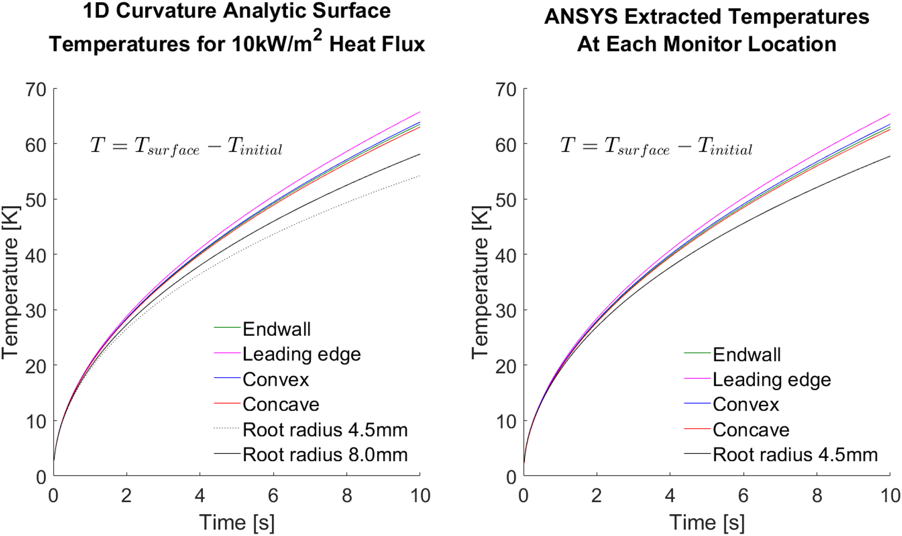
Figure 8.

Comparison between the extracted ANSYS monitor point temperatures and the analytic solutions for both the 1D planar and 1D curvature corrected cases.

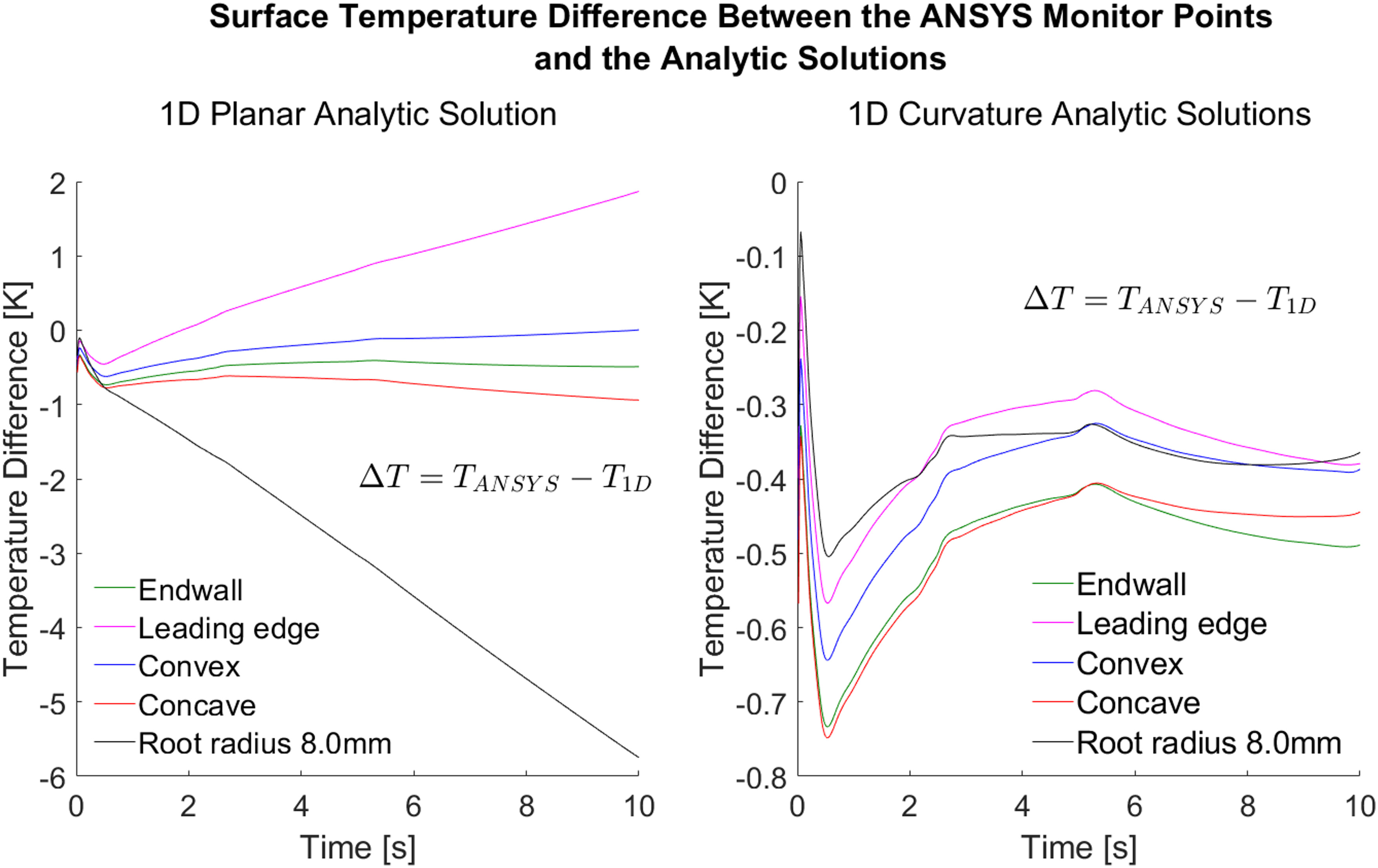
The largest temperature difference in Figure 8 is seen immediately, at the start of the simulation, this behaviour was also seen in the previous multilayer 1D numerical analysis (Baker and Rosic, 2022). The numerical error is largest when thermal gradients are first being established in the spatial simulation. The difference between the ANSYS and analytic solutions then stabilises, showing a near constant offset in the latter part of the simulation. This offset is most likely caused by the discrete domain in the ANSYS simulation, and the use of a subsurface inflation layer temperatures to set the constant −kdT/dr heat flux boundary condition.

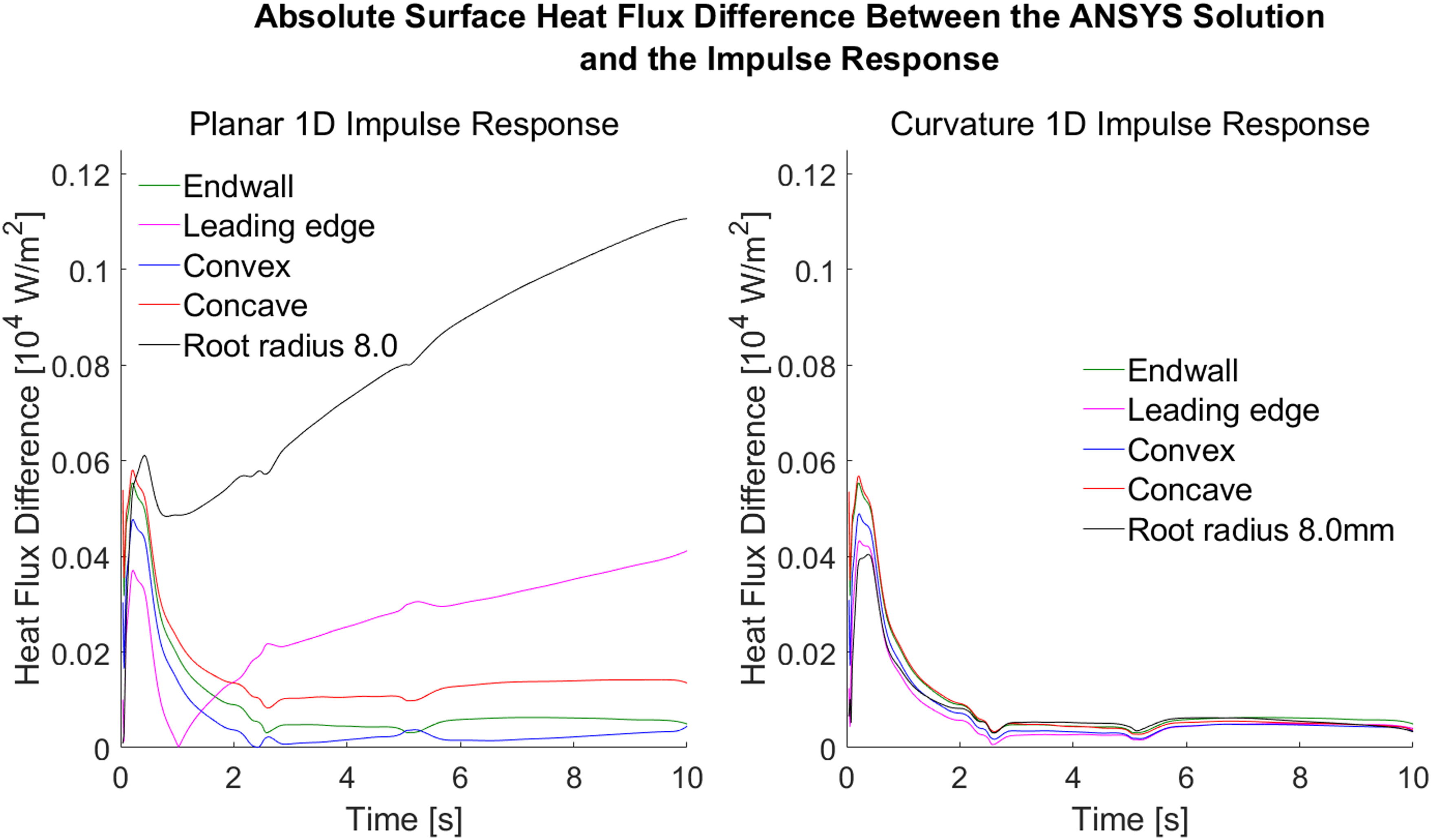
Figures 9 and 10 compare the heat flux in the ANSYS and analytic cases. The impulse response function has been calculated for the 1D planar and 1D curvature solutions, using the mean principal radius of curvature as the single curvature value in each location. The separate filters where then applied to the extracted ANSYS temperatures in turn to evaluate the error in traditional planar impulse response assumptions. The high curvature regions are the most effected, with large discrepancies for the root radius (11%) and leading edge (4%). The analysis also shows notable error (1.5%) across large parts of the concave blade surface. The error caused by the planar assumption increases with time and curvature effects must be considered when operating long duration tests. The curvature corrected solutions are notably more accurate, being uniformly within 1% once the initial transients subside. The peak error is likely caused by initial numerical inaccuracies in the ANSYS simulation temperature as the thermal gradient is first established. The impulse response convolution is affected by the full time history, so these initial transients also affect the latter part of the analysis.

Figure 9.

Calculated surface heat flux when applying the impulse response to the extracted ANSYS monitor point surface temperatures.

Figure 10.

Comparison between the impulse response calculated surface heat flux and the 10⁴ W/m² ANSYS boundary condition, showing the improved accuracy of the curvature corrected solutions.

The point-wise validation simulates an aerothermal test with thin-film gauges, returning a low number of discrete time-series surface temperature measurements in order to find the associated heat flux. For improved resolution, many experimentalists now turn to infra-red thermography, allowing them to better define the spatial variation in surface heat transfer. In thin-film applications, the location of the measurement is known because the gauge position was designed in the film manufacture. In thermal camera applications, the pixel location is not known because the camera alignment is arbitrarily defined, or even moved on each test. To apply the curvature correction methods of this paper to thermography, the camera and geometry must first be registered to allow the correct curvature to be defined at each pixel. The following section introduces a thermal camera registration technique, enabling curvature correction of infra-red data.

Thermal camera registration

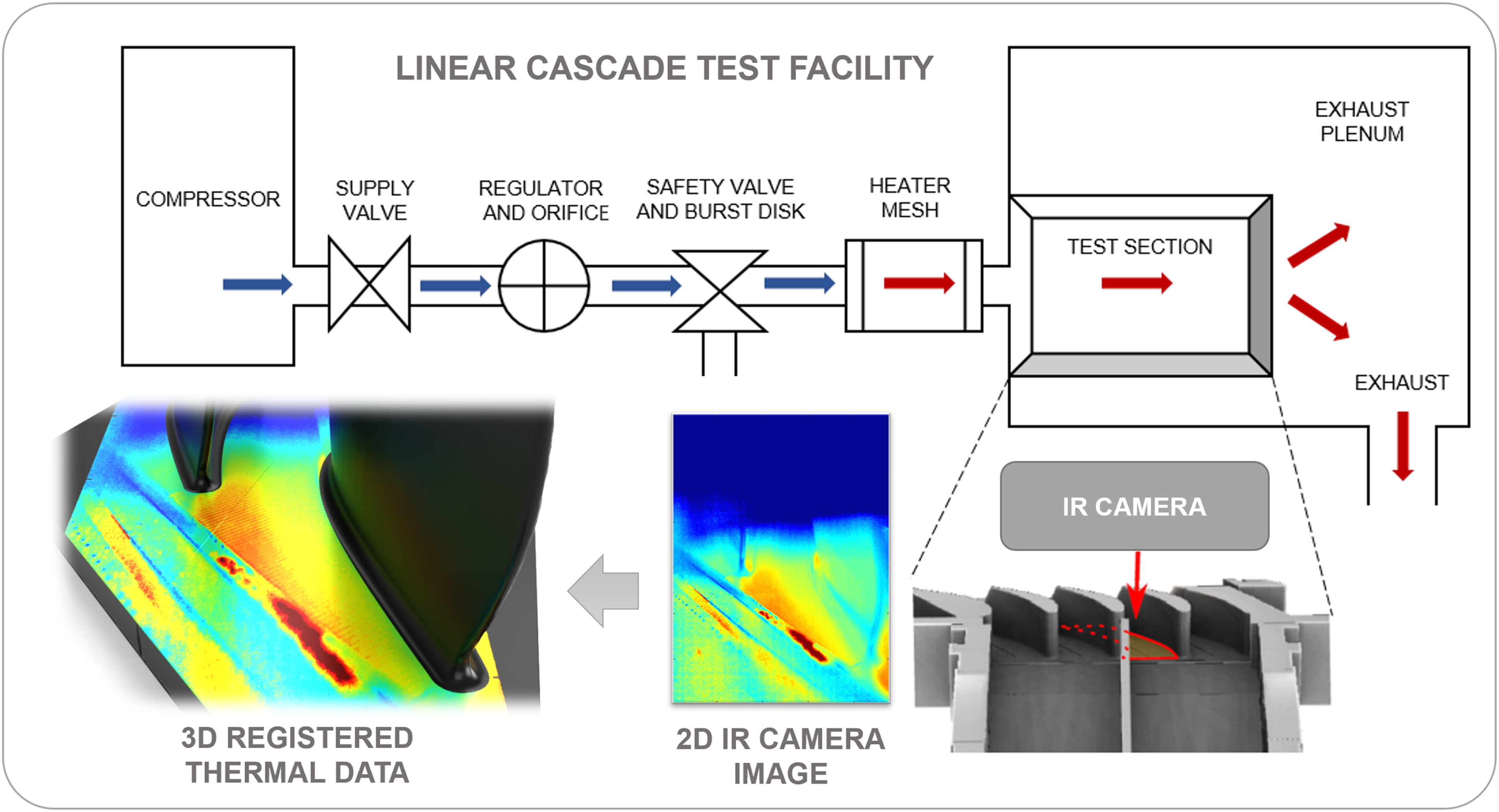
Thermal imaging cameras are increasingly used alongside thin-film gauges as a non-invasive method to measure surface temperature in an experimental environment. Thermography methods offer higher resolution thermal data compared to film gauges but are limited by line of sight access, often obstructed if analysing shrouded components. Methods for calibration and roughness compensation are described by Falsetti et al. (2021), Michaud et al. (2020), and Condren et al. (2023). Many users choose to analyse thermal image data in the native 2D image plane, thus neglecting curvature and other geometric effects. The curvature methods defined in this paper are equally applicable to infra-red data but require that the pixel location and CAD model be aligned, to define the correct curvature at each pixel location. Presented below is a novel 3D thermography registration process that allows these data to be paired, optionally also enabling the data to be applied as a 3D simulation boundary condition.

Traditional IR post-process methods follow the same methodology as thin-film gauges, treating the data pixel-wise and assuming the geometry surface to be planar one-dimensional. The 2D pixel video data is split to a time series of nx×ny 1D temperature data sets then recombined to show a final result. Direct comparison between runs, or with other measurement data, requires the user to manually register the image to account for misalignment. Using computer vision techniques developed by the Oxford Robotics Institute, Hartley and Zisserman (1999), the analysis can be improved by finding the imaging camera matrix described in Figure 11. Knowledge of the CAD model and the perspective projection matrix can be used to automatically register the image to the 3D model. The mapped data is then automatically aligned for run-to-run comparison and can also use the improved non-planar analysis, taking the methods discussed earlier in this paper.

Figure 11.

Definition of the perspective projection thermal camera matrix, P, that maps a real world scene point, S, to the corresponding location on the image plane of the camera, s.

A perspective projection camera is represented by a 3 × 4 matrix, that maps a real-world scene point to it’s corresponding 2D pixel location in the camera image plane. The homogeneous coordinates between two views can be represented by the fundamental matrix P, which combines the camera calibration, rotation and translation matrices. Computing P from a known scene and set of image locations can be reduced to a simple vector minimisation of two equations and labelling a minimum of six known locations in the image.

The homogeneous coordinates are given by normalising the image point, s, following the matrix multiplication of P with S.

These can be rearranged to give linear equations in the matrix elements of P

Then concatenated to generate a 2n×12 matrix, A, such that Ap=0.

This must be solved using the linear least squares solution that minimises |Ap|, taking the smallest eigenvector from the singular value decomposition of A. This is achieved by defining several reference locations, where the global coordinate (X,Y,Z) and corresponding pixel location (x,y) are known.

The resulting minimisation gives the element values of P that best fit the data provided. Accuracy of the fit is important and although the process can be solved with a minimum of six known locations, where possible the maximum number of reference coordinates should be defined by the user to accurately bind the CAD model and the image. Ideally the known reference points should cover the extremes of the region of interest to prevent skew in the extrapolated areas. Well defined locations, for example cooling hole centres, make for ideal candidates in reference point selection. The best fit components of the vector p allow the full matrix P to be constructed. Mapping from the image plane to the higher order 3D space cannot be achieved via matrix inversion. Therefore, the 3D data must instead be mapped to the image and sampled from the lower order space.

In order to sample the image, a surface point cloud of the 3D model is first extracted. This process is best handled using the same STL file previously used to define the surface curvature. Use of the same file provides consistency between the curvature calculation and camera registration processes. Each STL vertex is first mapped to the image using the matrix P, then paired with the corresponding pixel. The resulting pairing gives a pixel reference for each location on the 3D surface thereby allowing the spatial coordinate, curvature and temperature data to be efficiently linked. Following the point-pixel pairing the user has full knowledge of the 3D coordinate, the principal surface curvature at this location, and the thermal time history from the FLIR video. The heat flux can then be calculated, adjusting for the geometric effects where necessary, using either the modified impulse response or radial Crank-Nicolson methods.

Mapping the thermal data to the CAD has additional benefits beyond pure curvature correction. Multiple cameras can all be mapped to a single 3D model, allowing several data sets to be efficiently merged for full coverage of a vane surface using Blender (Blender Online Community, 2023) or ParaView (Ahrens et al., 2004). Exact camera alignment is not critical, and positional variation between runs can automatically be corrected. Static views can be created in the visualisation software, ensuring a consistent analysis across a test campaign. Section and slice controls offer a higher level of control, better allowing the author to communicate the figure intent. Figure 12 shows a schematic of an aerothermal linear cascade, typically instrumented with thin-film gauges or infra-red thermal cameras. The 3D registration allowed the thermal data to clipped by surface, highlighting the endwall region of interest in the original NGV study by Shaikh (2020).

Figure 12.

Schematic of an aerothermal linear cascade test facility, showing a typical 2D infra-red camera image of the turbine NGV endwall and the resulting 3D mapped thermal data on the CAD geometry.

Summary

Thermal analysis of most engineering components requires the evaluation of curved or freeform geometry. Planar surface assumptions, commonly used to simplify the analysis, lead to significant error in the calculated heat flux. Analytic solutions for a 1D cylindrical system have been investigated and applied in the case of aerothermal analysis of a turbine nozzle guide vane. Point-wise solutions were compared to a full 3D ANSYS numerical simulation, proving the reliability and accuracy of the 1D radial method for thin-film heat transfer gauge post-processing.

A novel Cartesian to Cylindrical impulse response was presented, allowing the upgraded methods from the previous paper to be applied on complex freeform geometry. Additional consideration must be given to the semi-infinite limit in cylindrical applications, with further limits on the impulse response test duration. Therefore, a cylindrical upgrade was also discussed for the multilayer 1D Crank-Nicolson scheme, extending the range of suitability to curvature correction.

The new methods necessitate that the point-wise surface curvature be known. A methodology was presented to assess the curvature of complex freeform surfaces via standard stereolithography files and surface triangulation. An extension for thermography image mapping was also introduced, allowing fast robust transfer of 2D thermal camera data to a known 3D geometry. Combination of these techniques allows for full surface analysis, supplementing the point-wise curvature correction method for thin-film gauges.

The error caused by a 1D planar assumption was as high as 11% in some regions and in excess of 4% across the NGV leading edge. In comparison, the curvature corrected method achieved heat flux calculation accuracy within ±1% across all blade surfaces. When using flexible thin-film heat transfer gauges or surface infra-red thermography, it is essential that the effect of curvature be considered and the errors associated with the 1D planar assumption removed. This paper defines the qualitative assessment of the 1D planar assumption and provides the necessary methods to handle the thermal analysis of complex freeform geometries.

Nomenclature