
Introduction
Continued growth of computational power over the past decades has enabled the successful application of computational fluid dynamics (CFD) in all stages of the aero–engine design cycle. Despite the achieved progress in CFD simulation practice, Reynolds Averaged Navier–Stokes (RANS) simulations still play a crucial role in the CFD enabled design cycle. RANS–based simulations impose a significantly lower computational cost, in terms of memory usage and simulation time. For turbomachinery applications, the typical RANS turbulence models are based on the Boussinesq assumption (Pope, 2011) and additional turbulence transport equations that provide a closure for the computation Reynolds stress. The Spalart–Allmaras model (Spalart and Allmaras, 1992) is an example of a one–equation turbulence transport model often used in the gas turbine community. However, despite the RANS simulations’ computational efficiency using the Spalart–Allmaras model, there are still significant discrepancies between computed results and measured data. This realization leads to the question; is it possible to maintain computational efficiency while increasing simulation accuracy?
Recently, Bayesian analysis (Beck and Katafygiotis, 1998; Bretthorst, 1990) has been proposed to address the question of RANS turbulence model calibration towards increased prediction accuracy without computational efficiency loss (Cheung et al., 2011; Edeling et al., 2014a, b). The Bayesian analysis applied to epistemic uncertainty (Dalbey et al., 2020) of turbulence model parameters defines the calibration framework that enables quantification of the plausibility of the given turbulence model to predict the experimentally observed data. The plausibility in this context is defined through the posterior distribution of parameter values that enables determination of maximum a posteriori (MAP) value. We note that it is possible to analyze the model inadequacy using the Bayesian analysis (Oliver and Moser, 2011), but in this study, we limit our analysis to the epistemic uncertainty of model coefficients. The main idea of epistemic uncertainty quantification in Bayesian analysis is the representation of a random function's lack of knowledge of parameters with an associated prior probability distribution. The introduction of random variables, in the otherwise deterministic model, enables the model calibration through Bayesian inference. It should be noted that the introduction of random variables in the turbulence model is a model of uncertainty that does not change the physical nature of the turbulence model.
Kennedy and O’Hagan (Kennedy and O’Hagan, 2000) have established the principles and taxonomy of the Bayesian method of analysis applied to computer models. In the seminal work Kennedy and O’Hagan establish broad–reaching definitions including parameter uncertainties, model inadequacy, residual variability, parametric variability, observation error, and code uncertainty. In addition to named definitions, Kennedy and O’Hagan establish the principles of Bayesian model calibration that have been used in subsequent calibration works. Oliver and Moser (Oliver and Moser, 2011) used the established definitions and Bayesian model framework to treat the epistemic and model inadequacy of several RANS turbulence models. Related work by Cheung et al. (Cheung et al., 2011) used Bayesian analysis for the calibration of the Spalart–Allmaras turbulence model coefficients, and model inadequacy, to reproduce the turbulent boundary layer profile over the flat plate. A comprehensive review of turbulence model uncertainties is given in Xiao and Cinnella (Xiao and Cinnella, 2018). Recently, de Zordo–Banliat et al. (de Zordo-Banliat et al., 2020) applied Bayesian analysis to compressor cascades to produce a set of calibrated turbulence model parameters with emphasis on the turbulence model inadequacy. Many other researchers have used Bayesian inference (Tagade and Sudhaker, 2009; Yıldızturan, 2012; Guillas et al., 2014; Ray et al., 2014; Xie and Xu, 2019) for the calibration of RANS model parameters with success. It should be noted that while a significant amount of research has shown the potential of Bayesian inference to improve the accuracy of RANS models, most works focused on two–dimensional flows. In this work, we apply Bayesian inference to RANS model parameter calibration for the three–dimensional non-equilibrium flow problem of a compressor cascade with the corner separation (Lang et al., 2019).
Corner separation is one of the key phenomena for predicting compressor performance. Corner flow separation appearance and size of the separated flow region has a significant impact on mass flow, efficiency and stall margin that affects both on- and off-design performance of compressors. Although it is known that high fidelity eddy resolving simulation such DES and LES are reliable tools for accurate off-design flow prediction, the computational cost associated with these methods is unacceptable in the design process. On the other hand, RANS CFD is standard design tool thanks to its numerical robustness and short turn around time. However, RANS simulations are known to have difficulties predicting the non-equilibrium flow phenomena characterizing separated flows. While Spalart-Allmaras model has been successfully used for the prediction in turbomachinery practice, it fails to predict corner separation in compressor cascades if the standard set of model coefficients are used. On the other hand, de Zordo–Banliat et al. (de Zordo-Banliat et al., 2020) demonstrate that improvement of the prediction of compressor cascade flows can be achieved if the Bayesian calibration is used to reproduce the experimental profiles. In this work we demonstrate that the set of coefficients proposed in de Zordo–Banliat et al. are not adequate for the prediction of separated flows. We propose a new set of calibrated coefficients that improve the ability of Spalart-Allmaras model to predict corner flow separation. We also demonstrate that the set of calibrated coefficients proposed in this work retain their predictive capability even when applied to simulations with incidence angles outside of the calibration range, thus demonstrating the predictive capabilities of the proposed calibration set.
Calibration of RANS models is a formidable task mainly due to a number of parameters and associated uncertainties that have to be taken into account in the Bayesian inference approach. For example, the Spalart–Allmaras model has seven adjustable parameters, thus making the parameter seven–dimensional. Each parameter has a prior probability distribution associated with it used in conjunction with the corresponding likelihood function for the posterior distribution. Therefore, the dimension of the posterior distribution associated with the Spalart–Allmaras model is also seven. Since the Bayesian inference requires evaluating the posterior probability function to determine the MAP values of all parameters, the high–dimensional nature of the posterior function presents a computational challenge. Clearly, using the original calculation methods for complex three–dimensional flows is not feasible; a more efficient approach is required. In this work, we use a surrogate model combined with the parameter sensitivity analysis to decrease the cost of the Bayesian calibration of parameter values.
The main idea of reducing the computational cost of Bayesian inference is to replace expensive CFD computation with a surrogate model. One approach utilized in this work is the employment of the generalized polynomial chaos (gPC) (Eldred, 2009; Marzouk and Xiu, 2009) to replace expensive three–dimensional computations with a simple function evaluation (Cheung et al., 2011; Lu et al., 2015). The main idea of the gPC is the creation of the spectral representation of the underlying implicit function (CFD simulation) and its dependence on parameter values through using the prescribed function basis and corresponding amplitudes. In this work, we use the gPC framework to construct the CFD simulation data's surrogate model to remove the computational cost associated with the evaluation of the posterior function.
The paper's organization is as follows: we first introduce the Bayesian framework ideas, followed by a description of the experiment and numerical simulation. We then discuss in detail the surrogate mode construction and calibration of turbulence model parameters. Results of the calibrated turbulence model simulations are presented next, and compared to the experiment data. Finally, we present conclusions and discuss future research direction.
Calibration framework
SA model calibrated parameters were calculated from the posterior distribution obtained using Bayes’ theorem; where prior knowledge and likelihood, computed from those input data are combined.
Calculation of the posterior requires prior knowledge and the likelihood function obtained using experimental data, d, and parameterized model coefficients,
The turbulence model parameters,
The prior distribution quantifies prior knowledge, or belief in the parameter values, prior to consideration of new data. In this study, we assume a uniform prior distribution in order to provide a non-informative prior belief in the parameter values. The likelihood function represents the probability of obtaining the experiment data given the parameters,
Likelihood
Proper construction of the likelihood function has a pivotal role in the calibration process. To account for measurement uncertainty in the likelihood function the experimental data was related to the true data using Equation (3), where
The error is assumed to be a Gaussian random variable with zero mean and prescribed standard deviation,
Furthermore, the true data were related to the model parameters via a forward model,
Thus, the likelihood takes the form shown in Equation (6).
Equation (6) can be expressed in vector form when the experimental data are regarded as a vector:
where N corresponds to number of observations contained within d and
Surrogate model
The surrogate model was constructed using generalized polynomial chaos (gPC). With this approach, a function of random parameters is represented as an infinite sum:
where
where N is the order of the gPC expansion. Note that the time coordinate is dropped in further discussion since the case study under consideration was steady state.
The gPC coefficients were computed using spectral projection:
where
Prior to the calibration, SA model sensitivity to parameter variation was analyzed in order to determine which random parameters were most significant in the surrogate model. The sensitivity for each random parameter was determined by first computing the gPC expansion for all parameters:
where the subscript
where
where n is the number of points in the region of interest. Lastly, a threshold,
The surrogate model was then constructed using Equation (10) and a subset of the full random parameter set:
where
where the dependence of
Case study
The linear compressor cascade recently tested in RWTH Aachen university (Lang et al., 2019) was used in this work to provide the experimental results for both calibration and validation of the calibrated turbulence model. To represent the compressor flow physics as closely as possible, the Reynolds number based on chord length of the experimental setup was set to
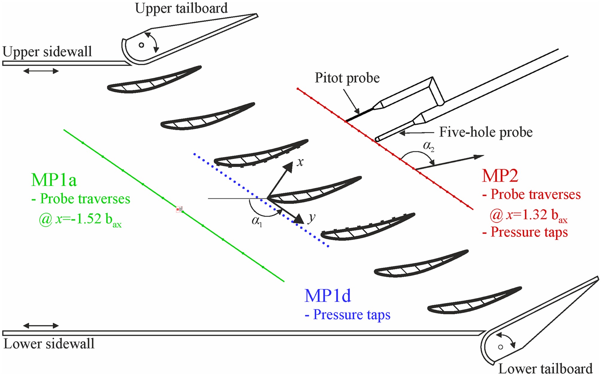
Experimental measurements
Aerodynamic measurements of the flow entering and exiting the cascade row were acquired at
Numerical simulation
Numerical simulations of the Aachen University cascade were executed using UPACS solver (Tani, 2018), developed initially by JAXA (Japan Aerospace Exploration Agency). UPACS is a density-based finite volume solver. For the convection term, the Roe scheme with third order MUSCL interpolation is applied, and second order central difference scheme is used for the viscous term.
Closure of the governing equations was achieved using the Spalart–Allmaras turbulence model (SA). The SA model solves a single transport equation for modified turbulent viscosity, shown in Equation (17), to calculate the eddy viscosity relating turbulent stresses to the mean flow. The calibration parameters were chosen from the set of seven model coefficients in Equation (19).
(18)
Figure 2a shows the computational domain used in this study. To reduce the computational cost of the simulations the upper and lower sidewall effects were assumed to be negligible and the flow through the cascade periodic, therefore only a single pitch was modeled. The ratio of fillet radius to chord length, R/Cx, was 1/15 in the actual geometry and was included in the CFD model. The inlet boundary condition was specified using the experimentally measured total pressure, total temperature, flow angle, and turbulent intensity. The inlet modified turbulent viscosity was estimated from experimental turbulent intensity, turbulent length scale, and mean flow velocity. Radial profiles were specified to account for the endwall boundary layers. A static pressure boundary condition was applied to the outlet of the domain and was adjusted to achieve agreement with the experimental inlet Mach number of 0.7.
Figure 2.
Linear compressor cascade (a) computational domain with the airfoil and hub endwall surfaces shown (other surfaces hidden) and (b) grid around airfoil surface at midspan.
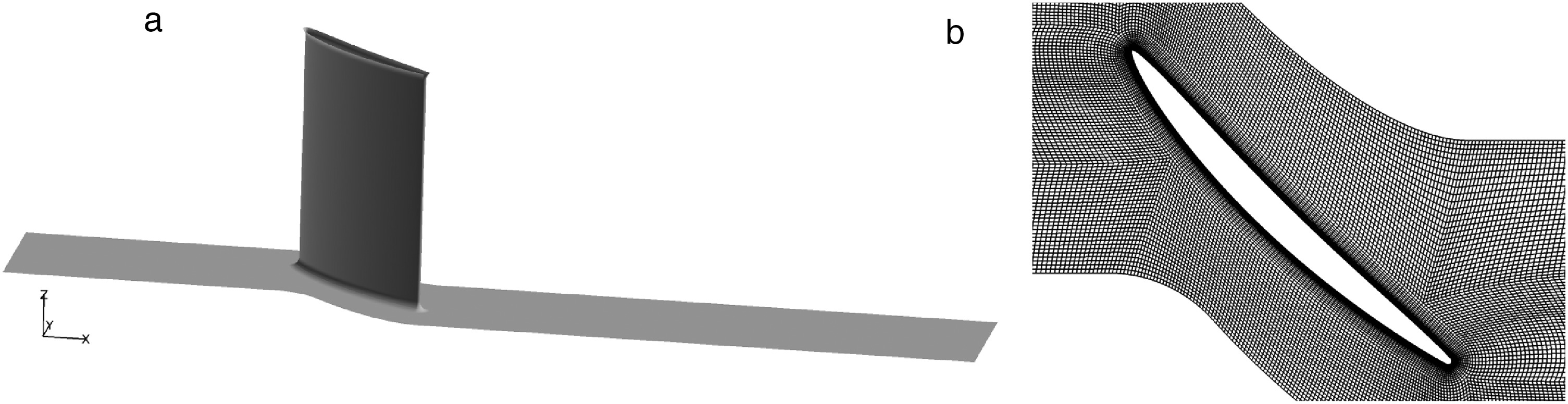
A grid independence study was completed using three computational grids with resolutions of 3.2, 6.8, and 17.3 million cells. Based on area–averaged quantities, a grid independent solution was achieved with a resolution of 6.8 million cells. All simulation results in the following sections were obtained using the 6.8 million cell grid. A cross–sectional view of the airfoil grid is shown in Figure 2b. The spanwise direction consisted of 188 points with higher density near the endwalls. The airfoil and endwall boundary layer meshes were constructed to have a first cell height of
Surrogate model construction
Seven turbulence model parameters were considered for calibration in this study:
it was readily available from the experimental data set,
it was nondimensional, and
it clearly showed evidence of the corner flow separation.
Prior to constructing the surrogate model, a sensitivity analysis was done to determine the most influential parameters of the set. Less influential parameters were then discarded from the calibration set in order to reduce computational cost while maintaining sufficient accuracy for the model calibration. The sensitivity analysis was done by computing a 1st–order gPC expansion for each parameter. This choice was motivated by the low computational cost and provided sufficient accuracy to quickly narrow down the most important parameters. Note that the chosen accuracy would have been reconsidered if the calibration had yielded unsatisfactory results. The parameters were assumed to be uniformly distributed on the interval
The model evaluations are shown in Figure 3a. The curves correspond to the expected value of Mach magnitude at 90% span in the downstream measurement plane, which is a region of interest due to the corner separation. The vertical bars represent
Figure 3.
Sensitivity analysis in downstream wake region: (a) Wake profiles at all quadrature points and (b) Sensitivities for all seven parameters considered.

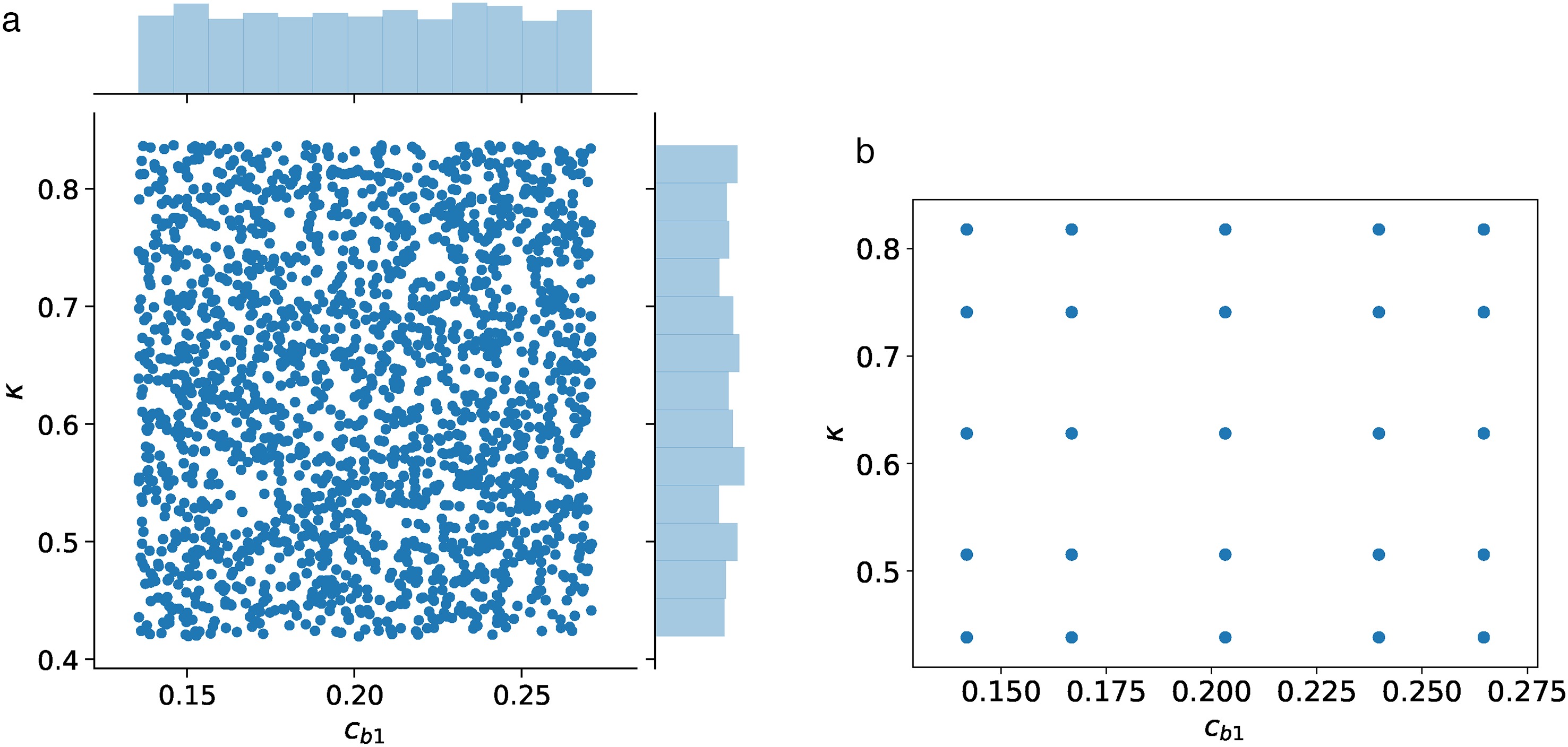
The surrogate model of Equation (15) was constructed using a 4th–order gPC expansion and the parameter set
Figure 4.
Prior assumption and corresponding nodes for c b 1 κ
The model was evaluated at the 25 quadrature nodes and the gPC expansion was constructed for the Mach magnitude. The expected value of Mach magnitude is compared with experiment data in Figure 5. Both data sets correspond to 90% span in the downstream measurement plane and are sampled on the same pitchwise coordinates. Note that the data sets were shifted to match the location of minimum Mach number because no reference position was available from the experiment data. The vertical bars on the expected value curve represent

Parameter calibration
Mach magnitude was chosen as the parameter of interest for the reasons provided in the previous section. The calibration data set was then chosen to be the experiment Mach magnitude profile at 90% span in the downstream measurement plane. This location was chosen specifically for its direct correspondence with the corner separation. Furthermore, this selection also demonstrated the calibration method's effectiveness even when using a limited data set. For example, later we compare the calibrated model's total pressure prediction with experiment.
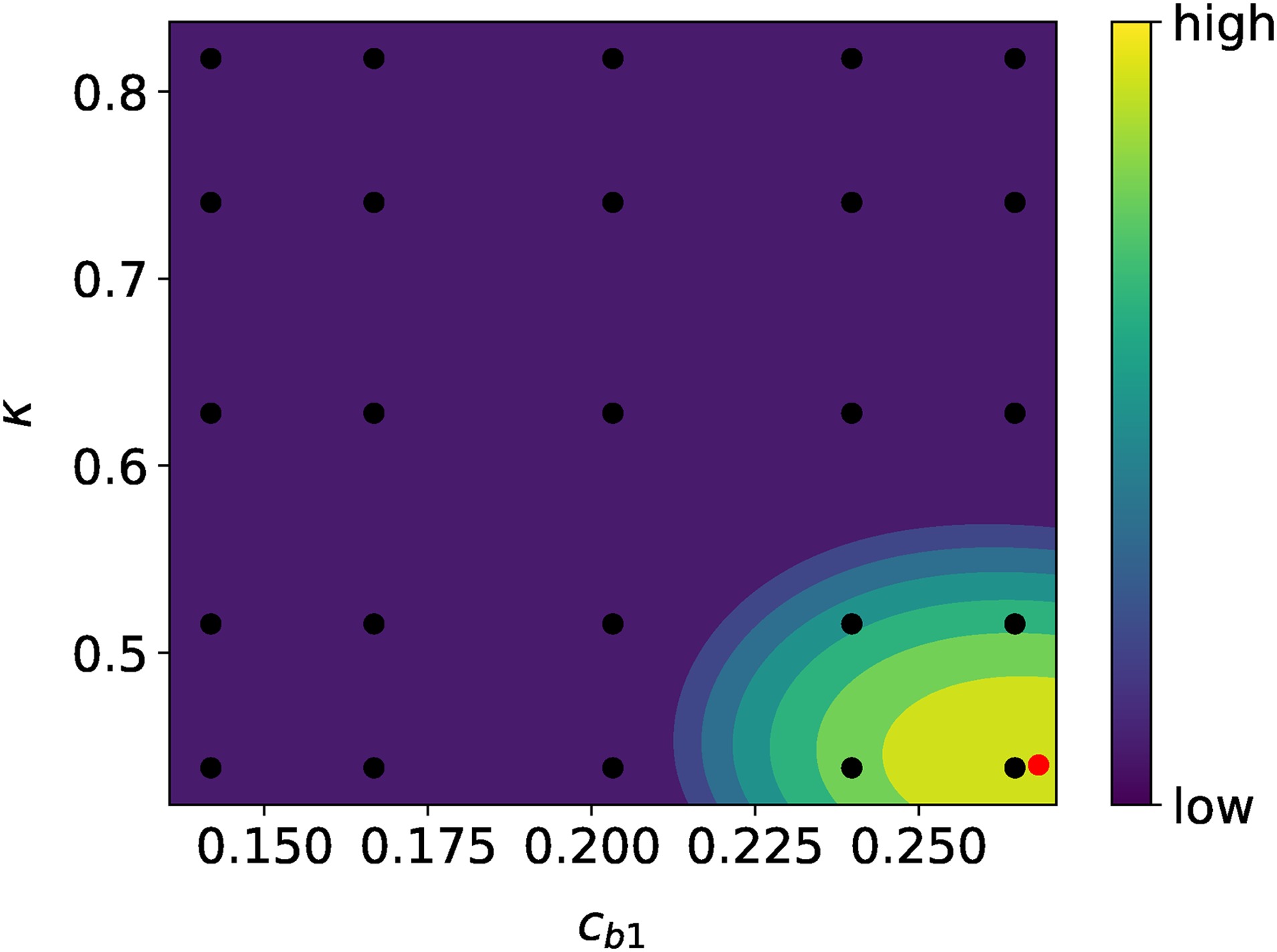
Figure 6 shows components of the calibration process.The gPC surrogate model was constructed for Mach magnitude at each point of the profile. An example response surface from the gPC surrogate model is shown in Figure 6a. The probability density function (pdf) computed from gPC was compared with the experiment data pdf which was prescribed by Equations (3) and (4). The likelihood function quantifies the probability of the obtaining the experiment data given the model parameters but is interpreted as a function of the model parameters. An example likelihood is shown in Figure 6c for a given experiment data point.
Figure 6.
A single point calibration process: (a) gPC response surface, (b) experimental data and gPC surrogate model output, and (c) likelihood.

The posterior at each data point was constructed according the Bayes’ Theorem (Equation 1). The final posterior was then defined as the product of all posteriors, i.e.:
where
Calibrated result
Calibrated parameter values larger than nominal, for both
The following include results for three SA model parameter sets: (1) parameter values calibrated using Bayesian inference approach defined in the current study (“calibrated”), (2) nominal SA model parameters (“default”), and (3) scenario 2 parameter values reported by de Zordo-Banliat et al. (2020) (“reference”). First, the effect of the calibrated parameters on the numerical result are described. Next, the calibrated model is compared to experiment data, the “default” result, and the “reference” result at the design condition. Lastly, the predictive capability of the calibrated model was assessed and compared to the previously mentioned data sets at off–design incidence angles.
Influence of parameter calibration
Calibration of the SA model parameters
Figure 8.
Turbulent viscosity normalized by molecular viscosity at MP2 for numerical solutions using (a) calibrated SA model parameters and (b) default model parameters.
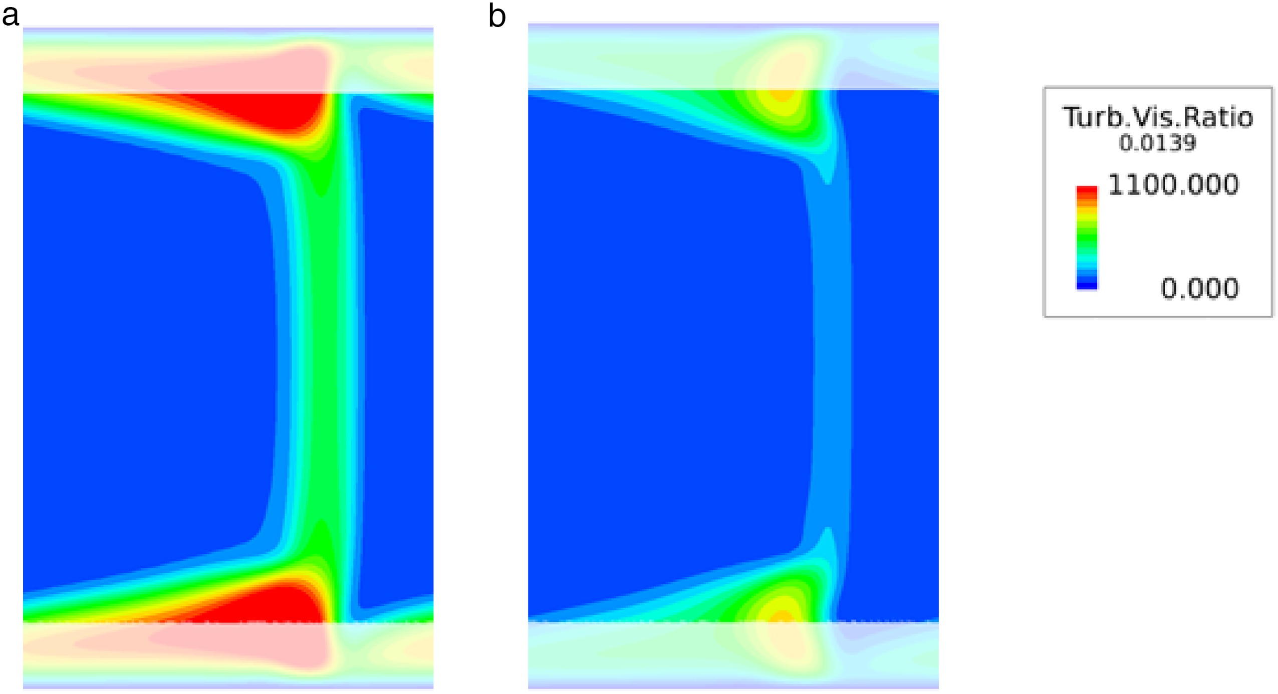
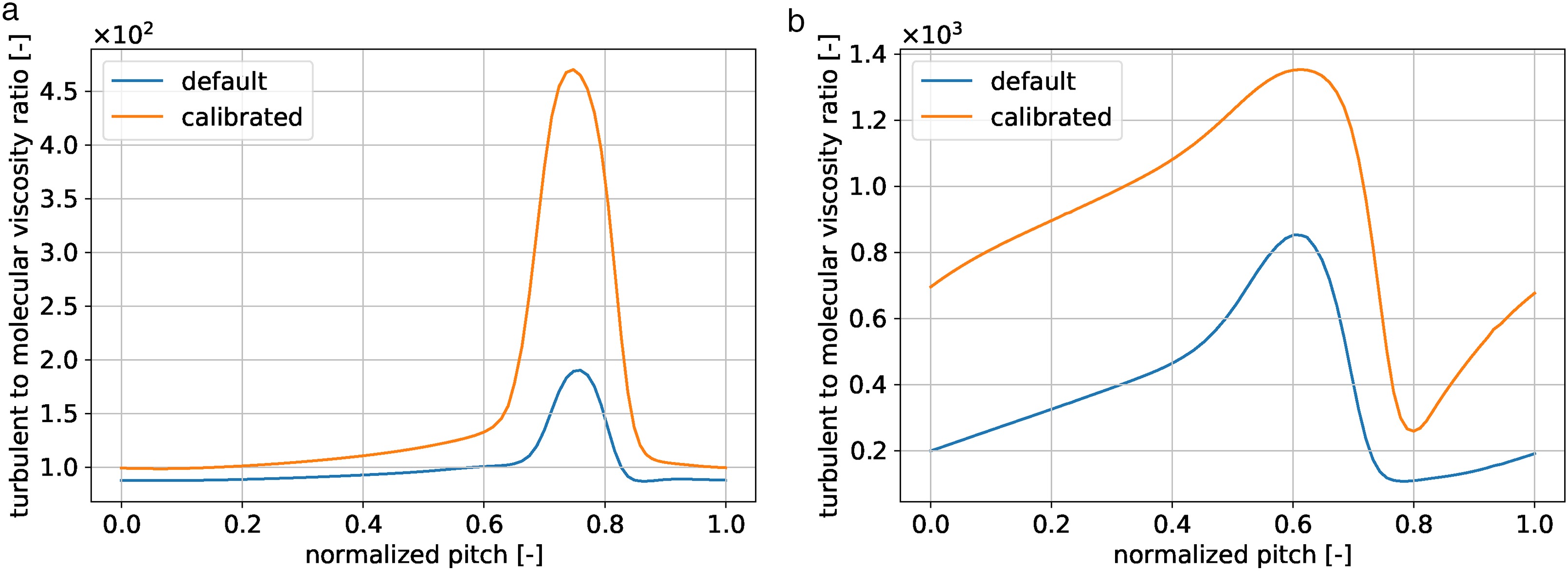
Figure 9.
MP2 profiles of the wake turbulent viscosity normalized by molecular viscosity in the pitchwise direction at (a) 50% and (b) 90% span.
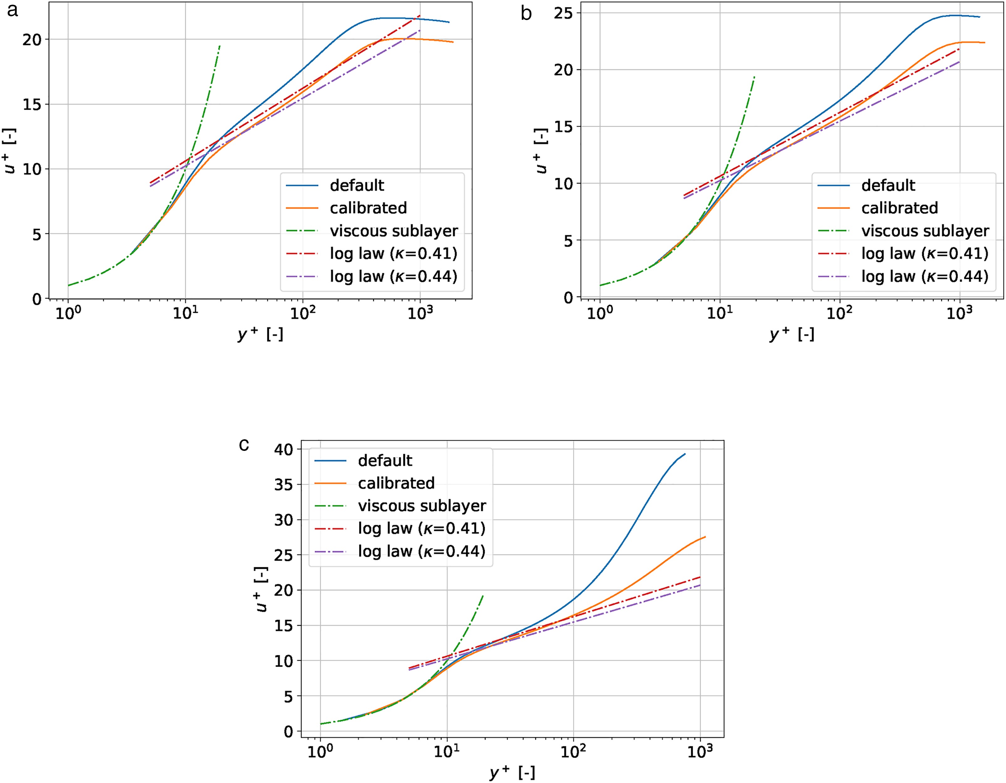
Equation (21) shows the theoretical form of the log layer velocity profile. Here,
Figure 10.
Comparison of dimensionless streamwise velocity ( u + ) ( y + ) κ = 0.41 κ = 0.44
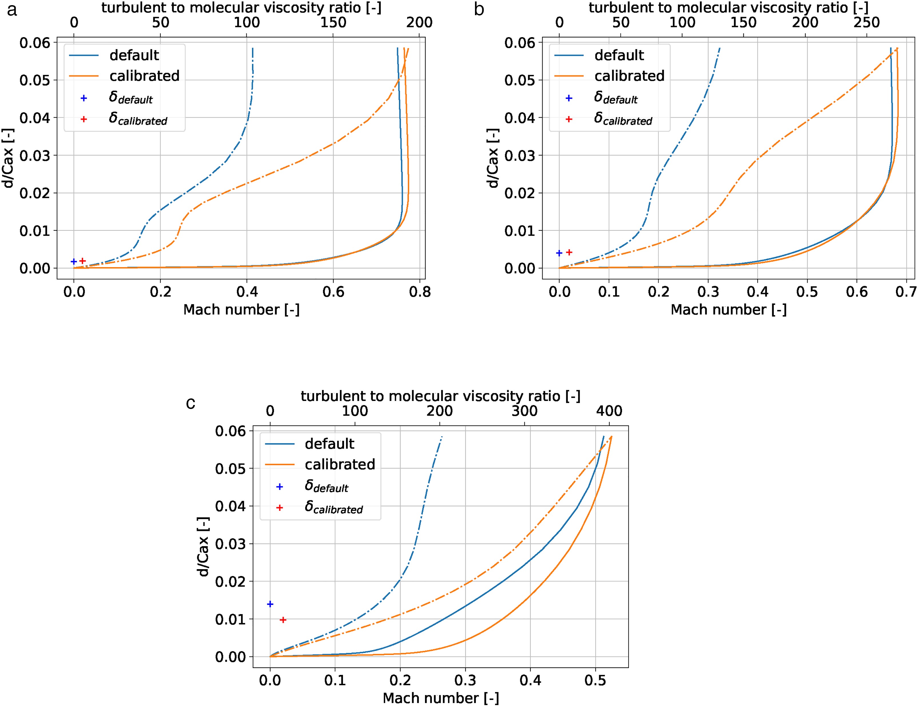
Wall-normal profiles of Mach number and turbulent viscosity are also shown in Figure 11. In addition, the “calibrated” and “default” boundary layer displacement thicknesses are plotted near the vertical axis. At 20% and 50% axial chord, the “calibrated” boundary layer thickness is shown to be consistent with the “default” results. However, at 80% chord the “calibrated” results show a increase in the turbulent viscosity growth and decrease in the boundary layer thickness. This result coincides with the reduction in corner separation area that will be discussed further in the next section.
Figure 11.
Airfoil wall-normal profiles of Mach Number (solid line) and Turbulent Viscosity normalized by molecular viscosity (dashed line) at 90% span and axial locations of (a) 20% Cx, (b) 50% Cx, and (c) 80% Cx from simulations using default and calibrated model parameters. Displacement thickness (+) is plotted for reference.
The 50% span blade loading and wake Mach number profiles are shown in Figure 12 to assess the overall impact of changes to the modeled turbulence observed in the boundary layer and cascade, resulting from the parameter calibration. The horizontal axis is normalized chord and the vertical axis is blade Mach number. The “calibrated” midspan loading result in Figure 12a shows the flow accelerating over the suction side, near the airfoil leading edge and reduced error with respect to experimental measurements. This coincides with the improved prediction of corner separation, resulting blockage, and incidence change effects of the parameter calibration. The remaining disagreement between experimental data and “calibrated” results was associated with measurement uncertainty, geometric/periodicity error, two parameter limited calibration, and choice of experimental data used in the calibration framework.
Figure 12.
Comparison of (a) cascade airfoil loading Mach magnitude profile for measurements (exp.), simulation using calibrated model parameters (calibrated) and simulation using default model parameters (default) and (b) wake Mach magnitude profile for measurements (exp.), simulation using calibrated model parameters (calibrated), simulation using default model parameters (default), and simulation using reference model parameters (ref.)
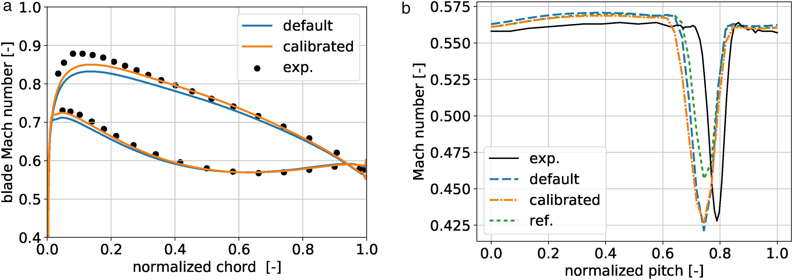
Figure 12b shows that both parameter sets (“calibrated” and “default”) predict an offset peak wake deficit with respect to measurements. The “reference” results were observed to under predict the wake deficit while the “calibrated” and “default” simulations show good agreement with experimental data. All three parameter sets over-predict the recovery Mach number outside of the suction side wake (lower values of normalized pitch). The results in Figure 12 showed marginal, yet positive, solution influence outside of the corner separation region. Further optimization to include the mid-span region may be possible by including more experimental data into the calibration data set. Since the calibration is focused primarily on improving prediction of corner separation, further optimization was deemed unnecessary.
Prediction of corner separation
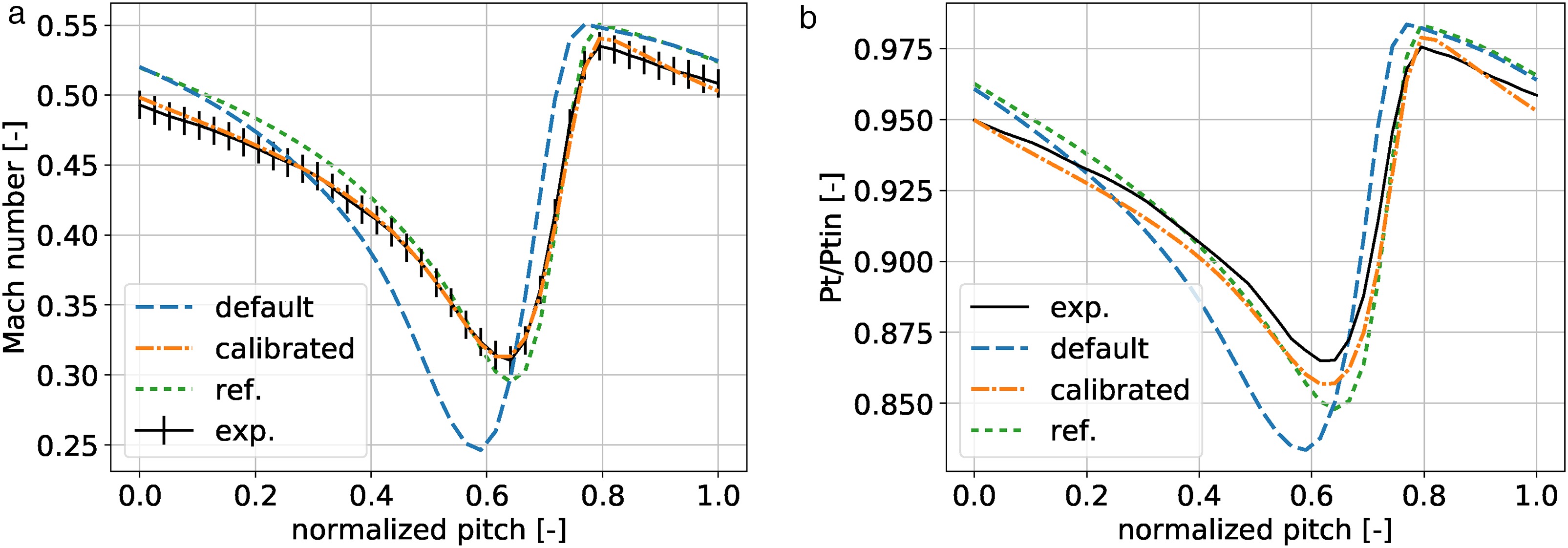
Results in this section are focused on the effectiveness of the calibration to improve prediction of corner separation at the design condition. Figure 13 shows a comparison of the measured Mach number distribution at MP2 with the “calibrated” and “default” results. The general wake structure obtained from both “calibrated” and “default” simulation results show a qualitative agreement with experimental measurements. However, the “calibrated” results show a decrease in the spanwise and pitchwise extent of the secondary flow effects in the corner separation region when compared to the “default” results. This effect is highlighted in the 90% span pitchwise profiles, shown in Figure 14. The parameter calibration is shown to reduce the numerical error, with respect to measurements, in the prediction of corner separation wake Mach number (Figure 14a) and total–to–total pressure ratio (Figure 14b) compared to the “default” result. Additionally, in comparison to the “reference” results, the “calibrated” simulation shows improvements in predictive capability across the passage width. This result shows the effectiveness of the parameter calibration to reduce over–prediction of the corner separation losses and flatten the wake profiles in areas of the flow where both “default” and “reference” results fail.
Figure 13.
Two-dimensional wake Mach number distribution at MP2: (a) experimental data, (b) calibrated CFD and (c) default CFD.

Figure 14.
Pitchwise (a) Mach number and (b) total-to-total pressure ratio profiles obtained from measurement (exp.), simulation using default model parameters (default), simulation using calibrated model parameters (calibrated), and simulation using reference calibrated model parameters (ref.) at 90% span.
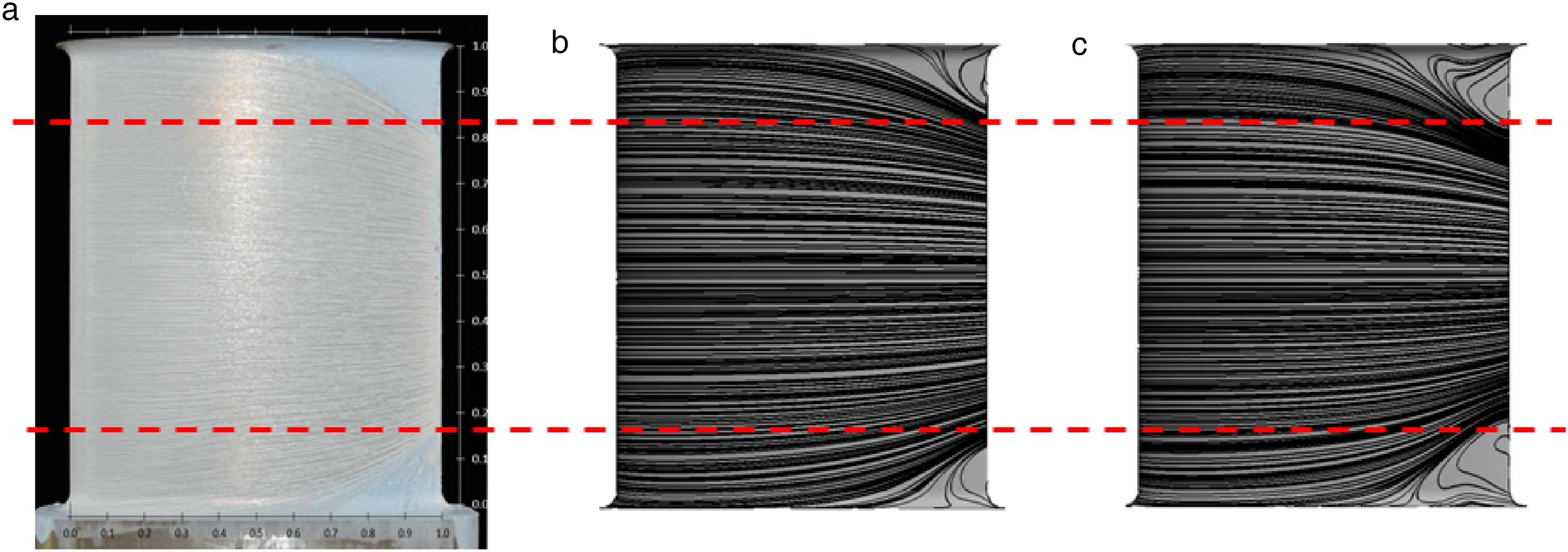
The combination of the aforementioned results have shown that turbulence model parameter calibration via Bayesian inference is a capable of improving the prediction of corner separation. Surface flow visualization, shown in Figure 15, clearly shows that the calibrated CFD reduces the over predicted size of the separation region computed using default turbulence model parameters. In addition the calibrated results are qualitatively in agreement with the experimentally measured corner separation area, indicated by dotted lines.
Off-design application
The predictive capability of the calibrated model was assessed by comparing the calibrated result to experiment at off–design incidence angle. Experiment measurements of Mach magnitude in the downstream measurement plane (MP2) were available for the following off–design incidence angles:
Figure 16.
MP2 Mach number with respect to normalized pitch at 90% span for varying inlet flow incidence angles of (a) − 5 ∘ − 3 ∘ + 3 ∘ + 5 ∘
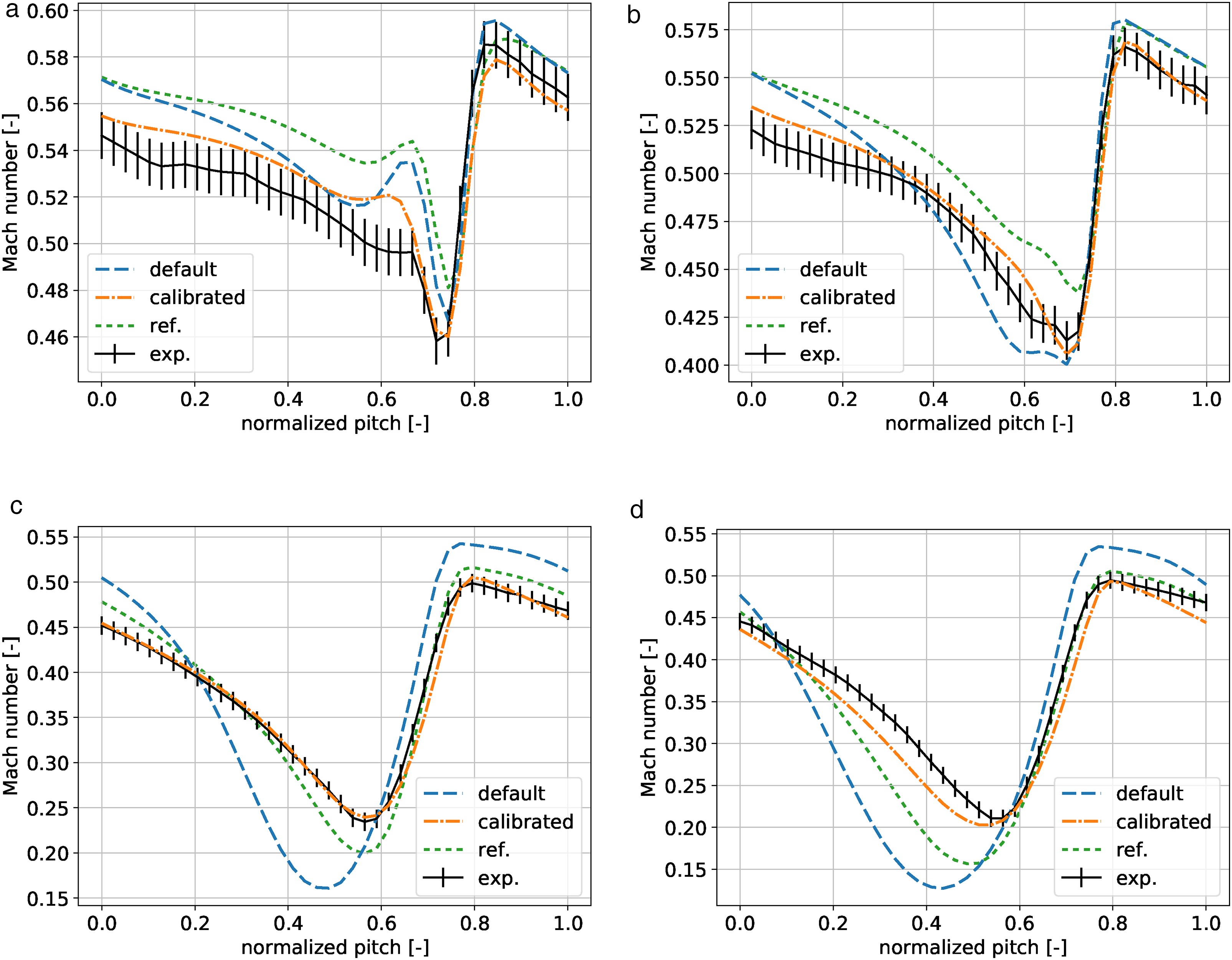
The influence of the corner separation increased with increasing incidence angle. This was observed in the decreasing minimum Mach number, e.g. 0.31, 0.24, and 0.21 for
Conclusion
Bayesian inference was used to calibrate RANS turbulence model parameters and improve flow prediction in a linear compressor cascade. The Bayesian calibration framework was developed and construction of the likelihood function was shown. A surrogate model was also constructed via generalized polynomial chaos (gPC) in order to reduce computational cost. Sensitivity analysis was used to reduce the parameter set and further decrease computational cost while maintaining sufficient accuracy. The posterior probability distribution was computed and the calibrated parameters were determined from the maximum a posteriori (MAP) value.
The calibration framework was applied on corner separation in a linear compressor cascade. Previous experiments provided the data set used for calibration. The numerical model was 3D steady state RANS and used the Spalart-Allmaras turbulence model. The quantity of interest (QOI) for calibration was Mach magnitude at 90% span in the downstream measurement plane. This location was chosen because it lies within the region where the corner separation is predominant. The random parameter set consisted of
The calibrated CFD model was compared to CFD with default parameters and experimental data. The calibrated model showed accurate prediction of the corner separation and the pitchwise wake profile. This improvement was associated with enlarged turbulent viscosity, which resulted from increased turbulent production by modified
This study showed successful calibration of the Spalart–Allmaras turbulence model for a corner separated flow in a linear cascade. The calibrated CFD will be carefully introduced into the design process with the goal of improving prediction capability. This calibration only focused on two parameters, one geometry, and one region of the flow. Further investigation of the other model parameters and other flow features will be continued.