
Introduction
Failures of engineering systems can cause catastrophic consequences such as loss of lives, environment contamination and huge financial costs (Rasmussen and Rouse, 2013). In energy production applications, achieving high reliability and availability is a crucial task which requires adoption of efficient maintenance policies. Turbomachinery and production plant complexity, in addition to limited data availability, have restricted in the past the capability to predict functional anomalies and component degradation phenomena that can lead to failures or may cause unnecessary maintenance interventions with consequent system unavailability. The lack of modelling capabilities combined with the need to mitigate risk of failure, led the adoption of preventive maintenance strategy (maintenance is performed at predefined time intervals) where engine is stopped and inspected frequently in order to monitor components degradation phenomena. This preventive strategy impacts on maintenance and environmental cost because parts still serviceable are scrapped and the risk of catastrophic unpredicted failures remains high.
Nowadays, the availability of big data from online monitoring and advanced inspection technologies has opened the era of digital twins, intended as asset virtual replica that can be trained to detect degradation phenomena, functional anomalies, and forecast them over the future to estimate the residual useful life (RUL) and establish the optimal time to maintenance. Digital twin developed by Baker Hughes is an analytics framework combining physics-based and data-driven models that describe the functional and health status of asset components and systems, modelling also their mutual interaction and the overall impact on engine performances (Carlevaro et al., 2018).
The availability of asset digital twin promotes a prescriptive approach where the anomalies are detected in early advance and their behavior is forecasted over the future to estimate time to failure. A decision layer, based on risk-assessment, is then used to suggest corrective and risk mitigation actions to be executed on the asset by maintenance operators. This approach focuses on predictive maintenance, investigated in the last decade as a more effective and proactive maintenance strategy. Its general idea is to predict the future evolution of the systems health status and to take decisions accordingly (Mobley, 2002). Several efforts have been conducted in the recent years to apply Machine Learning to diagnostics and prognostics of turbomachinery assets, leveraging on the availability of online monitoring data (Liu et al., 2018; Manikandan and Duraivelu, 2020). Prognostics and Health Management analytics are widely applied in industry to early detect signal anomalies, assess the health status of the asset and predict its future behaviour. Prognostics is becoming the pillar of maintenance optimization services, but it can’t be considered a synonym of predictive maintenance. Prognostics refers to the capability to early detect an anomaly and establish how the anomaly will evolve in the future. It is able to predict each single anomaly or failure mode and it doesn’t require to describe the interaction between the failure modes and their impact in reducing the asset expected performances or residual life. For example a prognostics algorithm can alert about the risk of an upcoming system failure and estimate when the failure will occur but it is not required to suggest which corrective action has to be taken and which will be the impact of the failure on the overall health status and the expected residual life of the engine. Predictive maintenance is a wider concept that requires the availability of prognostics analytics, in addition to the capability to model the interactions between the failure modes and to optimize maintenance timeline and scope of work (Van Horenbeek and Pintelon, 2013). Effective predictive maintenance combines prognostics with a deep knowledge of functional asset model and a risk-based maintenance policy.
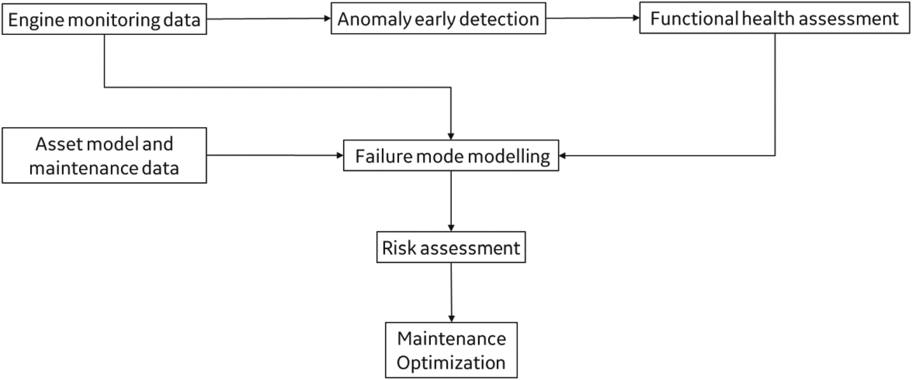
The development of a predictive maintenance framework requires a decision process in place, linking asset online monitoring to maintenance execution (Jardine et al., 2006). The schema starts from early detection of anomalies performed on live operational data, it continues with failure mode identification and modelling, ending with estimation of risk of asset failure and optimization of maintenance scope of work and timeline (Figure 1).

Methodology
Decision support process for maintenance optimization
The predictive maintenance method proposed in this paper consists of a decision support process that, leveraging on data, analytics and domain knowledge, feeds a prescriptive framework providing operation and maintenance insights. The decision flow relies on a data processing path that identifies functional anomalies and evaluates the probability that they will cause a failure of the asset itself or its subsystems. Risk estimation is then obtained weighting the probability of the failure by its impact on asset serviceability and maintenance, evaluated in terms of time and cost needed for asset refurbishment, and consequences on health and safety of people and environment. A correct planning of turbomachinery maintenance has to be performed several months in advance, requiring analytics to model asset behaviour, identify the failure modes and predict damage growth within the expected asset life-cycle (Zio, 2012). Prediction accuracy is a differentiator in prognostics applied to assets with very long life and continuous operation requirements. The complexity relies on the fact that engine-to-engine variability depends both on operational parameters but also on specific conditions like engine assembly and maintenance activities executed offline. The proposed solution is to minimize uncertainty and to control model complexity by combining data-driven modelling with physics-based constraints in order to improve prognostics capabilities and to achieve the expected accuracy, needed to switch from preventive to predictive maintenance.
The merge of data-driven analytics with physics-based modelling is the area of Physics-informed Machine Learning, embracing a wide range of methodologies linked by the capability to balance data-driven and physics-based approaches on the basis of available data and domain knowledge. The modelling can leverage on the availability of big data, represented by live and historical sensors acquisitions and data collected during maintenance and inspections, like measurements taken on defects and failure modes, pictures of damages and reports detailing maintenance activities executed. The data-driven approach is limited only by the availability of data and it is strongly used in prognostics for anomaly detection on live monitoring data. The prediction accuracy is usually limited in time, making the data-driven approach strongly used for fast events prognostics while for long time predictions, the poor capability to extrapolate governing equations, leads to uncertainty propagation of sensors noise within the prediction model. Furthermore, the capability to monitor by sensors the critical failure modes is limited because several engine components operate in harsh environment, like high speed and temperature, with no sensors close to the most critical parts. In addition, the complexity of engine assembly requires to model not only the single failure mode but also the mutual interactions of degradation phenomena and their combined effect on the asset reliability. To overcome the weaknesses of purely data-driven methodologies, turbomachinery domain knowledge is injected within the predictive maintenance analytics framework to achieve more accuracy and to model governing equations of asset functional and health behaviour. The hybrid approach is applied both for the development of each single analytic but also to manage and sustain the decision process, where the anomaly detection is leveraging for the majority on live data while failure mode identification, risk assessment and maintenance optimization steps are strongly driven by turbomachinery domain knowledge and experience.
The decision process starts identifying failure modes and their severity, consequently driving risk assessment and time to maintenance estimation. The failure mode assessment distinguishes between functional anomalies related to engine subsystems malfunctioning and aging/degradation phenomena impacting single components. These two paths of analysis can be linked in a single flow, when component degradation is resulting in a system malfunction, or they can be independent phenomena, when degradation is not impacting the functional status of the asset and it remains undetected till the final failure. The decision process ends with maintenance optimization step execution that, analysing risk trend and estimated time to failure, establishes the proper maintenance action plan to mitigate the risk of failure and to restore the engine functional health status (Figure 2).
Functional health assessment
Functional health assessment is the foundational layer of predictive maintenance, considering that maintenance goal is to restore assets functional health status and expected performances. The functional assessment path is to identify anomalies on acquired and calculated operational parameters, classify them and identify impacted system, distinguishing functional anomalies from sensors fault signatures. The importance of differentiating system functional issues from sensors anomalies is justified by the accuracy requirements that need incorrect readings removed or corrected before the measurements to be processed by the subsequent failure mode identification layer.
The availability of asset monitoring data and fleet experience allows to perform health functional assessment by taking advantage of a wide set of data-driven methodologies that ensure anomalies are identified at early stage and prognostics are applied. The injection of domain knowledge consists on calculated parameters added to input dataset, like asset performances and fleet baselines calculation and the knowledge-based map between anomaly signature and the specific sensor or system issue. The overall health assessment model is then, again, an example of hybrid approach combining data-driven analytics with physics-based modelling (Michelassi et al., 2018).
An example of health assessment methodologies applied within predictive maintenance framework is here following described. It performs early anomaly detection using Auto-Associative Kernel Regression (AAKR) signal reconstruction and a subsequent anomalies classification (Baraldi 2015a). AAKR is applied to reconstruct continuously a reference set of healthy statistical features and to compare them with the same statistical features extracted from acquired or calculated timeseries. Basing on the value of a chosen distance metric, the statistical signature is recognized as anomalous or healthy. In case of anomaly is detected, a subsequent classifier assigns the most likely anomaly category selected from a reference library build on fleet experience. Finally, a knowledge-based logical network differentiates from anomalies related to system malfunctioning or to sensor fault.
The procedure consists of the following steps:
Signal pre-processing: the signals are filtered based on some signal-dependent rule (e.g., during steady-state or transient operation depending on shaft speed).
Training and validation set selection: we choose a large enough number of signal samples in healthy condition, which constitutes the reference for the normal condition. We rely on the assumption that a signal of a gas turbine belonging to a homogenous fleet is in normal condition if its statistical distribution is close to that of the same signal of the other gas turbines in the fleet at the same time instants. We select the signal of the gas turbines which has the minimum average Wasserstein distance (Rüschendorf, 1985) from the others. For each signal s, a collection of measurements
Feature extraction: for each signal, we extract F statistical features (e.g., standard deviation, kurtosis, skewness) on a chosen time window of length W. This entails that the available measurements are divided in groups (batches) of
Feature reconstruction: we reconstruct the value
where the weightsAnomaly detection based on residual. The deviation (residual) of the feature vector between the signal reconstruction and the observation is compared with a properly defined threshold d.
If
Anomaly injection on training and validation set. We consider a selected set of common anomalies which affect sensor measurements (spikes, step changes, freezing, noise,…) and inject these anomalies on each batch of signals extracted from
Anomaly classification based on logistic regression. We train an algorithm based on logistic regression with lasso penalization (Johnson and Wichern, 2002; Zou and Hastie, 2005) on the features extracted from the injected anomalies. The hyper-parameter of the lasso penalization value is selected according to 5-fold cross-validation and the accuracy of the algorithm is tested on the features extracted from the validation set. The anomaly classification algorithm is tested on the feature vector
Anomaly severity assessment. We applied a knowledge-based rule to assign the severity to each anomaly class, identifying the system or sensor affected by the anomaly. Each anomaly class is assigned to the system or sensor which refers to, using a mapping network based on experience and domain knowledge. For example, a step change in a specific signal pressure is identified as an effect of flow seals damage, while a freezing signature is assigned to a sensor issue. The characteristic of the anomaly signature, like persistence and hysteresis, are used to evaluate the severity of each issue.
Hybrid modelling of risk of failure
Risk assessment process starts from failure mode analysis, performed to identify causes and effects of functional anomalies detected on signals and to assess aging and degradation phenomena of components and materials. Failure mode identification can be performed through direct detection by sensors or indirect modelling by analytics. Issues resulting in signal anomalies can be detected through data analytics; other aging phenomena, related to component and material distress, are not producing functional anomalies in the early stage and they need to be monitored through dedicated prediction models able to indirectly estimate damage accumulation by processing acquired and calculated operational timeseries. In case system or sensor functional anomalies are detected, the failure mode assessment is executed by analytics exploring which is the issue most likely related to the detected anomaly signature, allowing the data processing path to link anomaly detection to failure mode analysis and risk assessment. (Allegorico and Mantini, 2014; Iannitelli et al., 2018).
Failure mode modelling
Critical failure modes are modelled using engine operational and maintenance historical data. The choice of modelling approach depends on problem complexity, availability of data and knowledge on failure modes. When a large amount of data is available, the data-driven approach is enough to enable prognostics and predictive maintenance capabilities, being the only choice also when physics of failure mode is unknown. The weaknesses of purely data-driven approach are that the resulting transfer functions are not usually interpretable and prediction accuracy is poor for long time forecasts. Furthermore, if operational data are always available, maintenance data have limited coverage because collected only at end of life or at inspection intervals. The result is an unbalance between input and output datasets, represented respectively by operational data and damage measures collected at maintenance. The model is then not well constrained and the solution is underdetermined (Brunton and Kutz, 2019). Another weakness of the pure data-driven approach is that is not capable to model the interaction of different failure modes contributing to the overall degradation status observed at inspections. When the complexity of the phenomenon is limited and domain knowledge is available, a hybrid modelling approach can be proposed to combine physics-based and data-driven techniques. Accuracy improvement is guaranteed using physics-based models capable to generalize governing equations applied to simulate different future scenarios of engine operation and the related impact on risk of failure. The capability to model the engine degradation in a what-if scenario, opens the possibility to predict time to failure and optimize operation and maintenance, extending engine residual life with expected reliability and performances.
The most challenging case is when the governing equations are not known or too complex to be modelled, acquired signals are poorly informative of the failure mode growth and the damage measures are taken only during inspections performed at major maintenances. In this case the failure mode growth can be modelled only through a data-driven transfer function between engine operational parameters and failure mode measures collected at inspection. Injection of domain knowledge and physics is used outside the failure mode modelling, to perform calculation of relevant features increasing information content of input dataset. We summarize here following the modelling steps of an example of hybrid approach with data-driven modelling combined with physics-based features engineering. The test case presented is a creep deformation phenomenon where high temperatures and pressures cause deformation of turbine hot gas path seals that can lead to final contact between rotating buckets and stator assembly.
Label significance analysis. The description of the failure mode is available through measurements taken at major maintenance intervals (tens thousands of hours) reporting amount of damage accumulation and the overall severity. The available labels are then numerical features representing the measures of the damage, in addition to categorical features representing the overall severity. Significance analysis allows to select the labels that are coherent and that better describe the damage growth range. In the test case considered, the available labels are the numerical residual gap between bucket and stator assembly and the categorical creep severity.
Physics-informed features engineering.
Data augmentation. Domain knowledge of asset functional modelling and root cause analysis are applied to identify which are the features driving failure mode initiation and growth. The identified parameters are not always available among the acquired measurements and must be estimated through physics-based modelling or data analytics (Pawełczyk et al., 2019).
Features transformation. The difference of data type between input dataset (continuous time measurements) and labels (discrete time samples) must be addressed with proper data pre-processing before proceeding with failure mode modelling. In particular, the intent is to transform input timeseries in aggregated features able to describe the overall history of the component life, meaning to translate the historical trend of each measurement in a single value representative of the entire maintenance-cycle. The aggregated parameters obtained from timeseries transformation can be then correlated with failure mode attributes, like accumulated damage and severity. The aggregation of timeseries can be performed by extracting statistics from the historical trend, calculating counters like number of events or number of samples within a certain parameter range, or obtaining some energy related parameter by multiplying extracted statistics with counters. The result is having homogeneous input and output datasets, dealing with parameters that are representative of the same timeframe.
Features selection. With the processed and homogenous dataset composed by features and labels, the selection of relevant inputs can be performed applying suitable comparison metrics. The goal is to find which is the optimum set of input features that explain the relevant information needed to predict output labels. The choice of the metric used to select features depends on data type. In the presented test case, we combined correlation metrics and mutual information to select the best input features to estimate available numerical and categorical labels. The applied correlation metrics are Pearson’s, Spearman’s and Kendall’s correlation coefficients (Chok, 2010).
Pearson’s correlation is a measure of linear relationship between numerical variables
where n is the number of samples.Spearman’s correlation is equivalent to Pearson’s correlation calculated on variable ranks
Kendall’s correlation coefficient represents the degree of relationship between two ordinal variables(5)
Multicollinearity reduction. It is executed to check if it exists mutual correlation between the selected input features. The intent is to have a set of independent input features, reducing uncertainty propagation due to redundancy of input parameters. Thus, input parameters that are highly correlated with other features are removed from the selection.
Data-driven failure mode modelling. With features engineering performed, input dataset has the proper data type and it contains the most relevant information, with minimized redundancy. Model development is then performed to generate an algorithm estimating the failure mode labels (residual gap and creep severity) by processing the selected relevant features. Models development has been conducted through the comparison of several regression and classification algorithms, respectively trained for residual gap prediction and creep severity classification. Ensemble methodologies have been compared with standard algorithms. Ensemble methodologies differ from standard techniques because they obtain the prediction by combining several single base models, while standard techniques train a single model performing a non-linear optimization. List of tested models is shown in Table 1.
Table 1.
Results analysis of applied regression and classification models.
The most popular ensemble methods are bagging and boosting. Bagging trains a bunch of individual models in a parallel way, where each model is trained on a random subset of data. Boosting trains a bunch of individual models in a sequential way, where each individual model learns from mistakes made by the previous model. Random Forest algorithm uses bagging by training a group of decision trees on different dataset subsamples, then it averages the predictions to obtain final label estimation. Gradient Boosting and Ada Boost use boosting algorithm, starting to combine different models at the beginning of the training phase, while Random Forest performs the combination at the end. In Gradient Boosting the training of the new model is performed moving on the negative gradient of the loss function. Ada Boost trains a new model moving in the direction that minimize weighted error obtained from the previous model. The models with greater error will have less decision power in the later voting step (Opitz and Maclin, 1999). Support Vector Machine algorithm uses the idea to find a maximum margin hyperplane that split or fit the data minimizing error within the margin. It can benefit of kernel transformation allowing to project data in a different space where hyperplane is linearized. k-Nearest Neighbors is one of the most common classification algorithms and it simply assigns class to a new sample by selecting the most frequent class among the k-nearest neighbours, identified using a distance metric (Euclidean, Manhattan, etc). Lasso, Ridge and Elastic Net regressions are all used to find the fitting function that minimizes prediction error. They differ on the regularization term used to minimize the error function. For example, consider the estimation problem in a linear formulation
where
The results of an example of data-driven modelling with physics-informed features engineering is presented in chapter RESULTS AND DISCUSSION.
Risk assessment
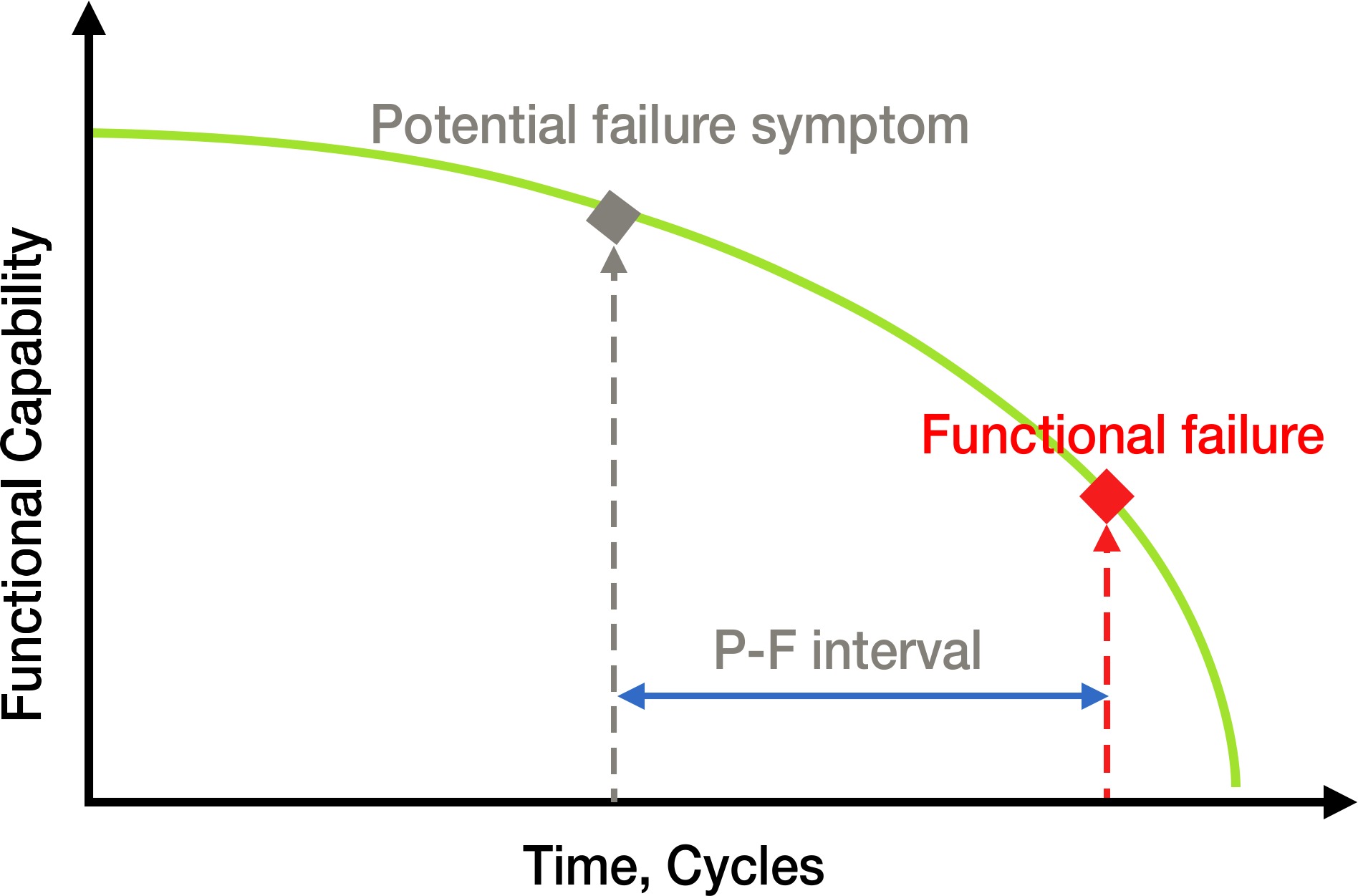
When failure mode modelling is completed, the obtained analytics can be injected within the predictive maintenance analytics framework. The capability to model accumulated damage and expected growth of each specific failure mode allows to predict accurately the time to failure. The estimation requires to define the range of damage growth by establishing which is the status to be considered as failure mode initiation and the limit of damage accumulation representing the failure condition. The range is defined then as a potential-to-functional failure interval (P-F interval) that is the time between the failure mode initiation and the accumulated damage at failure condition, as shown in Figure 3.
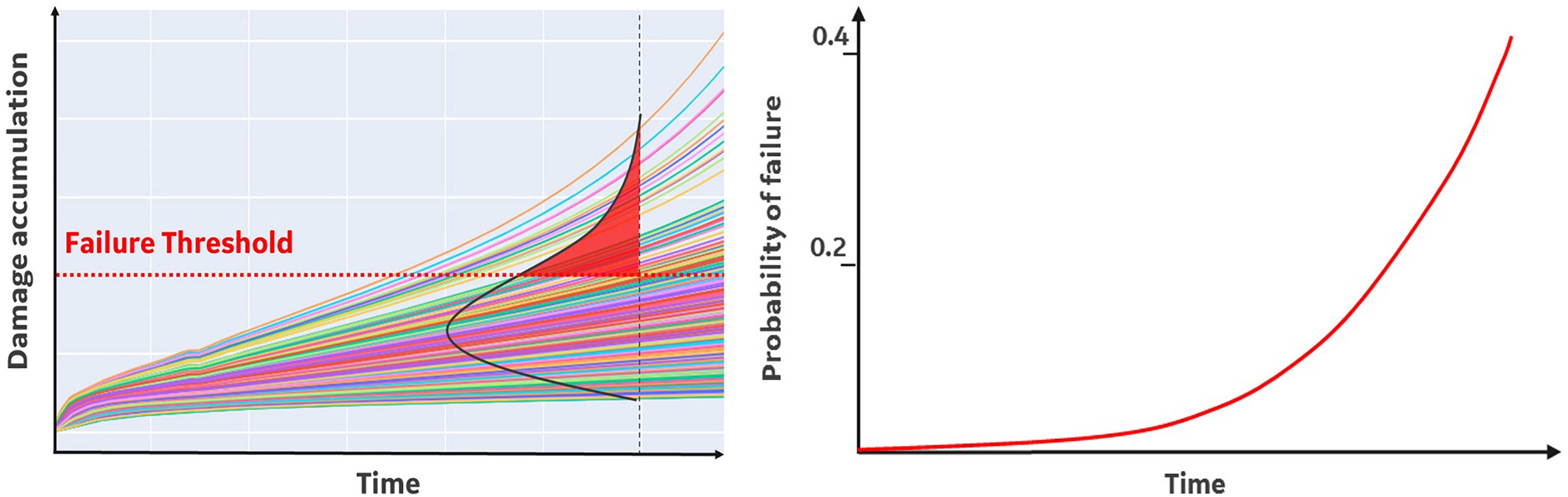
The capability to identify accurately initiation and final failure conditions depends respectively on anomaly detection accuracy and on design engineering knowledge combined with empirical experience (Escobedo et al., 2020). Having defined the P-F limits as the expected failure mode growth range, the estimation of the time to failure can be performed applying the transfer functions built during model’s development phase. The hybrid approach, leveraging on physics, ensures the forecast is executed considering the shape of damage growth that is specific of the identified failure mode: e.g. linear, exponential, logarithmic. Forecast analysis accounts for uncertainty of sensors measurements and analytics. Damage prediction at a single time sample is not a unique value but is represented by a statistical distribution that grows over time due to uncertainty propagation. The probability of failure at a certain time is the total area of the predicted values distribution above the failure limit (Figure 4).
Figure 4.
Calculation method of probability of failure versus time. Plot on the left shows the distribution of failure mode growth with uncertainty propagation over time. Plot on the right shows the probability of failure calculated as the area of damage accumulation distribution above a defined failure threshold.
With the probability of failure calculated over the entire expected life-cycle, the risk assessment is obtained by weighting the probability with impact of failure on the asset functional and operational model. The risk analysis considers also the interactions of the different failure modes within the overall engine functional diagram, combining all the reliability contributors from component level to system and asset level (Figure 5).
Figure 5.
Analysis of failure modes interaction and risk modelling from component level to unit level.
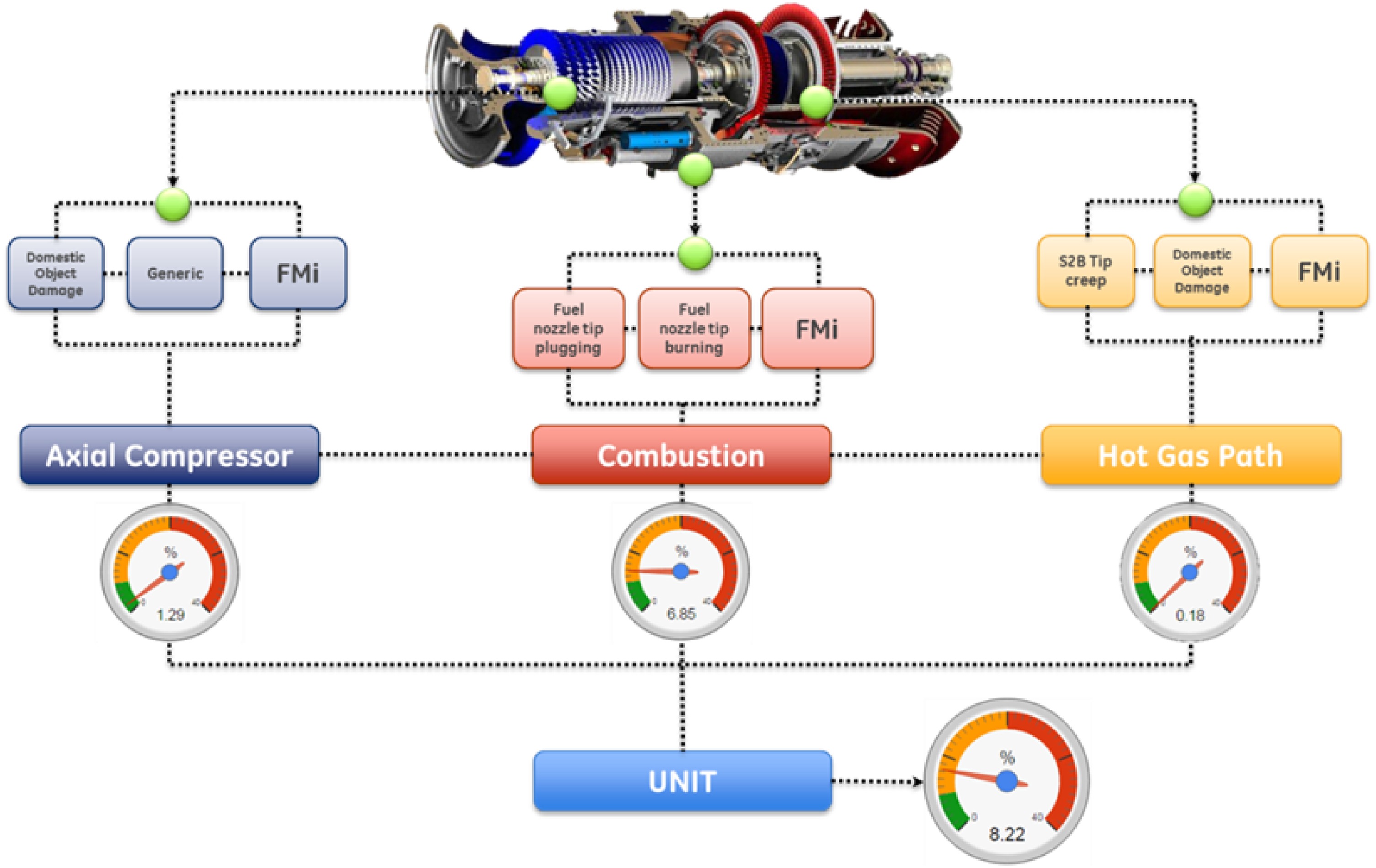
The failure mechanism of the asset depends on how the different failure modes interact with surrounding systems functionality, also considering the secondary damages caused by a single component failure. Mathematical reliability formulation considers series and parallel combination of failure mechanisms. Series combination is applied when failure modes are independent and every single phenomenon can cause the final failure of the system. In this case, the total reliability of the asset is always less than the single system reliability.
In parallel configuration, the system works as long as not all the components fail. In a parallel configuration the total system reliability is higher than the reliability of each single component.
Prescriptive layer
The outcome layer of predictive maintenance framework is intended to provide dispositions for an optimized maintenance planning, by identifying and prioritizing actions to be performed by field operators. The prescriptive layer analyses the ranking of anomalies and failures mode identified at the previous steps, with the obtained risk assessment and time to failure estimation. It is leveraging entirely on domain knowledge, fleet experience and asset functional modelling. For each failure mode, the analytics identify the most likely successful dispositions extracted from a library of historical prescriptions and collected feedback. The library is continuously updated with new cases and it reports, for each failure mode, maintenance actions performed and feedbacks that site operators and diagnostic analytics provide on the effectiveness of executed actions. Actions planning is defined leveraging on maintenance policies that define the procedure, expected effort and timeline of each maintenance task suggested by the prescriptive layer. Maintenance optimization is performed by prioritizing activities in accordance to risk ranking and grouping actions that can be performed in parallel within the same action timeframe, in order to reduce engine downtime and maximize maintenance intervals on a risk basis approach.
Results and discussion
The presented results refer to the effectiveness of predictive maintenance analytics framework, with focus on the benefits of data-driven analytics application. Within the hybrid modelling schema proposed, Baker Hughes, can leverage om the capability to use Big Data and Machine Learning to increase modelling capabilities and coverage, while physics-based approaches are well consolidated because they rely on design engineering and domain knowledge available to turbomachinery manufacturers. Thus, the results of predictive maintenance framework are presented here following by reporting use cases where data analytics contribution has maximized the accuracy of functional health assessment and failure mode modelling.
Functional health assessment
The analytics framework developed has demonstrated the capability to enable prognostics for the maintenance optimization. Here we present an example of anomaly detection and classification analytics applied for functional health assessment of gas turbines and linked auxiliary systems.
The analytics have been trained on a library of anomalies experienced on historical signals: signal freezing, step-change, spikes, noise, asymmetric noise and abnormal range. The anomalies have been replicated through signal processing in order to have the proper amount to anomalies for each class (Figure 6).
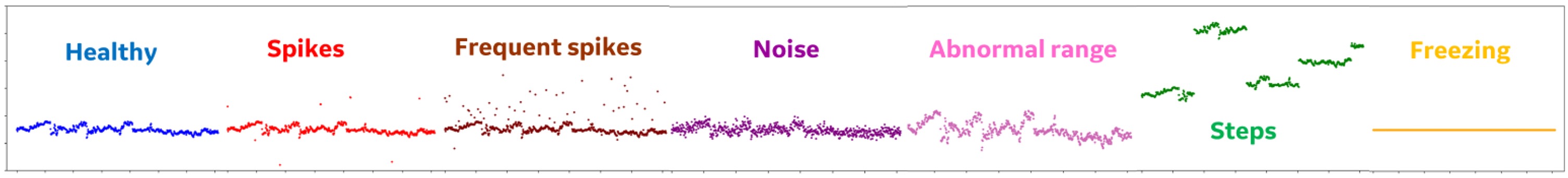
The training has been executed considering one year of data from running conditions of a group of twenty-five units. The procedure is totally automatic, requiring only to select the period of data and the set of hyperparameters to be tuned for the applied Machine Learning analytics. The training procedure automatically identifies the similarities among the gas turbine fleet, selecting the reference healthy conditions and characterizing anomaly signatures. The input dataset consists of about one hundred of signals of gas turbine and related auxiliaries. Analytics performances have been tested in the subsequent three years of data of the same engines, showing good stability and full coverage of identified critical systems and components. Performances are stable within the three years of testing window and time to failure estimated on historical events is in accordance to timeline of failure occurrence.
Examples of anomaly detection and classification catches are shown in Figure 7.
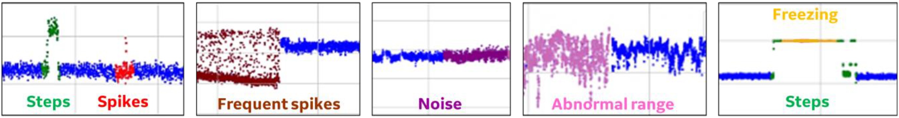
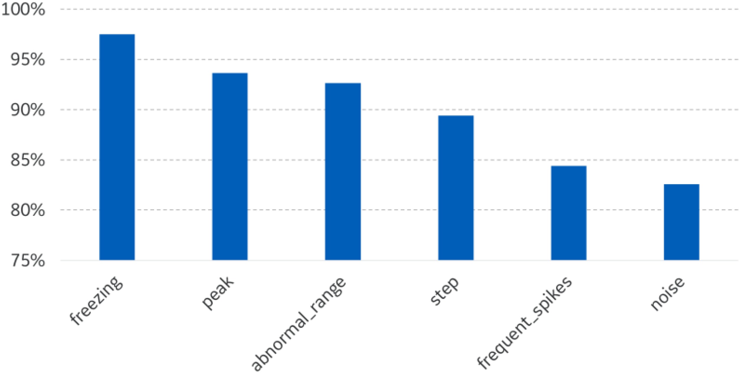
The plotted examples show the capability of the analytics to accurately detect anomalies at the very early stage. The performances obtained depend on the correct execution of model training; in particular, the timeframe selected for training must contain good references of healthy and anomalous conditions of turbine operation, allowing the algorithm to learn how to distinguish signal healthy trend from anomalous behaviour. The capability to classify detected anomalies is also related to training goodness because it depends on the examples of anomalies classes provided to the analytic, that should be as close as possible to real anomalies signature. The analysis of classifier’s performances shows that the model has an overall high confidence in identifying the anomalies, with better capabilities to classify anomalies that have a clear statistics signature with respect to anomalies having higher variance of signatures (Figure 8). For example, the classifier is extremely confident in recognizing signal freezing anomaly because a flat signal has a clear signature, while the algorithm has less confidence in recognizing noise because this anomaly can have many statistical signatures: higher standard deviation, different value distribution, digital conversion error, etc.
Furthermore, the developed anomaly detection relies on statistical features extracted from acquired signals and the resulting performances change in accordance to parameters chosen for the analysis. Accuracy of the detection depends, for example, on statistical features chosen (e.g. standard deviation, skewness, kurtosis) and on signal sampling and timeframe considered. The results have demonstrated that the statistical approach is robust if applied to slowing degradation and aging phenomena, while the choice of sampling and timeframe window impacts the detection accuracy of fast events (e.g. occurring in less than one week).
Failure mode modelling
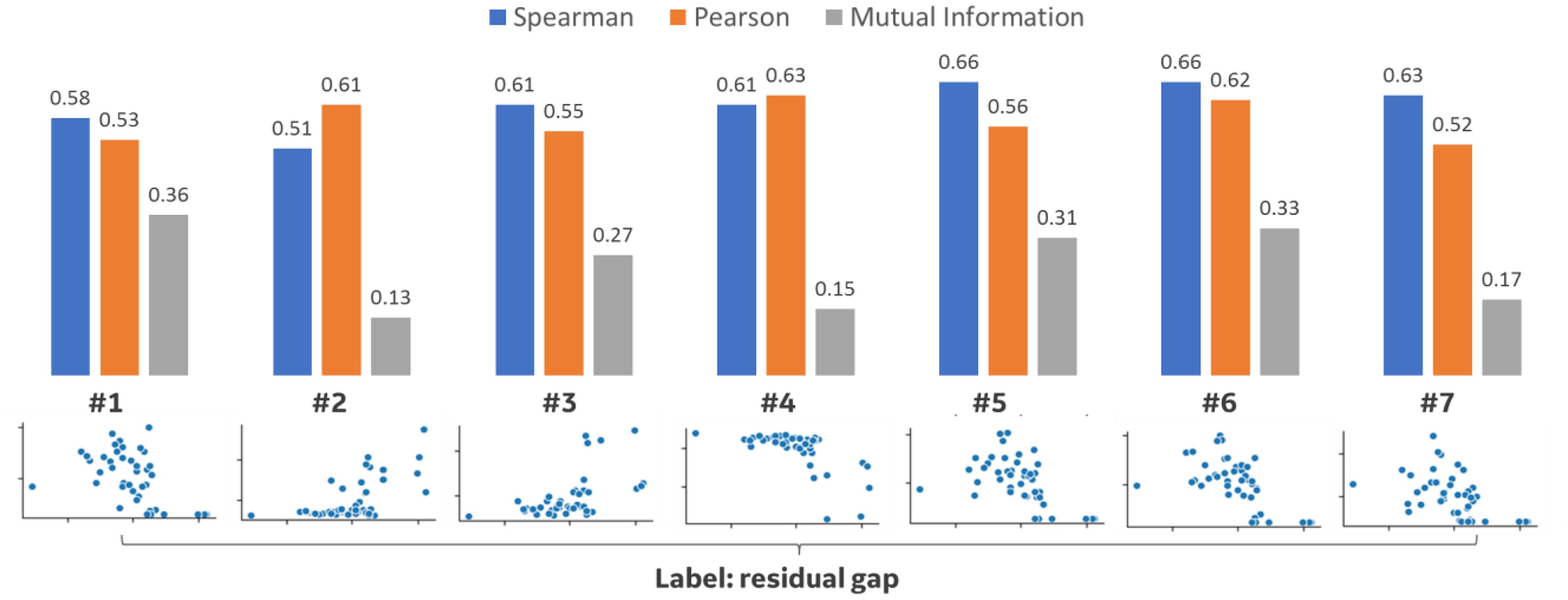
The failure mode modelling capabilities have been tested on a creep deformation phenomenon experienced on gas turbines. The failure mode can lead to final contact between rotating and fixed components. The available data are represented by acquired timeseries and defect measures taken at inspection intervals. The output labels are measures of residual gap between the components and the ranking of creep severity expressed in low, medium and high classes. The test case presented is among the worst cases for predictive maintenance applicability, because the model accuracy is affected by the impossibility to model the physics complexity and the data availability is limited. The model represents a data-driven transfer function between engine operational parameters and damage growth, collected for about fifty engines. Although the impossibility to model the physics of the failure mode phenomenon, the injection of domain knowledge can be used to increase the information content of the inputs. Thus, the first step of modelling is the execution of physics-informed features engineering where physics is applied to calculate relevant features of the failure mode phenomenon. After the data augmentation step, the input timeseries have been processed to obtain life aggregated features to be compared with the labels. The comparison has been executed studying correlations and mutual information metric, combined depending on features and label data type. Figure 9 shows an example of comparison between correlations with Mutual Information metrics, where it is highlighted how Pearson’s and Spearman’s correlations can capture respectively linear and non-linear correlations while Mutual Information identifies distribution similarities.
Figure 9.
Comparison of Pearson’s, Spearman’s correlations and mutual information metric for input features selected. The bottom graphs show the plot of selected features versus the output label value (residual gap). The upper bar-plots show the values of Pearson’s, Spearman’s correlations and mutual information metric.
Features selection step allowed to select seven relevant features starting from a dataset of hundreds of attributes. With the selected relevant features, the data-driven modelling of failure mode growth has been performed. Common methodologies for regression and classification have been compared. For all the models an initial step of hyperparameters tuning has been executed, applying k-fold cross validation that is helpful when dealing with small datasets. The algorithms that have shown the best results are Gradient Boosting for residual gap regression and Random Forest for creep severity classification (Figure 10). In particular, the estimation of residual gap performed with Gradient Boosting algorithm has an error equal to 28.5% of the failure growth range, meaning the model has more than one third of discriminant capability with respect to damage accumulation estimation. The error percentage estimation is performed by comparing the Mean Absolute Error (MAE) with the statistical range of normalized residual gap (2-sigma range considered). The classification of creep severity performed with Random Forest algorithm has shown balanced accuracy equal to 83% (Table 1).
Figure 10.
Best regression and classification models obtained for the studied creep failure mode. Plots show model prediction for train (black dots) and test samples (blue dots), compared with the expected values (green line). Plot on the left shows Gradient Boosting regression for normalized residual gap label; the obtained MAE is 0.57 sigma, representing 28.5% of the failure mode growth range (2-sigma). Plot on the right shows the Random Forest classifier for creep severity expressed in a numerical scale 1–3 (low, medium, high severity); obtained balanced accuracy is 83%.
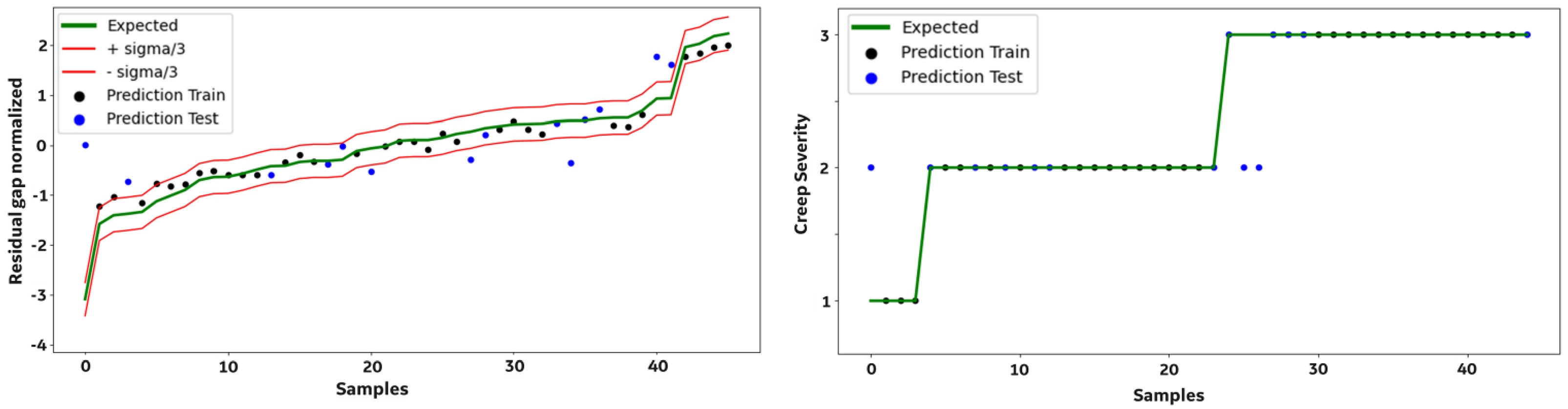
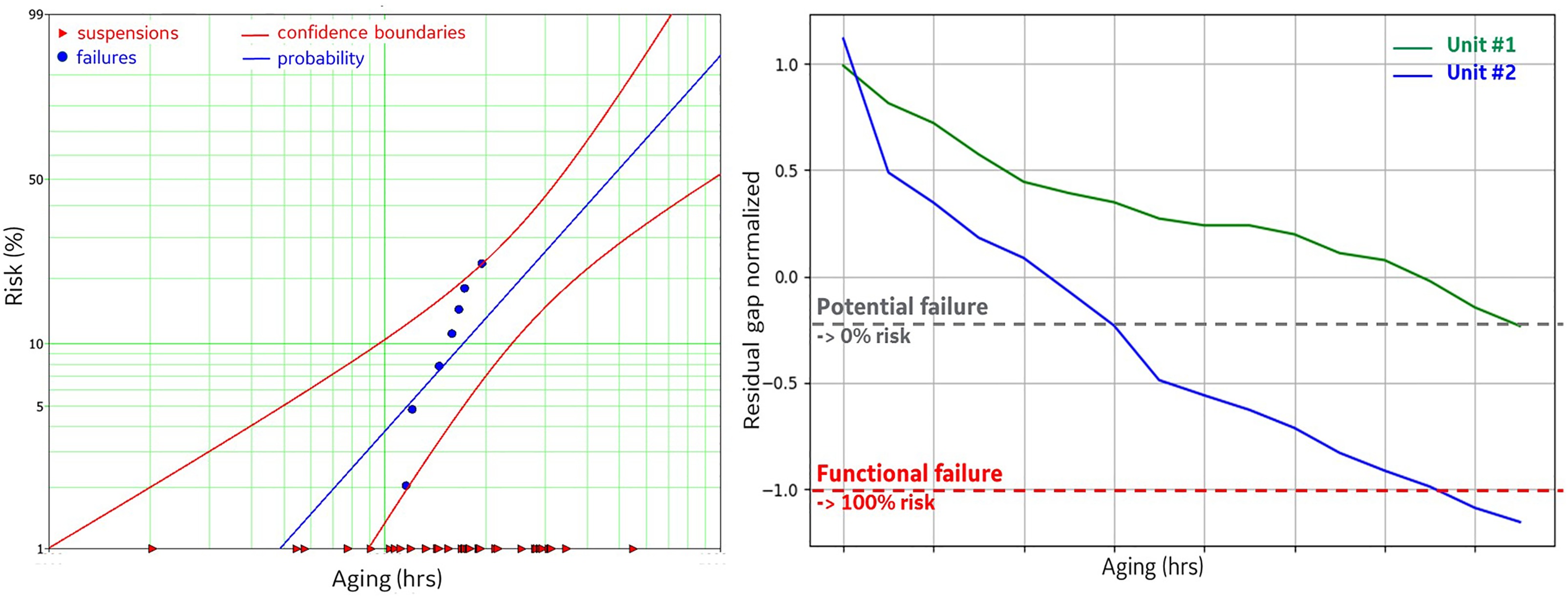
The obtained performances for both regression and classification algorithms show that obtained accuracy is acceptable but not optimal. The cause is the noise in the input dataset; the collected damage measures are probably affected by measurement error and design tolerances that would need more samples collected to be properly addressed. Overall, the models have demonstrated a discriminant capability of the damage estimation sufficient to predict the damage growth rate and to plan the maintenance accordingly. In general, ensemble methods have performed better on the selected dataset with respect to single methods, because their better capability to minimize bias and variance errors. Boosting techniques tend to overfit noisy data but a robust hyperparameters tuning can prevent this issue. In this scenario, classical approaches like reliability modelling of failure rate versus time, would have provided poor prognostic performances, estimating the probability of failure but without any capability to assess the accumulated damage and the growth rate. Indeed, classical methods of reliability modelling are able to predict the probability of failure at fleet level, with poor capability to address the engine-to-engine variability (Figure 11). The new approach is able to describe the damage severity and growth with respect to the historical behaviour and the specific operating profile of the single engine, recognizing the relevant features that impact the failure growth, with the possibility to modify the engine operation and slow-down the damage accumulation rate. The improvement is the capability to estimate the residual life for each specific engine, assessing the engine-to-engine variability and provide useful insights to optimize operation and maintenance (Figure 11).
Figure 11.
Comparison between classical and new risk modelling approaches applied to the failure mode under analysis (creep deformation). The plot on the left shows the classical approach of reliability analysis though a Weibull model, where the probability of failure is a function of engine aging and it represents the expected failure rate over time (failures represent the engines with damage size above the serviceable limits, while suspensions are the units found serviceable or healthy). The model is useful to describe the expected rate of failure among a fleet of similar units with no capability to model engine-to-engine variability. The plot on the right shows an example of the new risk modelling approach where the model is able to estimated directly the failure mode size, differentiating the estimated values in case of engines with equal running hours but operated differently (engine-to-engine variability is modelled). The risk of failure is obtained comparing the accumulated damage with the potential and functional failure thresholds.
Results demonstrate the applicability of the developed analytics framework to turbomachinery predictive maintenance applications, thanks to accuracy improvement guaranteed by hybrid modelling applied to anomaly detection and prediction of time to failure.
Conclusions
The evolution from preventive to predictive maintenance requires to assess health status, detect and monitor failure modes and predict time to failure of turbomachinery assets. The key differentiators of the predictive approach are anomaly early detection capabilities and accuracy of prognostic analytics. Because the complexity of turbomachinery reliability modelling, the accuracy target needs to be achieved at each modelling step, starting from the signal anomalies detection, continuing with systems functional modelling and closing with risk assessment of asset failure. Otherwise, inaccuracy of each single model propagates through the multilevel asset model and it results in reduced confidence of risk assessment and time to failure estimation.
Baker Hughes proposes a predictive maintenance method tailored in a multi-level analytics framework that starts from the anomaly detection, which triggers the failure mode identification and the consequent risk assessment for an optimized maintenance scenario. The availability of big data from online monitoring and advanced inspections fills the accuracy gap of the classical preventive maintenance approach where risk assessment was performed on the basis of domain knowledge and fleet experience with limited usage of online monitoring data, leading to track fleet statistics with limited capability to model the specific asset behaviour and engine to engine variability. The merge of data analytics with physics-based modelling is optimizing prognostic capabilities, achieving the requested accuracy target and it allows to describe the complexity of asset functional and health models. For example, functional anomalies usually produce characteristic signatures on acquired sensors measurements and can be detected at the very early stage though data-driven analytics. Many other failure modes relate to material degradation or component distress that do not result in asset or system malfunction, remaining undetected till the final component failure. Transfer functions between engine operational data and damage accumulation have to be developed to model relationship between online monitoring data and offline measurements taken at inspections intervals, when failure modes are identified and the related damage quantified.
The paper presented the application of hybrid modelling in the worst-case scenario where physics knowledge is limited and sensor measurements are far from the object area. Data-driven approach is used to model the failure mode and physics is injected in the input dataset to calculate relevant features used to predict the damage growth. The prediction accuracy is improved with respect to standard reliability modelling of failure occurrence rate, with increased discriminant capability of damage accumulation and growth rate. With an accurate prediction of time to failure, turbomachinery domain knowledge and maintenance expertise are applied to optimize actions plan based on risk assessment.