
Introduction
Virtual prototyping based aerodynamic design procedures in aeronautics, propulsion and power generation systems are still overwhelmingly of deterministic character. They neglect the influence of uncertainties that originate from the manufacturing process. The computer-based design analysis by Computational Fluid Dynamics (CFD) is done on a CAD based geometrical model, ignoring the inevitable manufacturing variability that is inherent to every manufacturing process. The admissible manufacturing tolerances resulting from geometrical deformation by casting, heat treatment or the machining processes are not accounted for in the simulations, which leads to design choices that have an unknown behaviour with respect to these uncertainties.
Methodologies to quantify the impact of manufacturing uncertainties in 3D CFD based design strategies were for a long time computationally unaffordable on real world industrial applications. Over the past decade uncertainty propagation methods have been developed that reach levels of industrial applicability such as non-intrusive polynomial chaos and sparse polynomial chaos methods based on both quadrature and regression (Xiu and Karniadakis, 2003; Najm, 2009; Blatman and Sudret, 2011; Abraham et al., 2017), collocation methods (Mathelin and Hussaini, 2003; Loeven et al., 2007), or Monte-Carlo and Multi-Level Monte-Carlo methods for which an overview can be found in (Schmidt et al., 2019). Intrusive polynomial chaos (Smirnov and Lacor, 2008; Dinescu et al., 2010) and perturbation methods also received attention (Dervieux, 2019).
Some of these methods are integrated into toolsets that allow for quantification of operational und geometrical uncertainties on industrial scale simulations such as described in (Wunsch et al., 2015), where a significant reduction in computational cost is achieved by a sparse grid technique (Smolyak, 1963). To address optimization under uncertainties, this uncertainty quantification (UQ) method is combined with a robust optimization approach, which relies on a mixed design space covering the geometrical variability and uncertainties (Poulos et al., 2017; Nigro et al., 2019a).
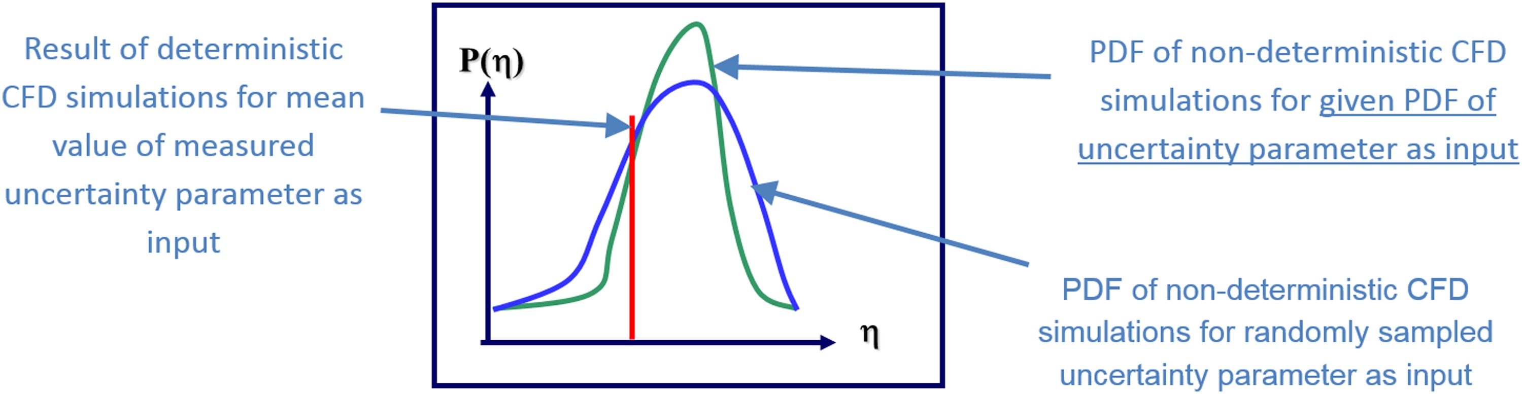
By introducing the probabilistic nature of uncertainties in the simulation based design process, the governing equations transform into stochastic partial differential equations that are solved with methods such as the ones listed above. A key consequence of this approach is that predicted quantities such as loads, drag, efficiency, etc. are not single values anymore but probability density functions (PDF). Figure 1 illustrates this fundamental change. The red line indicates the value that is obtained by standard deterministic simulations that ignores the influence of uncertainty. Here the mean value of the measured input uncertainty is used as input to the simulation. The green curve shows the result of a non-deterministic simulation where the measured distribution of the input uncertainty is provided as input to the simulation. The first observation is that its mean value is different from the output of the deterministic simulation. This is a consequence of the non-linear response of the simulated system over the range of variability of the input uncertainty. In CFD the simulated system of equations are the Navier-Stokes equations and only for very small input uncertainty variations a close to linear response can be observed. A second main observation is that the prediction of the system is different, if the input is sampled randomly as shown by the blue line. The characterization of the input uncertainty is crucial to the non-deterministic simulation approach. This characterization of input uncertainties and their application to uncertainty quantification and robust design optimization (RDO) is at the core of this contribution.
Characterization of input uncertainties in industrial design is a challenging task and these challenges can be very different in function of the industry or application. An aircraft manufacturer might turn out a low 2-digit number of aircrafts per year for some aircraft types. If uncertainty on components like the wings should be considered, the time to sample a sufficiently large number of actually manufactured wings to build a statistically converged data set might take a few years. Measuring a few hundred compressor blades of an aircraft engine to sample the manufacturing variability is considered a reasonable data set size. But what are the options for custom built machines, where the sample size will never be sufficiently high for the task of characterization of input uncertainties? A possible path to the characterization of manufacturing input uncertainties is described in (Büche et al., 2019) and adopted here. It is based on deriving input uncertainties from technical norms that determine the general tolerances in manufacturing such as ISO 2768-1 (1989).
On the basis of this norm, manufacturing tolerances are derived for a high-pressure turbine blade and then virtually sampled. A Principal Component Analysis (PCA) is then applied on the sampled geometries to determine the principal modes of deformation of the geometry independent of the geometry parametric description. In the case of many uncertainties it can be used to reduce the complexity of the problem, by representing the same geometrical variability with less variables. It is also used to gain physical insight into the influence of the deformation modes. Then the technical norm based method for characterizing manufacturing input uncertainties is applied to a marine propeller for which an optimisation under uncertainties is performed.
Methodology
In the following sections, the derivation of manufacturing variability from technical norms is discussed and the virtual sampling method is described as well as the application of principle component analysis. The last section describes shortly the applied uncertainty propagation method to the extent to which it is directly relevant for the understanding of the work described here.
Derivation of manufacturing uncertainty from technical norms
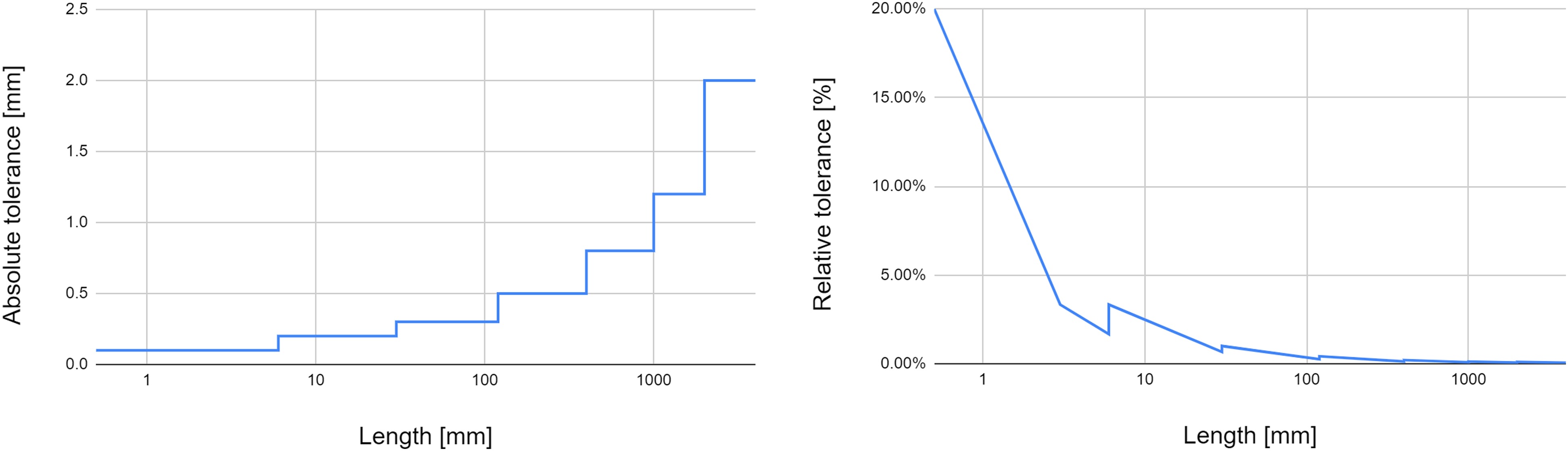
Following (Büche et al., 2019) the norm relevant to general manufacturing tolerances (ISO 2768-1, 1989) is used to illustrate the principle. Table 1 shows the permissible tolerances in (mm) for four different tolerance classes from “fine” to “very coarse”. Figure 2 is an illustration of the class “medium”. The first observation that can be made is that the absolute value of the tolerance increases with the linear dimension. While for the class “medium” the permissible tolerance is ±0.1 mm for a nominal length ranging from over 3 to 6 mm, the permissible tolerance is ±1.2 mm for a nominal length ranging from over 1,000 to 2,000 mm. This is also illustrated in Figure 2 (left). Figure 2 (right) shows the relative tolerance in (%) over the nominal length. It is seen that while the absolute value is small for a short nominal length, the relative tolerance can reach up to 20%. Components with small linear dimensions might thus be affected by larger uncertainty. One could argue that because the dimension is small it is of less influence on the machine performance. This is however a wrong assumption as will be shown when analyzing the influence of the deformation modes on the high pressure turbine further down.
Table 1.
Tolerance classes for linear dimensions from (ISO 2768-1, 1989).
Computer aided designs (CAD) of components such as turbine blades or marine propellers is usually done on the basis of a given parametric description describing lengths, radii and angles of the geometry. This parametric description is exploited in the following to define the manufacturing tolerances and sample the geometries virtually on the computer.
Virtual sampling of manufacturing variability and Principal Component Analysis
The virtual sampling method for manufacturing variability and subsequent PCA can be described in the following steps:
Derivation of manufacturing tolerances for the individual geometrical parameters
Definition of uncertainties on all parameters (type of uncertainty)
Perform a design of experiment (here a Latin Hyper-Cube Sampling) that generates O(1,000) geometries
Build a covariance matrix based on these geometries
Solve the eigenvalue problem. The resulting eigenmodes become the uncertain variables and the eigenvalues the variance of these uncertainties.
The number of retained modes can be truncated and only a reduced number of uncertainties is retained.
After the manufacturing tolerances are identified for all parameters in function of the appropriate tolerance class (step 1), types of distribution need to be attributed to these uncertainties. This step requires some insight into the manufacturing process and the type of distribution can be informed by past experience or simply be assumed. In any case the sampling method (step 3) needs to be compatible with arbitrary PDF shapes. To unify the sampling of a Design of Experiment (DoE), the sampling is performed over the Cumulative distribution function (CDF) instead of the PDF. This allows for a uniform sampling over the parameter range, which is for every CDF in the range [0, 1]. Figure 3 (top) shows that sampling uniformly from 0 to 1 for a uniform distribution results in uniformly distributed sampling points. Figure 3 (bottom) shows that sampling uniformly from 0 to 1 for a symmetric beta distribution results in sampling points that respect the probabilities of a beta distribution.

A Latin Hyper-Cube sampling is then performed on the CDF distributions according to the characterized manufacturing uncertainties. This generates O(1,000) geometries in an automated loop over the design or CAD tool used to build the geometries. They are topologically similar, which eases the computation of the geometry covariance matrix (step 4). Then a PCA is applied to the covariance matrix computed from the virtual geometry sampling (step 5) and the resulting eigenmodes become the uncertain variables, while the eigenvalues represent the variance of these uncertainties. Finally, the number of retained modes can be truncated to retain a variable amount of geometrical variance. This is done for several values of retained variance resulting in separate UQ problems with an increasing number of uncertainties. These are then compared to the full UQ problem. The methods used to propagate these uncertainties are described in the following section.
Uncertainty quantification, scaled sensitivity derivatives and robust design optimization
Uncertainty quantification
The uncertainty propagation method used is the non-intrusive probabilistic collocation method by (Loeven et al., 2007). The chain of methods is available in FINE™/Design3D (NUMECA, 2019) and used here. The methodology is described in detail in (Wunsch et al., 2015), but the main elements are reprinted here. If a generic stochastic partial differential equation is considered such as:
with L being a differential operator containing space and time derivatives, S being the source terms and
where,
with:
Once all Np computations are performed, the first four moments of any output quantity
For several simultaneous uncertainties multi-dimensional quadrature can be done by tensor products. This leads, however, to an exponential increase in the number of points with the number of dimensions, the so-called “curse of dimensionality”. Sparse grid quadrature can overcome this curse of dimensionality to a certain extent and make non-intrusive collocation methods accessible for higher stochastic dimensions. The implementation is based on Smolyak’s quadrature (Smolyak, 1963). This reduces the cost for an accurate prediction of mean value and variance for 10 simultaneous symmetric beta distributed uncertainties from 59,049 to 21 CFD simulations.
Scaled sensitivity derivatives
The relative influence of a given uncertain input on the solution of the system is determined by calculating scaled sensitivity derivatives (Turgeon et al., 2003). This is applied here to the probabilistic collocation method. The scaled sensitivity derivative is defined as the partial derivative of the solution
Robust design optimization
For robust design optimization the UQ method is coupled with a surrogate assisted online optimization procedure (NUMECA, 2019). The optimization objectives and constraints are not single values in robust optimization, but the mean value and standard deviation of the quantities of interest. The most straightforward approach would be to run full 3D CFD based UQ simulations for every point in the Design of Experiment (DoE) and calculate a surrogate for the statistical moments. This is, however, very costly since a database usually contains hundreds of points. At the example of 10 simultaneous uncertainties, a DoE of 200 samples would require 4,200 CFD simulations, which is hardly feasible. A mixed DoE comprising both the design variables and the uncertainties is used here (Poulos et al., 2017; Nigro et al., 2019a), which reduces the computational cost significantly.
Results and discussion
The above described methodology is first applied to a high-pressure turbine. Manufacturing uncertainties are characterized and sampled based on the relevant technical tolerancing norm. The PCA is applied and the influence of the sample size used to build the geometrical covariance is discussed. Then the influence of the individual modes on the prediction accuracy of CFD quantities is analyzed and it is shown that geometrical reconstruction accuracy and CFD predictions are not linearly related, which has important implications on the total geometrical variance that needs to be retained.
A second application of the characterization of manufacturing uncertainties to a marine propeller is discussed and it is shown that these uncertainties can be used for robust design optimization of the marine propeller.
High pressure turbine: Virtual sampling of manufacturing variability
The geometry investigated here is a high-pressure turbine blade that was designed with the 3D design software AxCent (Concepts NREC, 2019), which is dedicated to turbomachinery design and coupled for CFD analysis to the above described simulation chain. A pair of 4 uncertainties is chosen as uncertain variables, four uncertainties in a blade section close to the hub and four uncertainties in a blade section close to the tip of the turbine blade.
Figure 4 shows the shape of the two blade sections, where the blue profile is located close to the hub and the red profile close to the tip of the blade. Eight uncertainties are derived from ISO 2768 in 4 tolerance classes for the following parameters of the AxCent geometric model:
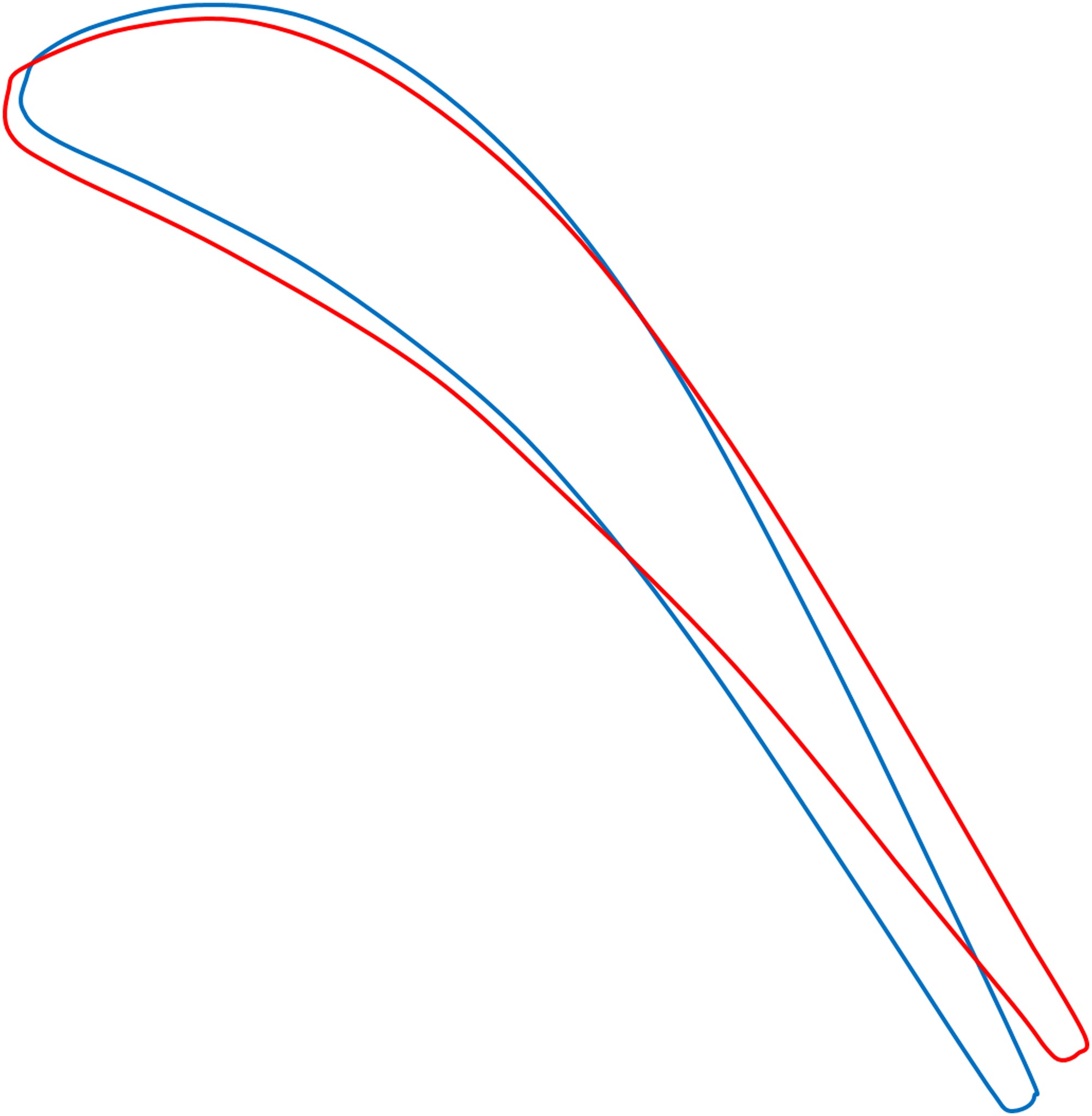
The choice of the uncertainties is based on the authors experience with UQ simulations of turbomachinery cases and literature references, given that no manufacturing uncertainties are available that result from a specific manufacturing process. The choice of the four parameters is based on the work of Nigro et al. (2019b), where realistic manufacturing variabilities derived by Lange et al. (2010) were quantified. Among the most influential uncertainties with respect to efficiency that were identified by Nigro et al. (2019b) are the leading edge radius, leading and trailing edge angles. The chord length was quantified to have a smaller impact on the efficiency. For the uncertainties that lie within the tolerance bounds defined based on the technical norm, a preliminary study didn’t show notable differences between different types of symmetric distributions inside these bounds. Table 2 shows in the first column the name of the parameter per section and in the second column its value. It is seen that the trailing edge blade angle is approximately −60.5° for the section close to the hub and −55.9° for the section close to the tip, which is also reflected in Figure 4.
Table 2.
Maximum admissible tolerances for the turbine blade parameters.
Table 2 lists the permissible tolerances for the four classes from ISO 2768. At the example of the chord length with a nominal value of 8.73 mm the admissible tolerance is ±0.1 mm for the class “fine” and ±1.0 mm for the class “very coarse”. For angular dimensions the permissible tolerances increase with decreasing nominal angles as shown in Table 2 for the trailing and leading edge angles in both sections. The trailing edge angles vary between approximately −55° and −60°, where the permissible tolerances are ±0°20′ for the class “fine” and ±1°00′ for the class “very coarse”. For the leading edge angles, however, with nominal values of approximately 2° to 3° the permissible tolerances are ±1°00′ for the class “fine” and ±3°00′ for the class “very coarse”. This corresponds to an admissible tolerance of more than 100% of the nominal value.
Simulation setup
The high-pressure turbine is meshed with 2.33 million structured full hexahedral cells generated with AutoGrid5. The CFD simulations are performed with a Spalart-Almaras turbulence model and the simulation converges in 15 min on 48 processors using the CPU-Booster in FINE™/Turbo. The convergence level is pushed further than usual to assure that even the smallest geometrical changes are taken into account. This was done out of precaution and based on the effective convergence observed after having run the simulations, the computational effort can be reduced by a factor 2. Figure 5 shows the colour contour of the relative Mach number in a cutting plane placed at 90% of the blade span position.
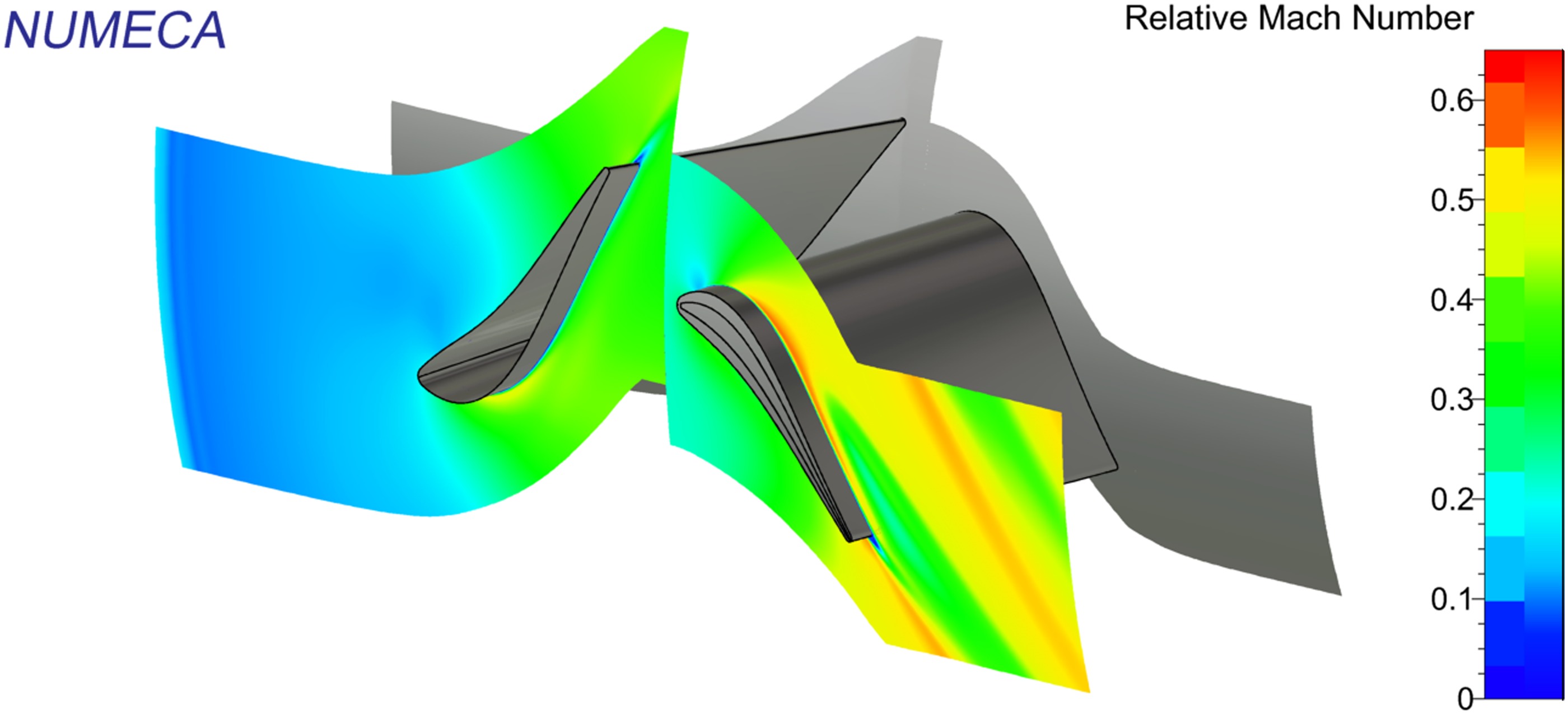
Figure 6 illustrates the influence of the uncertainties on the geometry and the flow solution. The view perspective is strictly identical for both Figures 6 (left) and (right) the small differences are due to the modification of the trailing edge blade angle. This is the only parameter that is modified here.
Figure 6.
Geometry resulting from minimum value for the trailing edge blade angle (left) and maximum value (right) at 90% of the span position.
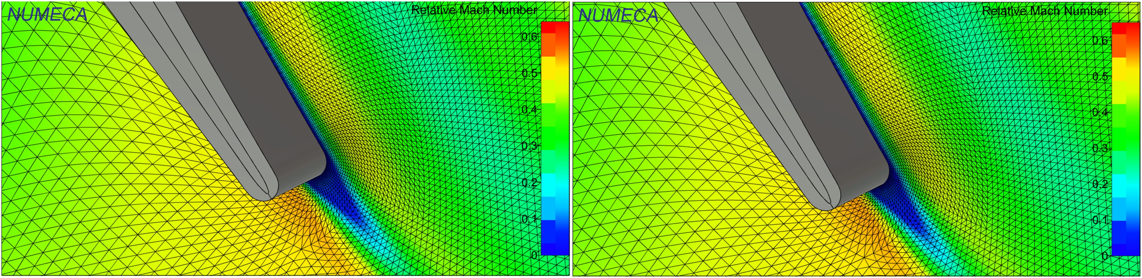
On a side note, it should be mentioned that the parametric modeller does not restrict the influence of a parameter on the geometry to a local domain of influence. As an example, modifying the chord length in the section close to the hub has also a non-negligible influence on the tip region of the blade.
High pressure turbine: Application of PCA
With the admissible tolerances identified for all the parameters describing the turbine geometry, the virtual sampling of the geometries is done by imposing truncated Gaussian distributions for all parameters that are bounded by the upper and lower admissible tolerance. As shown above any PDF shape is possible as the sampling is done over the CDF. The choice of the truncated Gaussian distribution is an assumption that does not limit the interpretability of the method.
For the PCA based method to be judged successful the reduced set of uncertain variables needs to respect the following conditions:
Predict the correct mean values of quantities of interest (efficiencies, drag, etc …)
Predict with increasing accuracy the standard deviation of quantities of interest, if more and more modes are retained
Predict the same standard deviation as the original model if all relevant modes are retained
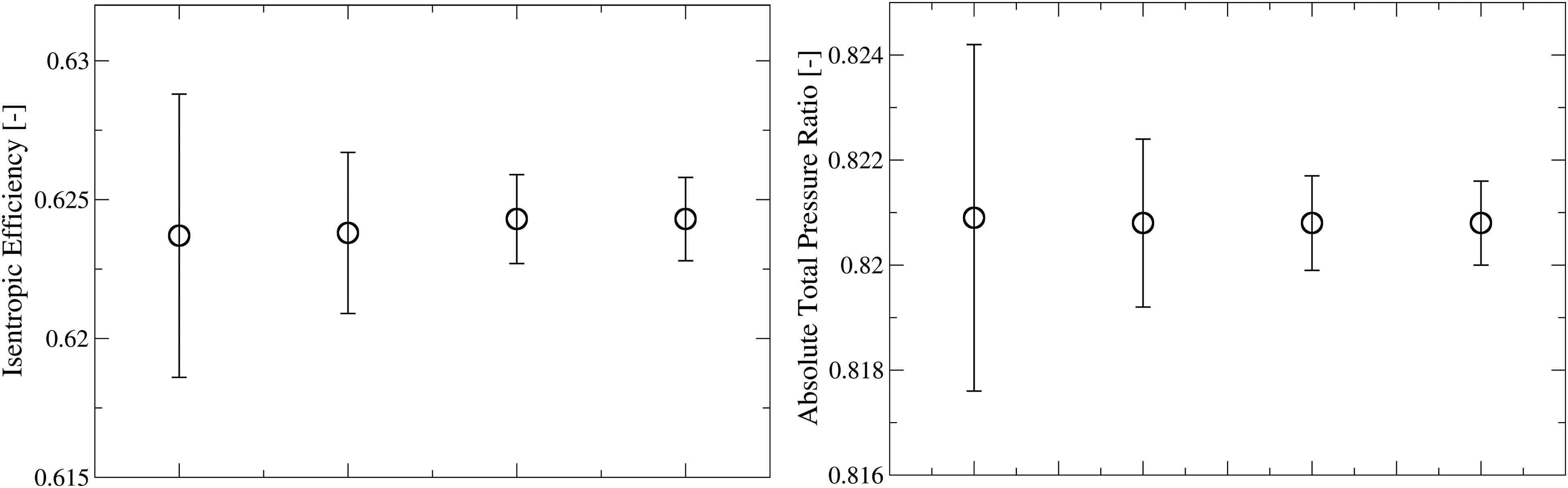
In view of these requirements, first a reference UQ solution is built and the results in terms of mean value and standard deviation of isentropic efficiency and absolute total pressure ratio are shown in Figure 7. For these results all 8 parametric uncertainties are propagated through the turbine flow. The first observation is that there is only a slight modification of the mean values for the efficiency and nearly constant values for absolute total pressure ratio with the various tolerance classes. The standard deviation, as it is expected, reduces with more stringent tolerance classes, but there is a surprising effect when passing from class “medium” to the class “fine”. The standard deviation reduces only very little. This is valuable information to the design engineer to know that decreasing the admissible manufacturing tolerances does not yield any or only very little advantage in terms of performance stability. As more stringent tolerances are connected to a significantly higher manufacturing cost. If the performances of a machine manufactured with tolerances of class “medium” are the same as for one manufactured with class “fine”, then the manufacturing cost can be reduced significantly.
Figure 7.
Evolution of the mean value and standard deviation ±1σ in function of the tolerance class for isentropic efficiency (left) and absolute total pressure ratio (right) from very coarse to fine.
These UQ results on the full system will serve as a reference for the PCA based UQ study in the following.
When applying the PCA based approach, one of the first questions to answer is the sample size of geometries required. While experimental measurements on manufactured blades are limited to a few hundred blades, the virtual sampling allows to increase arbitrarily the number of geometries. In this case up to 4,000 geometries are sampled within a few minutes. This allows for a parametric study of the influence of the sample size on the mode decomposition and the eigenvalues, which are used as variances of the imposed mode-based uncertainties. Figure 8 shows the eigenvalues obtained for 50, 500, 2,000, and 4,000 samples. By pure visual analysis it is immediately apparent that the eigenvalues are only converged for 2,000 samples. The value of 2,000 is case dependent, but it is expected to be in this range for manufacturing uncertainties characterized on the basis of general tolerancing norms.
Figure 8.
Eigenvalues obtained with sample sizes of 50 (top left), 500 (top right), 2,000 (bottom left) and 4,000 (bottom right) geometries.
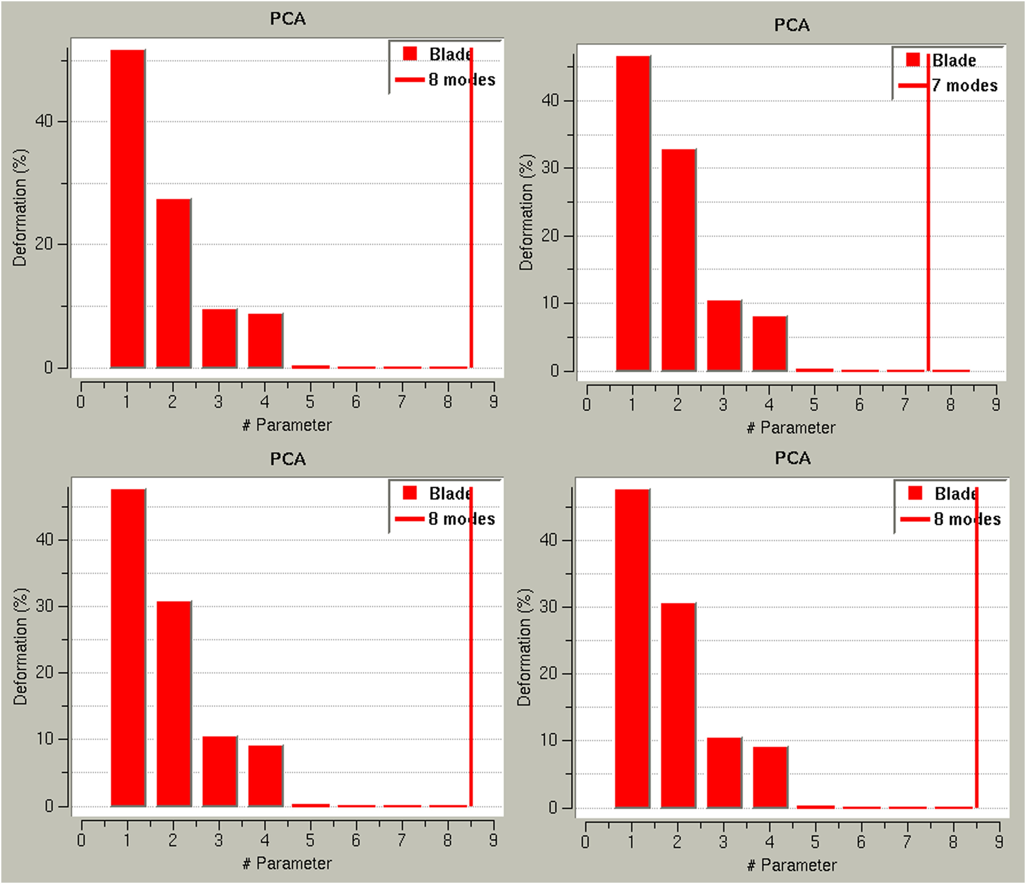
The variance that is retained per mode is shown in Table 3. To include 90% of the variance, 3 modes need to be retained, while 99.9% of the variance requires to retain 7 modes.
High pressure turbine: Discussion of mode analysis and mode sensitivity
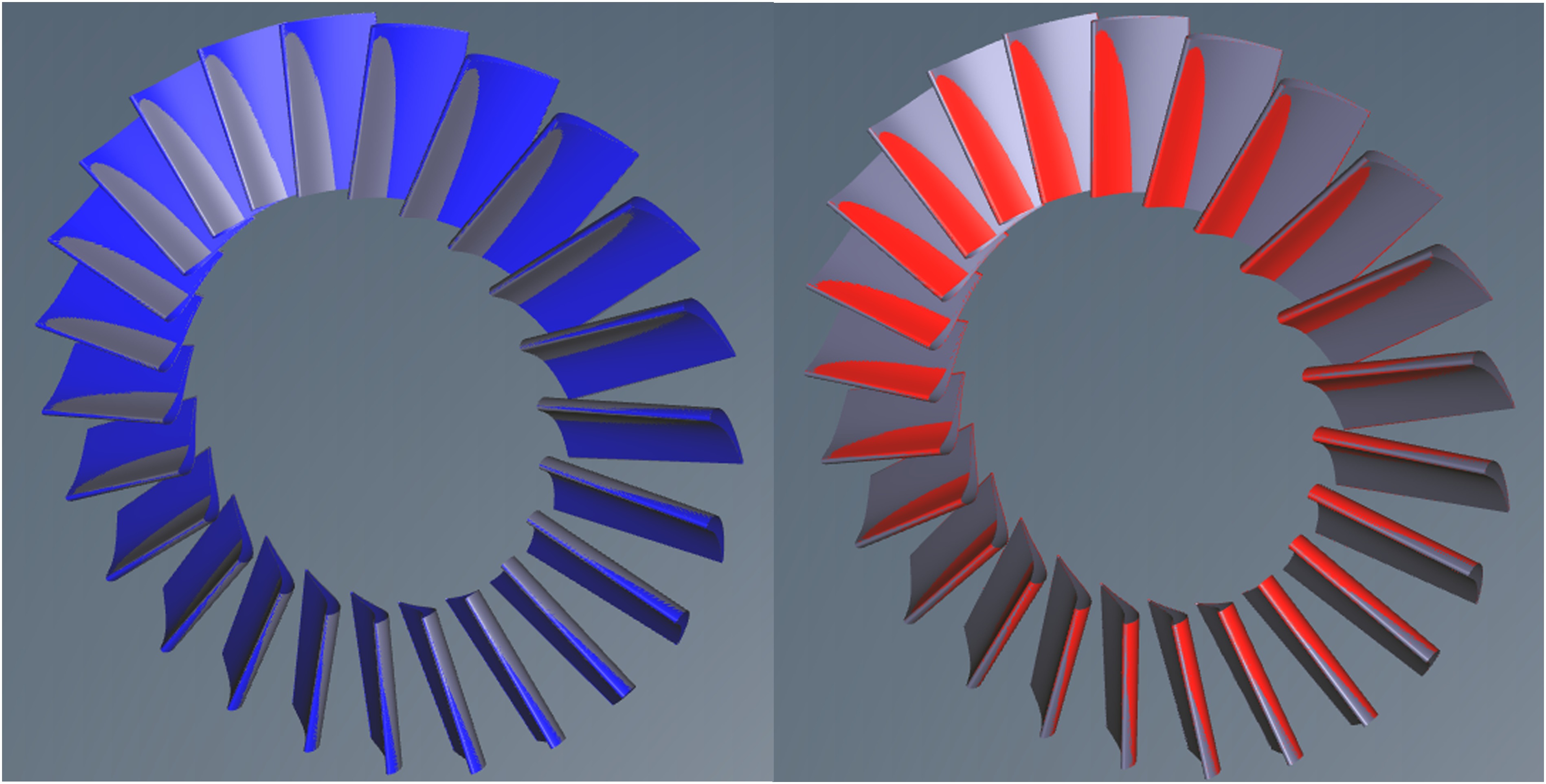
In order to get an idea of what these eigenmodes correspond to in terms of geometrical deformation Figures 9–11 show the geometrical deformation of the geometry in the direction of the respective modes and against the direction of the respective modes. Figure 9 shows that for the first eigenmode the deformation is in the order of the span height of the blade and represents thus a large geometrical variability. On both figures the non-deformed geometry is shown in grey. It is then overlaid with the geometry that results from deforming the base geometry against the direction of the first eigenmode (in blue on the left of Figure 9) and with the direction of the first eigenmode (in red on the right of Figure 9). Visually speaking, the non-deformed geometry is once “in front” and once “behind” the respective deformed geometry. It illustrates that the first eigenmode acts globally over the entire height of the blade. The same principle is applied to Figures 10 and 11. Figure 10 shows the deformation of the 2nd largest eigenmode, which appears to be in the order of the chord of the blade. Finally, Figure 11 shows the deformation due to the 3rd eigenmode. The main observation to make is that this deformation is geometrically very small and is visually difficult to identify on the figure. The main areas of deformation are located around the leading and trailing edge of the blade and cause geometrically speaking small deformations.
Figure 9.
Geometrical variability of the first eigenmode. In blue (left) deformation against the 1st eigenmode; in red (right) deformation with the 1st eigenmode.
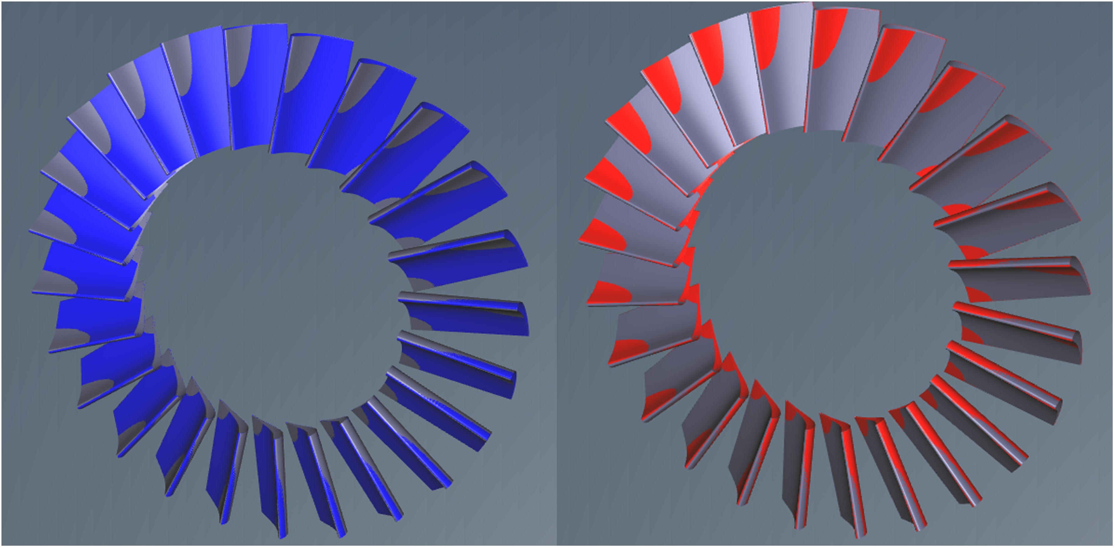
Figure 11.
Geometrical variability of the third eigenmode. In blue (left) deformation against the 3rd eigenmode; in red (right) deformation with the 3rd eigenmode.
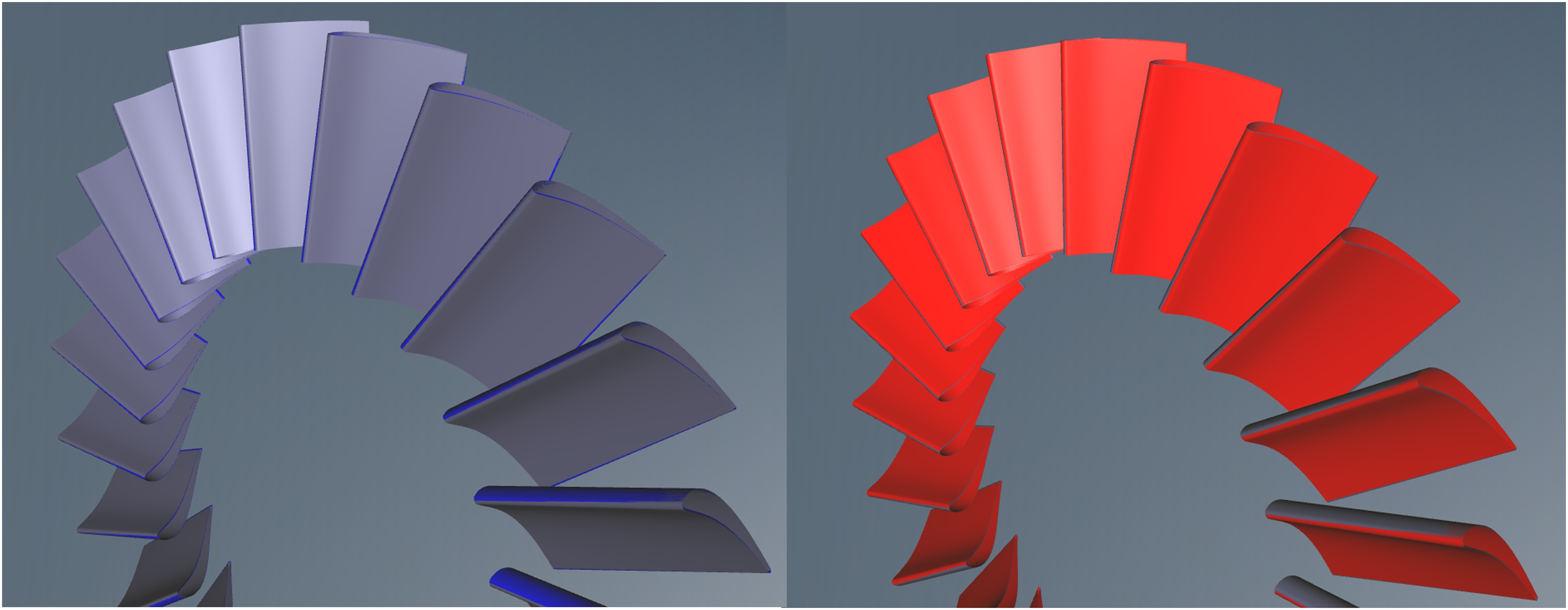
Figure 10.
Geometrical variability of the second eigenmode. In blue (left) deformation against the 2nd eigenmode; in red (right) deformation with the 2nd eigenmode.
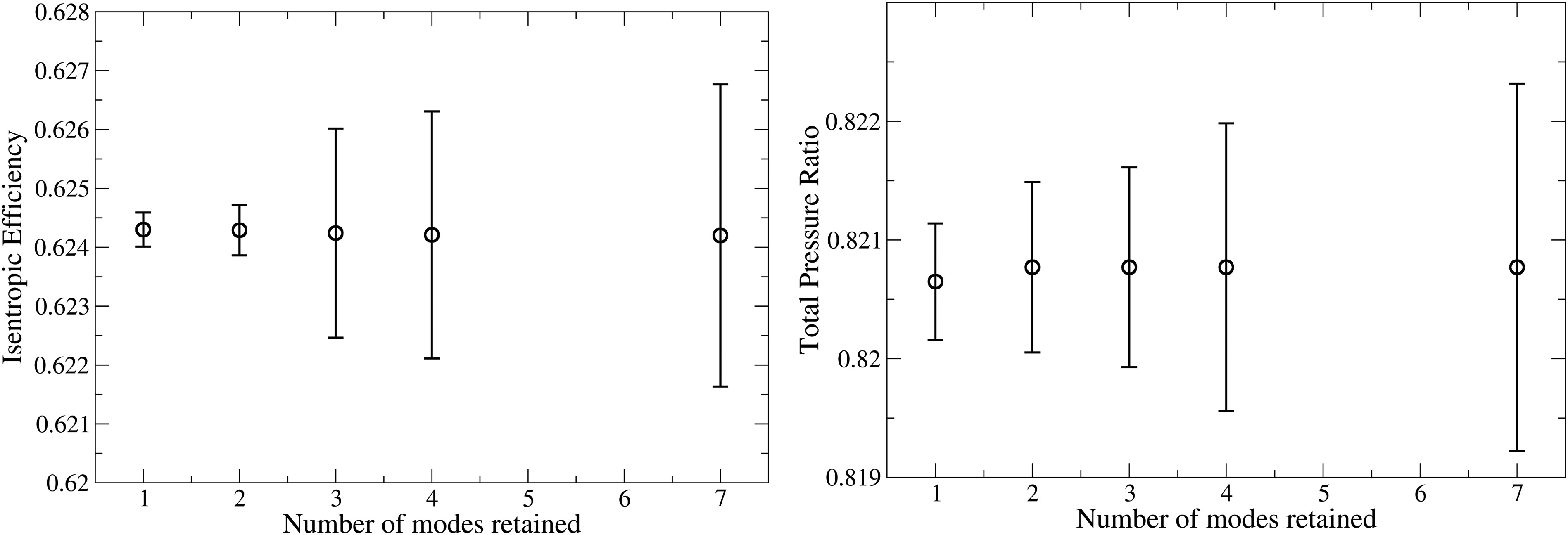
With the geometrical deformation caused by the first three eigenmodes in mind the UQ predictions with 1, 2, 3 or 7 modes retained are analyzed and shown in Figure 12. The variance that the reduced system needs to predict is the variance of the full system from Figure 7 for the respective tolerance class. Analyzing Figure 12, it is seen that the prediction of the mean is nearly constant for both quantities and across the number of modes that are retained. It can also be observed that the included variance increases with the number of modes and that the included variance converges with an increasing number of modes for all quantities. It is very interesting to have a closer look to what happens in terms of CFD prediction variance when the 3rd eigenmode is included in the UQ study. Not only that modes 1 and 2, which show by far the largest geometrical variability seem to add only little to the variance on the CFD predictions, it is by including mode 3 that significant variability is added to the variance of the isentropic efficiency. A relatively small geometrical variation has a significant influence on the prediction of the solution. This shows that the geometrical reconstruction accuracy of the deformation modes and reconstruction accuracy of the CFD predictions are not linearly related, which is something that should be kept in mind when truncations are performed on the basis of geometrical variability only.
Figure 12.
Evolution of mean value and standard deviation prediction for isentropic efficiency and absolute total pressure ratio in function of the number of modes retained.
The high sensitivity of the isentropic efficiency to the eigenmode that controls the leading edge radius can be made visible by analysis of scaled sensitivities. Figure 13 shows that the isentropic efficiency is most sensitive to the 3rd eigenmode. This is in alignment of earlier findings by Wunsch et al. (2019) that the modes retaining the largest variability of the geometry are not necessarily the modes with the most influence on output quantities.

Marine Propeller: Derivation of manufacturing variability, dimension reduction and Robust Design Optimization (RDO)
The developed methodology is applied to the characterization of manufacturing uncertainties of a marine propeller in (Vidal et al., 2019). The main results of this industrial application are summarized to illustrate its value in engineering design. The goal of the study is to optimize the propeller shape to make its performances more robust with respect to the manufacturing uncertainties.
Manufacturing tolerances for marine propellers are defined by ISO norms such as the ISO-484-2 (ISO-484-2, 2015) for any marine propeller between 0.80 and 2.50 m in diameter. The tolerances are taken from the most stringent class for the ship propeller and the relevant values are summarized in Table 4.
Table 4.
Admissible tolerances for the marine propeller.
This results in the following manufacturing uncertainties
The chord in 4 different sections (symmetric beta PDF)
The thickness distribution in 4 different sections (non-symmetric beta PDF)
The rake, which represents the linear position of the tip compared to the root of the blade (symmetric beta PDF)
The tip gap between the blade and the duct (symmetric beta PDF)
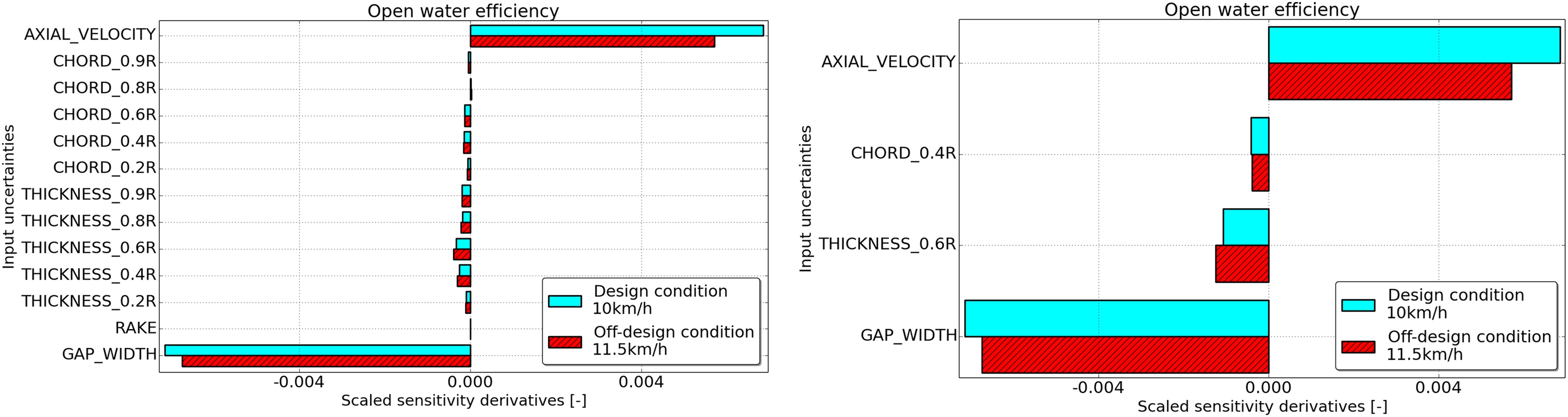
In addition, an operational uncertainty for the ship speed is taken into account in the UQ analysis. An initial UQ study is performed with these 13 uncertainties. Then the scaled sensitivities are analyzed and as a result all chord and thickness uncertainties are merged together, i.e. the change in the shape of the blade profile is controlled by a single section. The rake uncertainty is found negligible for this most stringent tolerance class taken for the study. This reduces the number of uncertainty parameters to 4. As Figure 14 shows, the analysis of the scaled sensitivities with 4 uncertainties are equivalent to those accounting for 13 uncertainties. The reduction by means of scaled sensitivities is therefore valid and the robust design optimization is performed accounting for the remaining 4 uncertainties.
Figure 14.
Scaled sensitivity derivatives of the open water efficiency with respect to the full set of characterized uncertainties (left) and the reduced set of uncertainties (right).
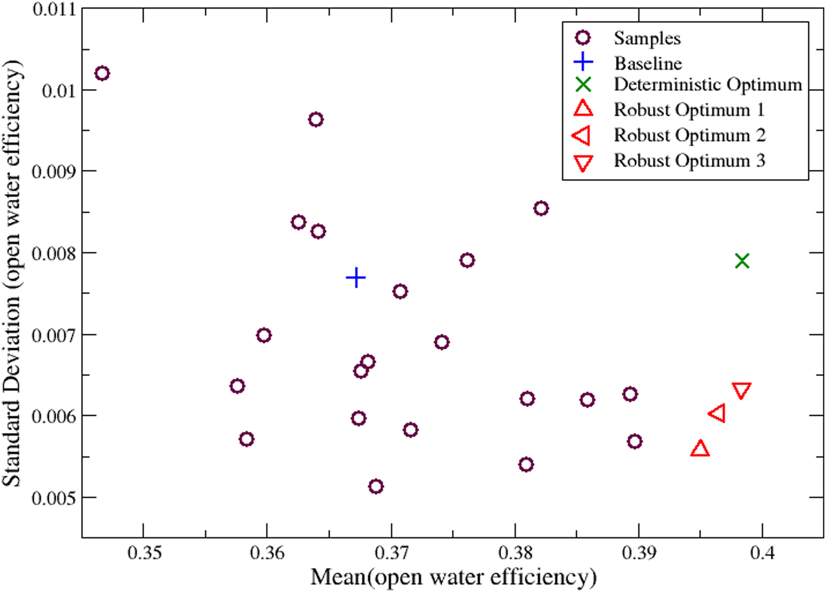
The robust optimization maximizes the mean value of the open water efficiency and simultaneously minimizes the standard deviation of the open water efficiency. Figure 15 shows the resulting Pareto plot, where the standard deviation of the open water efficiency is plotted over the mean value of the open water efficiency. The baseline design is indicated by the “+” symbol. A standard deterministic optimization is performed for reasons of comparison with the robust design optimization. To plot the results of the deterministic optimization in the same diagram a UQ simulation is done on the deterministic optimal geometry. This deterministic optimum is indicated by the “x”. The mean value of the open water efficiency has increased by 8.5%, but the standard deviation has also increased slightly by 2.6%. Three robust optimal designs are shown on the plot by the plain “o”. It is seen that the mean value has increased, but at the same time the standard deviation has decreased. In the example of robust optimal design 3, the mean value has also increased by 8.5%, but the standard deviation has decreased by 17.7%, which means the propeller design is notably more robust with respect to the characterized manufacturing uncertainties and provides at the same time the same mean performance increase.
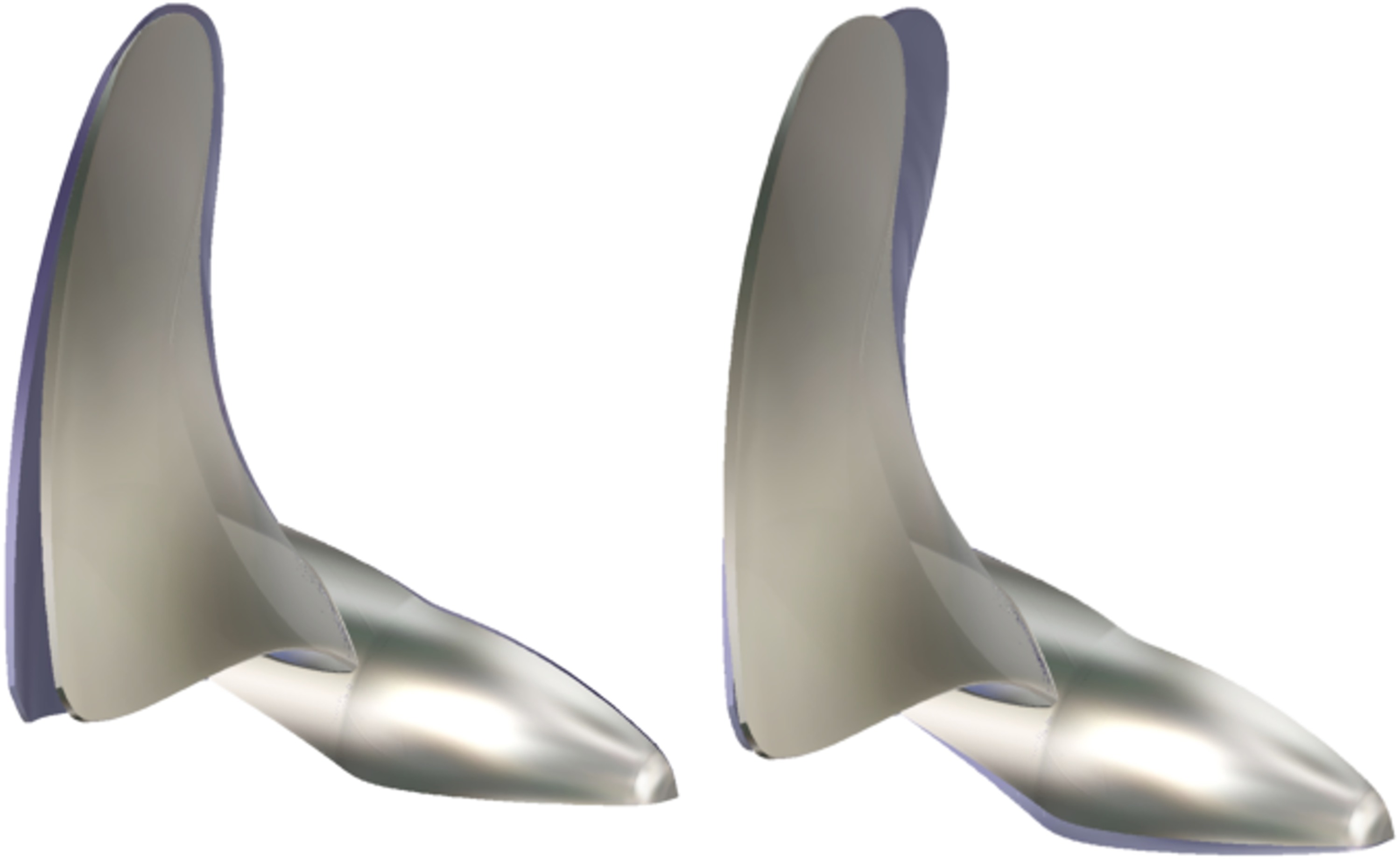
As a last result it is noteworthy that the resulting blade shapes from the standard deterministic and robust design optimization are significantly different, despite the fact that both increase the mean efficiency by the same amount. Figure 16 shows a comparison of the deterministic optimal and robust optimal geometry with the original propeller shapes respectively.
Conclusions
To address the problem of a suitable characterization of manufacturing uncertainties an approach for deriving manufacturing variability from technical tolerancing norms is presented. On top of this method, a virtual sampling method is built and applied and then combined with principal component analysis. This methodology is applied to a high-pressure turbine blade. Propagating uncertainties for the various tolerance classes, it is found that the most stringent class does not bring an advantage in performance stability over the next less stringent class. Exploiting uncertainty quantification methods provides a quantitative assessment of the impact of manufacturing tolerances and as in the presented turbine case could lead to significant cost savings in the manufacturing process, if a less stringent tolerance class can be imposed.
The virtual sampling method is used to run a convergence study on the number of geometries required for the computation of the eigenvalues resulting from the PCA. It is found that 2,000 geometries are needed to converge the computation of the eigenvalues, which is sensibly above the number of geometries that are typically experimentally measured. A sufficiently large sample size is important because the eigenvalues represent the variances of the uncertainties resulting from the PCA and unconverged values could lead to wrong conclusions.
The geometrical influence of the first three eigenmodes obtained is discussed and it is shown that the first and second eigenmode deform the geometry in the order of the span height and chord length of the blade respectively. The third eigenmode is found to have smaller geometrical influence mainly in the region of the blade leading edge. Then UQ simulations are performed for sets of eigenmodes retained and it is shown that adding mode 3 adds significantly to the predicted variance of the isentropic efficiency despite its relatively low geometrical influence. The analysis of scaled sensitivity derivatives confirms the importance of the 3rd eigenmode in this respect. This shows that the geometrical reconstruction accuracy of the deformation modes and reconstruction accuracy of the CFD predictions are not linearly related, which is something that should be kept in mind when truncations are performed on the basis of geometrical variability only.
Finally, the results of an application of the UQ and RDO method used to the robust optimization of a marine propeller are shown. The manufacturing uncertainties are characterized on the basis of the relevant tolerancing norm for marine propellers. Scaled sensitivity derivatives are used to reduce the number of uncertainties before performing a robust design optimization. The robust design optimization maximizes simultaneously the mean value of the open water efficiency and minimizes its standard deviation. It is shown that only a robust optimization formulation can reduce the variability of the performance with respect to the manufacturing uncertainty and that the resulting blade shapes from deterministic and robust optimization are significantly different.