
Introduction
Driven by the demand for highly efficient gas turbines the design methodology of multi-stage compressors has made an enormous progress over the last decades: An example of a classic compressor design conducted manually with throughflow and blade-to-blade analysis is the EEE compressor (Holloway et al., 1982). The compressor consists of different types of airfoils along the stages: special airfoil designs in the front, multi-circular arc thickness distributions in the mid and NACA 65 thickness distributions in the rear. In the 90s numerical optimization emerged in compressor design: Köller et al. (2000) employed direct numerical optimization in combination with the blade-to-blade flow solver MISES to generate a set of optimal airfoil geometries for systematically varying cascade properties. At component level, early work conducting throughflow design optimization includes the studies of Oyama and Liou (2002). Blade-to-blade optimized airfoil sections with a strategy similar to Köller et al. (2000) have been applied to the mid stages of an industrial compressor in (Sieverding et al., 2004). The new blade designs have been evaluated with 3D CFD and measurements. In (Ikeguchi et al. 2012) a 14-stage compressor has been designed based on an automated airfoil optimization system combined with 3D CFD analysis.
During this evolution, the design space for multi-stage compressors increased continuously by allowing more freedom to construct blade shapes. In addition, the state-of-the-art moved away from the idea of stacking 2D designed airfoils to optimizing the whole blade geometry with 3D CFD in order to control end wall flow. Nevertheless, throughflow design remains an important step on the way to a successful compressor design as it enables the designer to rapidly explore the design space. However, the way from a throughflow design to a 3D compressor geometry can be cumbersome. Accordingly, a close coupling between throughflow and blade-to-blade design can speed up the product development cycle significantly. The overall goal of this work is to examine a method that generates a full 3D compressor geometry with blade-to-blade optimized airfoils on the basis of a throughflow design.
This is realized by using the airfoil family presented in (Schnoes and Nicke, 2017b). It was generated by filling a database with optimized airfoil shapes similar to the work of Köller et al. (2000). On this basis, a functional relation between a set of design requirements and corresponding optimal airfoil shape was derived. The idea was to produce a highly versatile airfoil family that covers most applications in the core compression system of aircraft engines and stationary gas turbines. In this work, strategies to describe the performance of the new airfoils are presented and are implemented into a throughflow code. For a full assessment of the new airfoils, these methods are applied to an existing heavy-duty gas turbine compressor test rig. The performance is compared between throughflow and 3D CFD. Afterwards, the design is optimized to study further upgrade options for the compressor.
Methodology
This section gives details about the database of optimal airfoils that is used for compressor design. The focus lies on the connection of the airfoil family to throughflow calculation and blade geometry generation. More details about the airfoil database can be found in (Schnoes and Nicke, 2017a,b).
Database of optimal airfoils
The airfoil family in this work is generated based on a parametric study on the geometry of optimal airfoils for a variation in geometric cascade parameters and design point operation conditions. These parameters, denoted as “design requirements”, form a seven dimensional requirement space: stagger angle
In classic airfoil families a variation of flow turning is achieved by modifying the blade camber. For this work, the design point diffusion factor is varied as no prior knowledge is available on the attainable flow turning of the optimized airfoil shapes. It seems that the design inflow angle is missing in the requirements, but a variation of the stagger angle makes it is possible to find an appropriate airfoil design for different inflows.
A lower and upper bound is chosen for each design requirement with values given in Table 1. This box-constrained requirement space contains large regions that do not occur in compressor design or are infeasible. For example, it includes airfoils with low stagger angles at supersonic inlet Mach numbers. This scenario has high axial Mach numbers that might become supersonic. Accordingly, additional constraints are imposed to ensure that a feasible airfoil exists for each set of requirements. For the given example, the region is blanked by introducing a constraint connecting stagger angle and inlet Mach number.
Table 1.
Upper and lower limits for each design requirement.
| Min | 0.35 | 0.5 | 110.0° | 1.5% | 0.35 | 1.0 | |
| Max | 1.20 | 1.2 | 147.5° | 8.5% | 0.55 | 1.2 |
In the next step, a large number of airfoils is generated based on a design strategy for compressor airfoils at discrete points in the requirement space. The strategy employs numerical optimization and evaluates each candidate airfoil by computing the loss characteristic around the design point with MISES (Drela and Youngren, 1998). The target is to find airfoil shapes that have low losses and ensure stable operation over wide incidence ranges. Around 2000 airfoils have been designed automatically with this strategy. In the end, many requirements for the design of multi-stage axial compressors are covered by this database: from transonic front to subsonic rear stages, from thick hub to slender tip blade sections. In (Schnoes and Nicke, 2017b) the methodology is validated by analyzing the performance of two transonic cascades with RANS simulations. For two further subsonic cases, new airfoils are compared to a Controlled Diffusion Airfoil (CDA) and a state-of-the-art stationary gas turbine airfoil.
Estimation of optimal airfoil shape
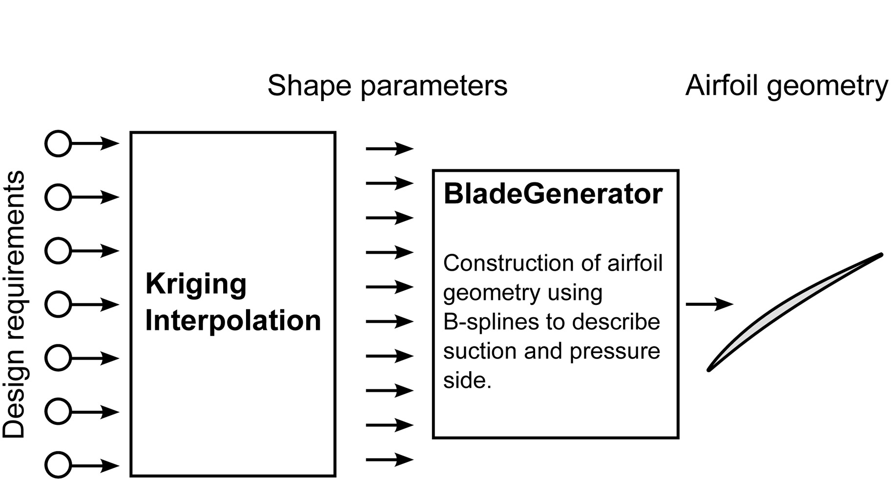
At this point, optimal airfoils are defined at discrete points in the requirement space. On this basis, interpolation and approximation routines can be used to create airfoils for new requirement sets. It would be possible to directly relate design requirements and airfoil geometry. Instead, a detour is taken: at first, shape parameters of the parametric blade definition tool “BladeGenerator” are predicted. Afterwards, the actual airfoil geometry is created by executing the program, as shown in Figure 1. The detour is taken to stay in line with an established design work flow. Furthermore, “BladeGenerator” can directly stack the interpolated airfoils to a 3D blade. The interpolation problem comes down to multivariate interpolation of scattered data on an irregular grid. Multiple interpolation methods have been compared and finally Kriging (Matheron, 1963) is chosen.
Estimation of loss and deviation
When it comes to throughflow calculation, an estimation of 2D cascade loss and deviation is required instead of airfoil geometry. Typically, empirical correlations are used, that are calibrated by data from wind tunnel tests. In previous work (Schnoes and Nicke, 2015), a method is proposed to calibrate loss and deviation correlations automatically against blade-to-blade simulations with MISES. The procedure is suited to describe custom tailored airfoils that are not covered by classic correlations. To understand the way correlations are calibrated, a short look at the prediction of the deviation angle δ is taken. The deviation angle is the difference between outflow angle and the blade metal angle at the trailing edge. It can be estimated with the well-known Carter’s deviation rule (Carter, 1950). The following is a modified version including a
where m is an empirical function of blade stagger and
Figure 2.
Correlation framework to estimate 2D cascade loss and deviation based on a set of empirical calibration parameters.
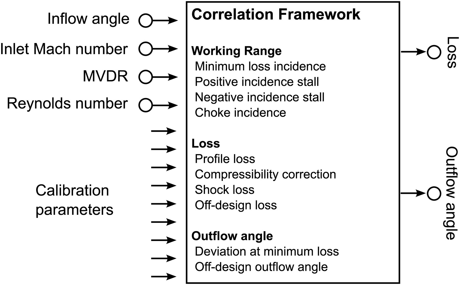
This set of correlations can be fitted to a specific airfoil geometry with a “direct” method: At first, a set of 40 loss and deviation characteristics is computed with MISES for a variation in inlet Mach number, Reynolds number and MVDR. Secondly, calibration parameters for loss and deviation models are determined by solving a set of nonlinear least-squares problems. This mode is used to create throughflow models of existing compressors by calibrating separate models on multiple blade sections and interpolating between them.
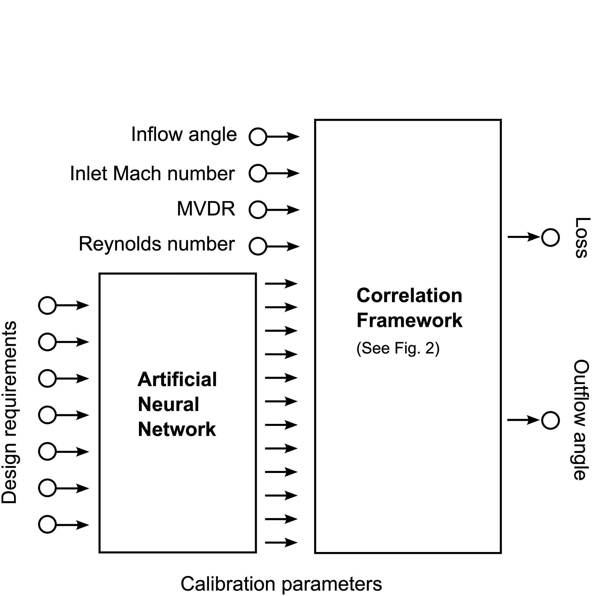
For the design of multi-stage machinery, the direct calibration method is impractical due to the fact that new airfoil geometries have to be sampled with MISES. A faster method is employed for the new airfoil family: For a given set of design requirements, a neural network predicts the calibration parameters of the loss and deviation model. Figure 3 gives a schematic view for this method. The artificial neural network is a simple multilayer perceptron with only one hidden layer and sigmoid activation functions. A low number of weights in combination with L2 regularization results in a high degree of generalization. The training set consists of the above mentioned 2,000 optimized airfoils. A validation set has been generated by interpolating 1,000 airfoil geometries at random locations in the requirement space. The performance of each airfoil in both sets is sampled with 40 loss and deviation characteristics. All in all, this gives over one million MISES computations. The neural network is trained together with the correlation framework with the objective to find weights that result in a minimum approximation error of loss and outflow angle. The overall prediction scheme is included in the throughflow code.
Figure 3.
Estimation of loss and deviation for database airfoils based on a neural network in combination with the correlations presented in Figure 2.
Finding corresponding airfoils
When deploying the new airfoils it is a common task to search for a database airfoil that corresponds to an existing airfoil. In other words, the problem is to find the design requirements for a database airfoil with a working range that possibly surrounds the working range of the baseline airfoil while having a similar outflow angle. In this case, pitch-chord ratio and profile area can be taken from the baseline. Additionally, a design point has to be specified by providing the properties inlet Mach number, Reynolds number and streamtube contraction. This leaves stagger angle and design point diffusion factor to be determined. These can be specified by a two parameter optimization based on a comparison of the directly fitted loss and deviation correlation of the existing airfoil (see Figure 2) and the performance prediction of the airfoil family (see Figure 3). On this basis, after the correlation of the baseline airfoil is determined with the methods from above, a corresponding airfoil can be found extremely fast.
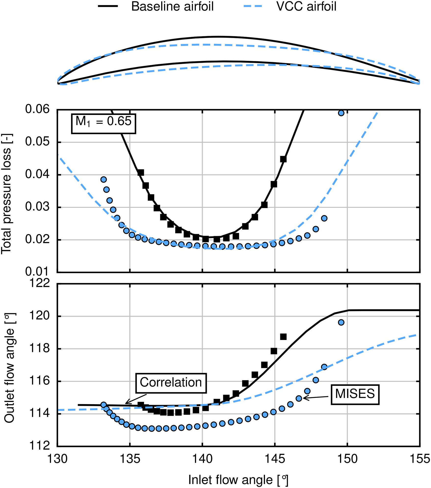
An example is given in Figure 4 where an existing subsonic stator airfoil and a corresponding interpolated airfoil are compared. The performance of the airfoils is evaluated by blade to-blade computations with MISES. Furthermore, the directly computed correlation for the baseline airfoil is given and compared to the estimated correlation for the new airfoil. For the baseline geometry an excellent agreement between the correlation and the blade-to-blade computations can be observed. It is noteworthy that the extrapolation behavior of the outflow angle at high incidences flattens and converges to a constant value. This presumption is made to achieve a high stability in throughflow computations. Regarding the correlation prediction of the database airfoil, the correlation shows a significantly larger working range with slightly lower losses and a similar outflow angle. The MISES calculations confirm the increase in working range but the increment in losses is steeper for both positive and negative incidence stall than predicted by the correlation. The most severe error occurs for the outflow angle: a shift of about 1.3° can be observed. At this point it is not clear if the error is caused by the prediction of geometry or correlation. A higher number of optimized airfoils might decrease this fitting error. All in all, the performance of the new airfoil is superior and the approximation error in the performance estimation is acceptable.
Figure 4.
Baseline stator airfoil and corresponding interpolated airfoil. Comparison of results from correlation (Figure 3) and MISES.
Compressor test rig
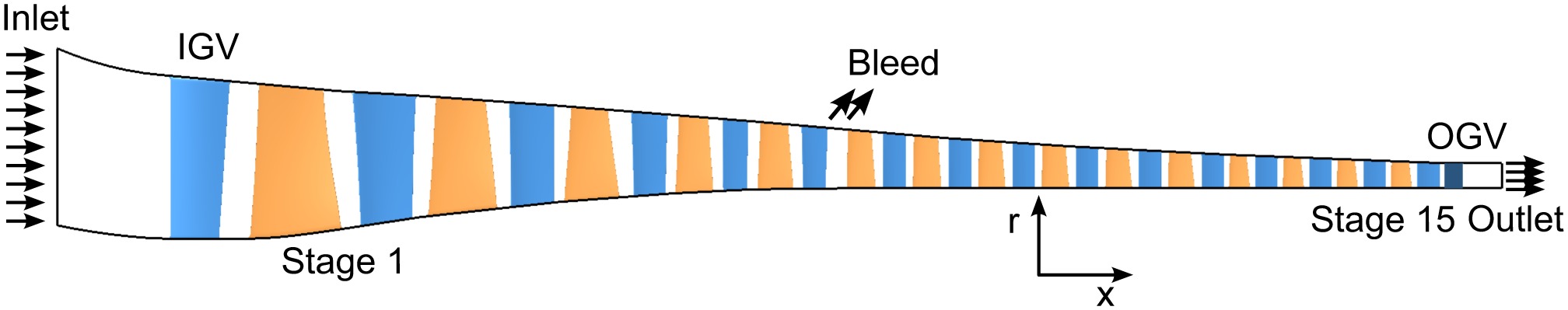
The database airfoils are now implemented into the 15-stage compressor test rig shown in Figure 5. The rig was tested in 1994 by MTU Aero Engines (Hansen and Kappis, 2001). It is a geometrically scaled variant of a heavy-duty gas turbine compressor. The blades are constructed from CDA sections. An inlet and an outlet guide vane accompany the 15 stages and a bleed port is situated after stage 5 where 2.5% of the inlet mass flow is extracted. For the studies at hand, all stator rows are modeled as cantilevered blades with hub clearances. Relative corrected rotational speeds between 90% and 105% are examined while the variable guide vanes remain fully opened. This covers an operation range from weak grid on a hot day up to cold day.
In the following, the baseline configuration of the compressor is compared to a version that uses airfoils from the presented database. The new variant is denoted as “VCC blading”.
Throughflow setup
The throughflow calculations are performed with the streamline curvature (SLC) program ACDC developed at DLR (Schmitz et al., 2012). The code uses the loss and deviation correlations presented above. Airfoils are represented by their correlation parameters which are prescribed on multiple radial heights for each blade row. While streamlines move up and down during the solution procedure, calibration parameters are interpolated to the streamlines based on the current radial height in order to evaluate loss and outflow angle.
In order to create a throughflow model of the baseline configuration, four airfoil geometries are extracted from each rotor and three airfoils from each stator. For every airfoil, a design point is extracted from a 3D CFD simulation of the compressor. The resulting 2D cascades are sampled with MISES and loss and deviation correlations are fitted with the direct calibration method described above. During the sampling procedure almost 60,000 MISES computations are launched. On current hardware this takes several hours.
For each baseline airfoil, a corresponding database airfoil can be found automatically with the presented methods. In this case, the throughflow code outputs all the information necessary to stack the blades and generate the 3D geometry of the compressor.
In addition to 2D cascade loss and deviation, correlations for 3D flow phenomena are included in the blade row model: The correlations outlined in Grieb et al. (1975) are implemented to estimate secondary losses. Tip clearance losses are computed with correlations based on the work of Denton and Cumpsty (1993) and Banjac et al. (2015). The effect of tip clearance flow on deviation is accounted for by the deviation model of Lakshminarayana (1970). 3D deviation and losses are distributed over the blade span by functions adopted from Roberts et al. (1986). The overall level of losses of the tip clearance and of the secondary flow model is adjusted manually to receive a design point efficiency that is close to the RANS results of the baseline. Span-wise mixing is accounted for by a turbulent diffusion process based on the work of Gallimore (1986). The stability of the compressor is evaluated with the semi-empirical method proposed by Koch (1981).
Steady-state RANS setup
Throughflow results are compared to simulations carried out with the 3D CFD solver TRACE (Kügeler et al., 2008; Becker et al., 2010). TRACE is developed at DLR for turbomachinery application. Steady-state RANS simulations with a Wilcox k-
Results
The compressor map of the baseline design and of the VCC bladed version comparing 3D CFD as well as through flow is given in Figure 6. At nominal speed, the 3D CFD results of both versions match very well in terms of mass flow rate and total pressure ratio. A slight increase in design point polytropic efficiency of 0.27% is accomplished with the new airfoils. The other speed lines are in a good agreement as well.
Figure 6.
Performance map comparing baseline design and VCC blading for 90% up to 105% relative speed.
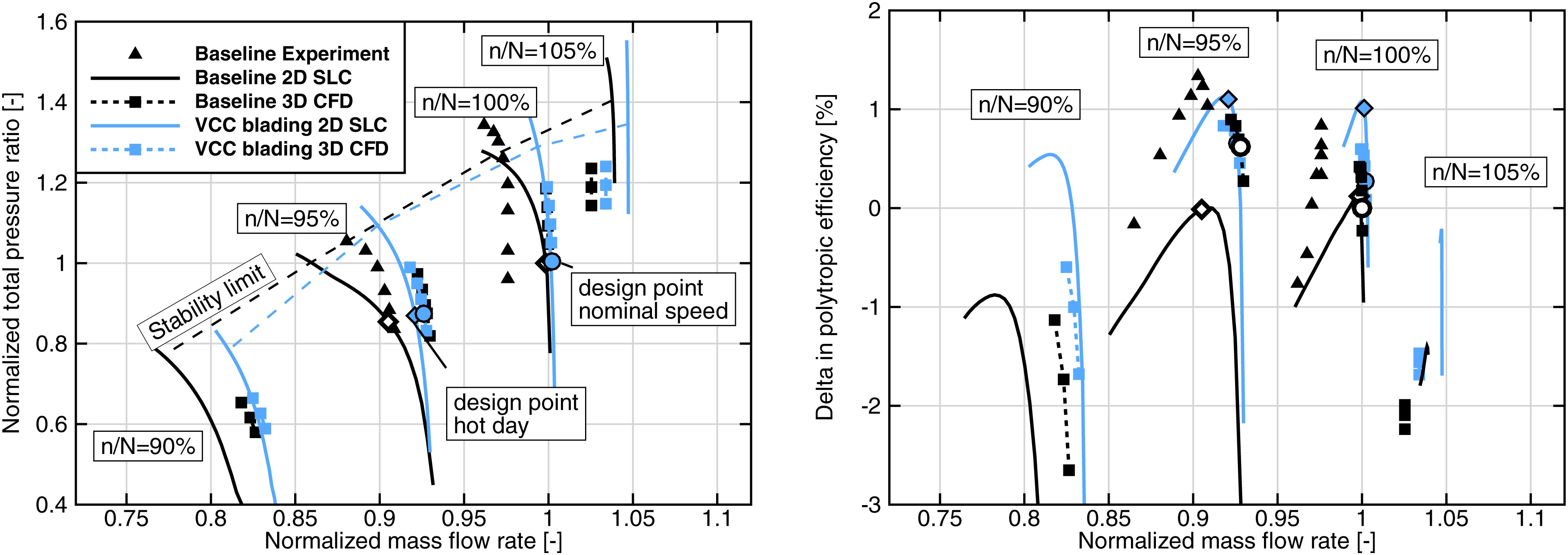
Regarding the throughflow results, significant differences between both compressor designs can be observed. An increase in design point efficiency of 0.89% is predicted at 100% speed, which is not reflected by 3D CFD. Additionally, the speed lines of the throughflow simulations of the baseline design show a different characteristic with a larger drop in mass flow rate close to the stability limit.
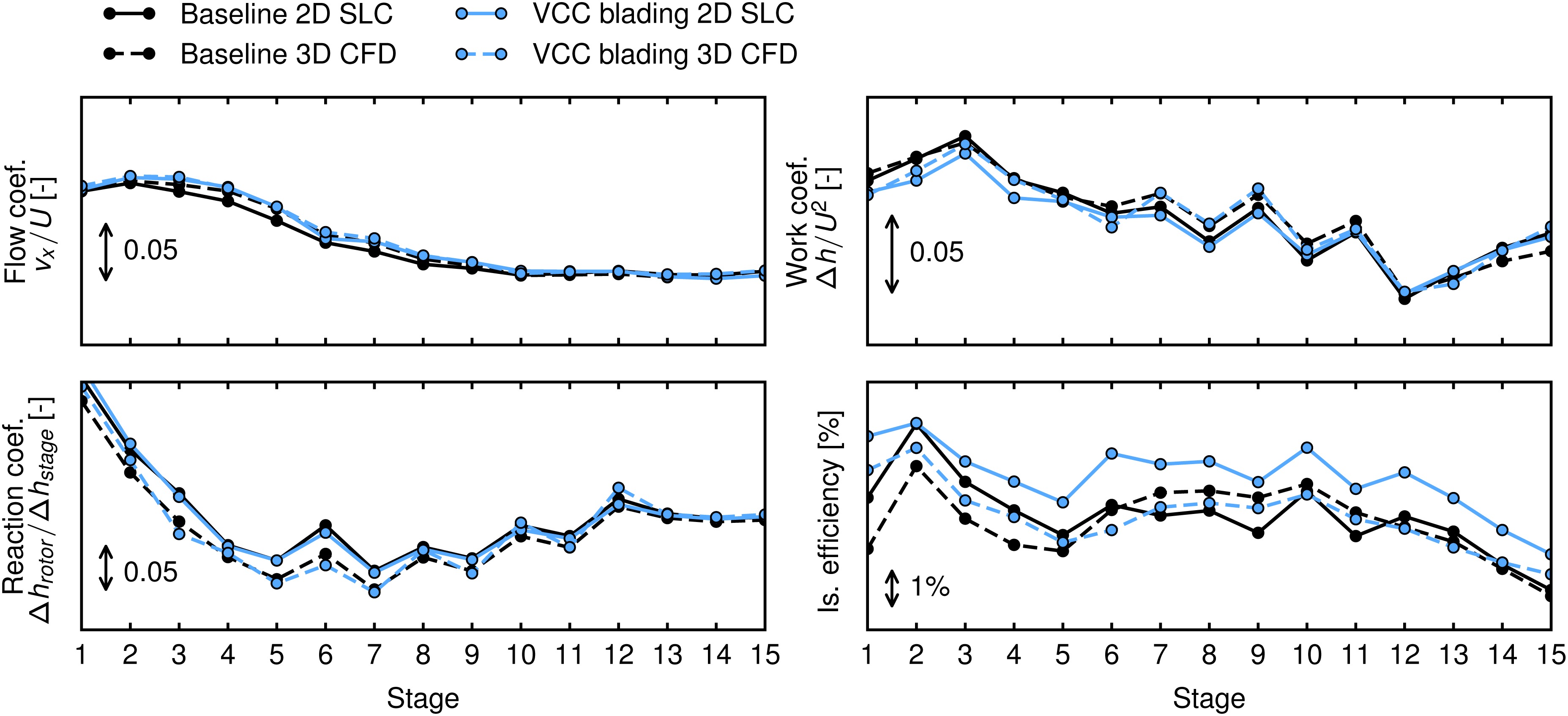
Figure 7 examines the design point on the 100% speed line more closely: for each stage the flow coefficient, the work coefficient and the isentropic efficiency is given. Both flow and work coefficient match well for 3D CFD and throughflow for both compressor configurations. Only a slight axial redistribution of load can be observed between the VCC blading and the baseline design. Regarding the isentropic efficiencies, both 3D CFD and throughflow share the following trends: a very efficient second stage, after which the efficiency decreases up to stage five. After the bleed, the efficiencies recover, before dropping again over the last four stages. The most obvious difference is that, as already seen in the compressor map, throughflow computations significantly over-predict the efficiencies for the VCC blading. Comparing both 3D CFD results, gains in efficiency up to 1.91% are observed for the first five stages. For the mid stages, VCC blades have a slightly lower efficiency with a maximum decrease of 0.49% at stage 6. The rear stages are very similar again. Generally, the new airfoils seem to perform well for transonic stages, but a slight increment in losses can be observed for the majority of the subsonic stages. This is in contrast to the results from 2D cascade analysis which promised a superior performance over CDA blading throughout a wide range of inlet Mach numbers.
Figure 7.
Flow coefficient, work coefficient, reaction coefficient and isentropic efficiency for each stage comparing baseline and VCC blading for the design point at nominal speed.
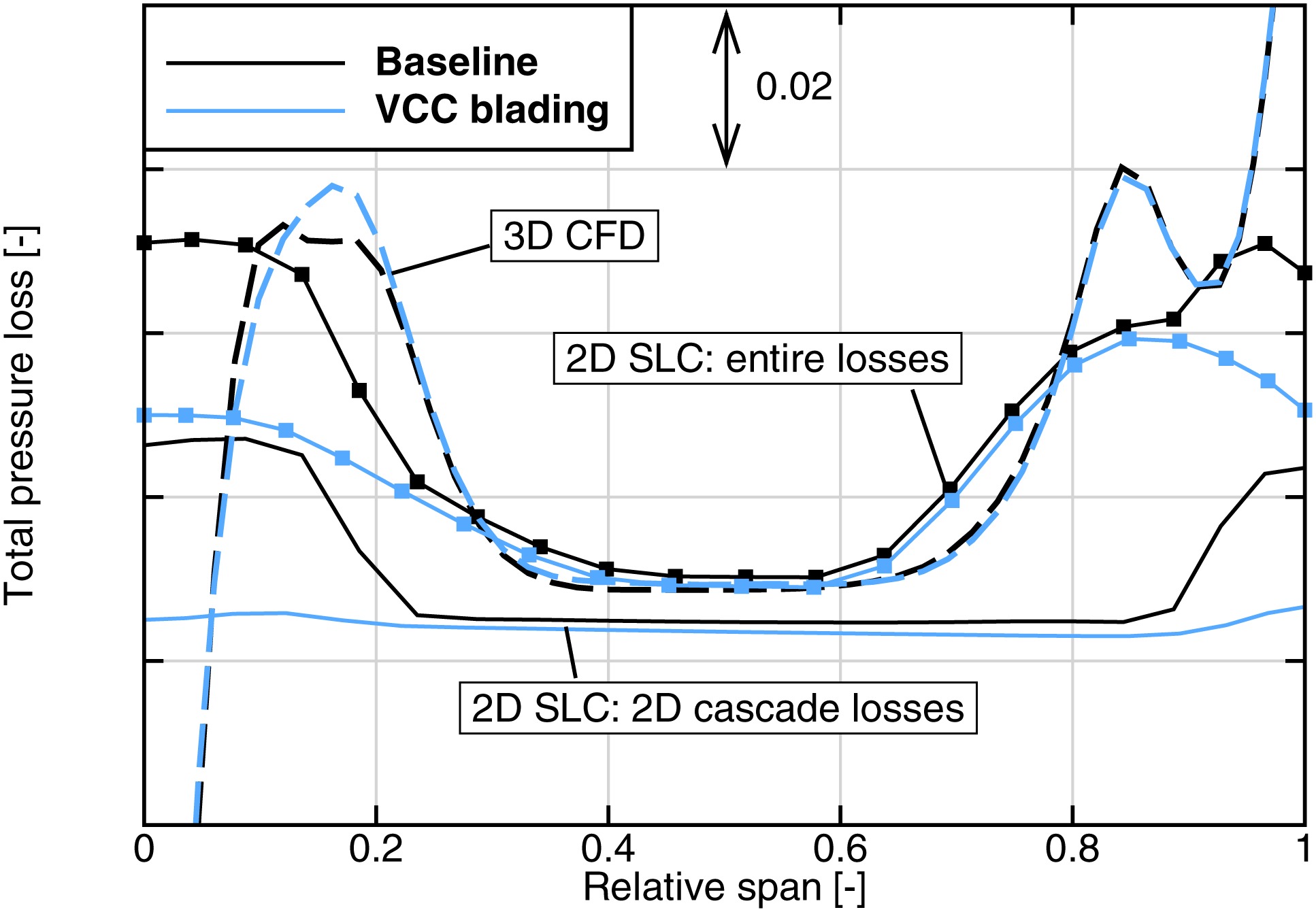
The reason for the difference between the throughflow solutions of baseline and VCC blading can be found in the estimation of blade losses. Figure 8 shows the losses of the 2D cascade correlations and of the secondary flow correlations comparing them to the losses from 3D CFD for rotor 10 in the design point at nominal speed. Regarding the baseline design, the 2D cascade losses show a substantial increment close to the end walls due to flow incidence. Having in mind that the new airfoil family has higher working ranges in 2D (see Figure 4), profile correlations predict only a slight loss increment in the end wall region. And although both designs show different working ranges on a 2D cascade level, the actual losses computed with 3D CFD are similar. Accordingly, 3D flow dominates the end wall regions and the breakdown of losses into 2D cascade losses and 3D secondary flow losses is an idealization. Thus, a careful calibration between all involved correlations is important for accurate throughflow design. Here, a different calibration of the secondary flow model between database and CDA blading is an option to improve results. It becomes evident as well that the only difference in 3D CFD between both designs is found in the slight difference of secondary flow at the hub end wall.
Figure 8.
Loss contributions in throughflow calculation in comparison to 3D CFD results for rotor 10 in the design point at nominal speed.
For further validation of MISES to design airfoils, the isentropic Mach number distribution of two blade sections is compared to the 3D CFD results. At first, a section of the transonic first rotor at 73% relative span is analyzed in Figure 9. The operating point is at design condition on the 100% speed line. The shock system of the baseline design consists of a detached bow shock that hits the suction side of the adjacent blade at 50% chord. Further downstream at 75% chord on the suction side a passage shock follows. Accordingly, the baseline design is choked. The new airfoil design accelerates to higher Mach numbers on the suction side, but the deceleration occurs in a single shock. By avoiding choke, and the corresponding losses from the passage shock, the efficiency of the first stage increases significantly as already seen in Figure 7. All in all, MISES and 3D CFD are in good accordance.
Figure 9.
Isentropic Mach number distribution comparing 3D CFD and 2D blade-to-blade results for baseline and VCC blading for rotor 1 at at relative span of 73% for the design point at nominal speed.
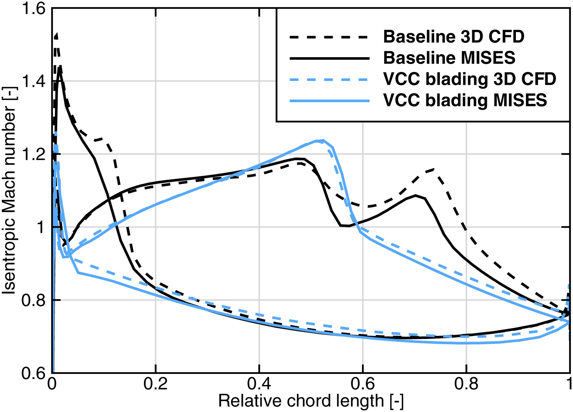
The majority of the stages is subsonic, picking one example, a closer look at the mid-section of stator 10 is taken in Figure 10. For this section, a near stall operating point with 20% increased back pressure from the design point at nominal speed is selected. The same operating point and stage is analyzed for flow separation below. The maximum suction side Mach number increases for the new airfoil design and the position of the maximum moves upstream. After a first strong deceleration, there is hardly any change in velocity between 50% and 80% chord. Afterwards the flow decelerates to its final value at the rear. Again, the isentropic Mach number distribution of the blade-to-blade design can be confirmed with 3D CFD.
Figure 10.
Isentropic Mach number distribution comparing 3D CFD and 2D blade-to-blade results for baseline and VCC blading for stator 10 at mid span for a near stall operating point at nominal speed.

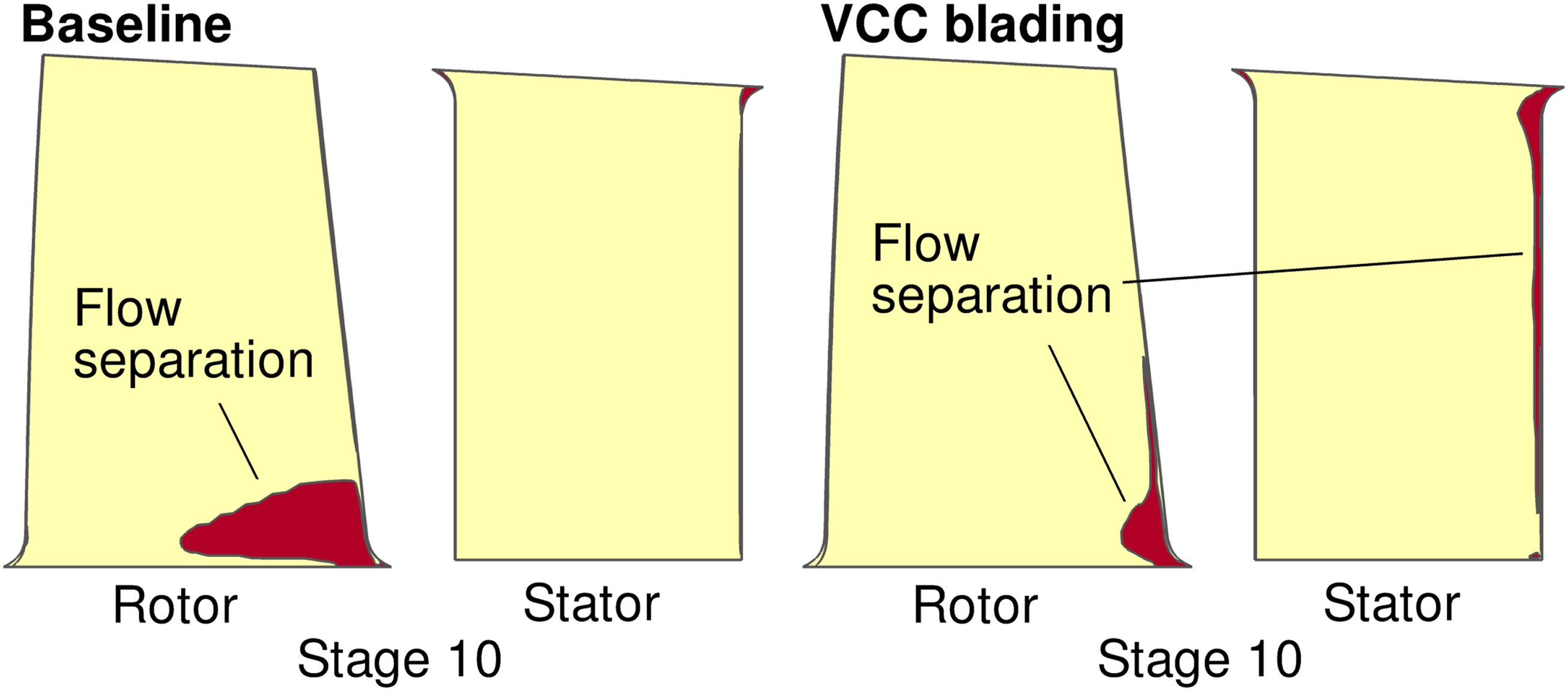
At last, a closer look at the failure mode of both compressor configurations is taken. Examining the wall shear stress at the near stall operating point at nominal speed, the largest patches of flow separation can be found at rotor 10 as visualized in Figure 11. The baseline design shows a large corner stall that reaches almost to mid chord. The patch is less mature for the VCC version, but a small separation stretches along the trailing edge of rotor and stator. This flow separation is induced by the strong rear loading that was discussed in Figure 10.
Figure 11.
Visualization of flow separation based on wall shear stress for the suction sides of rotor and stator of stage 10 at a near stall operating point at nominal speed. Red indicates a negative wall shear stress and thus a separated boundary layer.
All in all, the new airfoils have proven their value in a 3D setup and show potential for transonic stages. For subsonic mid and rear stages, where secondary flow is the dominant source of losses, the strong rear loading of the airfoils seems to limit the performance by causing slightly increased secondary flow.
Optimization studies
In the following part upgrade studies are conducted for the test compressor. The objective is to increase the efficiency as well as the mass flow rate in order to improve the power output of the stationary gas turbine. The basic engine architecture is not supposed to be changed. Correspondingly, the flow path as well as the blade positions and the blade counts are not modified. Instead, new airfoils are used to stack the blades. For the studies at hand the optimization suite AutoOpti (Aulich et al., 2014; Voss et al., 2014) is used. During the optimization, the compressor performance is evaluated with throughflow simulations. Afterwards, three configurations from the Pareto-front are selected and their performance map is evaluated with throughflow and 3D CFD.
Optimization setup
In contrast to the VCC bladed version of the compressor, new design requirements are assigned to each blade section during the optimization. A subset of the design requirements can be determined during the throughflow computation of the design point: in each iteration of the solver, inlet Mach number, streamtube contraction and Reynolds number are extracted from the current flow solution. Accordingly, the design point throughflow calculation fixes these parameters for the off-design points. The design pitch-chord ratio is defined by the blade count, the axial chord and the stagger angle. The span-wise evolution of profile area is left untouched. A more detailed analysis of structure mechanics is disregarded in this study. This leaves only the design point diffusion factor and the stagger angle as free optimization parameters for each blade section.
As the rotors are continued to be stacked by four airfoils and the stators by three airfoils, all 15 stages together yield 210 parameters. An optimization with this number of parameters is very expensive. This contradicts the idea of doing fast design studies with throughflow computations. Accordingly, the number of design parameters has been reduced by applying 2D splines in axial and radial direction that add deltas to the existing compressor. Four 2D spline interpolations are used: for both stagger angle and design diffusion factor, independently for rotors and stators. The optimization parameters are formed by the control points of the 2D splines. With five control points along the axial direction, and four (three) control points along the span for rotors (stators) the number of design parameters is reduced to 70. The resulting optimization runs over night on a work station with current hardware. This is in the same order of magnitude as the computational expense to simulate one operating point with 3D CFD. In the presented case, it was found that an optimization with 210 parameters does not offer significantly more improvements over the parameterizations with 70 degrees of freedom. It has been tested as well to include the blade counts as design parameters, but resulting compressors had severe issues with stability when computing with 3D CFD. The authors assume that the implemented secondary flow models as well as the stability criterion by Koch do not offer enough fidelity to describe all effects when freely modifying the blade geometries.
For each compressor configuration six operating points are computed in the optimization: two design operating points at 95% and 100% speed and four near stall operating points at 90%, 95%, 100% and 105% speed. Since the mass flow rate of the machine is modified, the equilibrium with the turbine has to be guaranteed. This can be done by increasing the compressor design point total pressure ratio proportional to the mass flow rate. Then, for the assumption of a constant combustion pressure loss, a constant turbine inlet stagnation temperature and an overcritical turbine, the corrected turbine inlet mass flow does not change and continuity is guaranteed (Saravanamuttoo et al., 2009). The near stall operating points are determined by multiplying the outlet pressure of the design operating points by user specified constant values. To attain the desired operating points, PID controllers are implemented in both the throughflow as well as the 3D CFD code.
Two objectives are of interest: increasing the isentropic efficiency as well as the mass flow rate. In order to have an improved performance over a wide operating range, the objective functions are defined as an arithmetic average of the values at the two design operating points.
In order to ensure stable operation, constraints are introduced for the Koch stall criterion at the four near stall operating points. In each point, the stability is not allowed to decrease in comparison to the baseline design. It proofed to be very important to include all four near stall points into the stability constraint as different stages fail depending on the rotational speed. Additionally, the design requirements of each blade section are constrained to the requirement space. This gives a lower and upper bound for the stagger angle.
Results
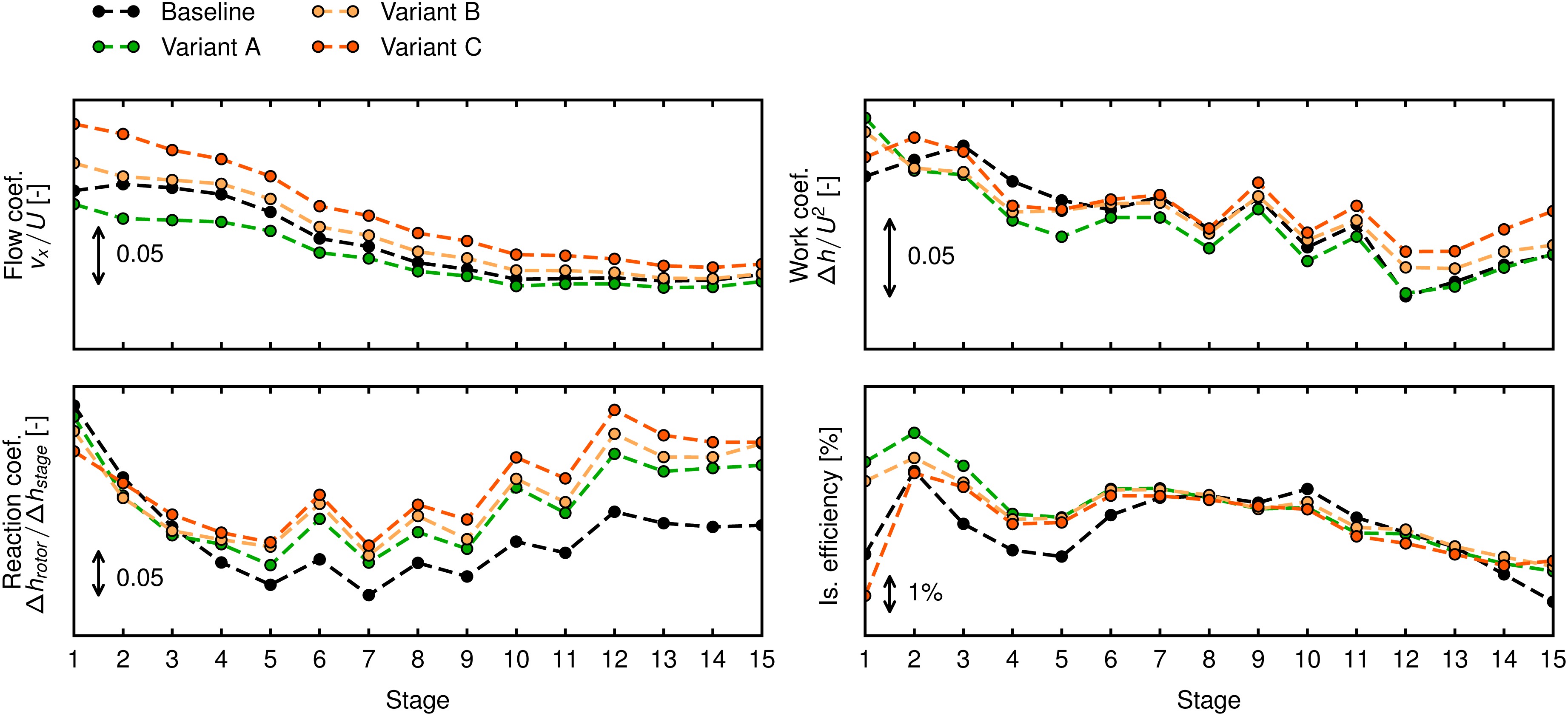
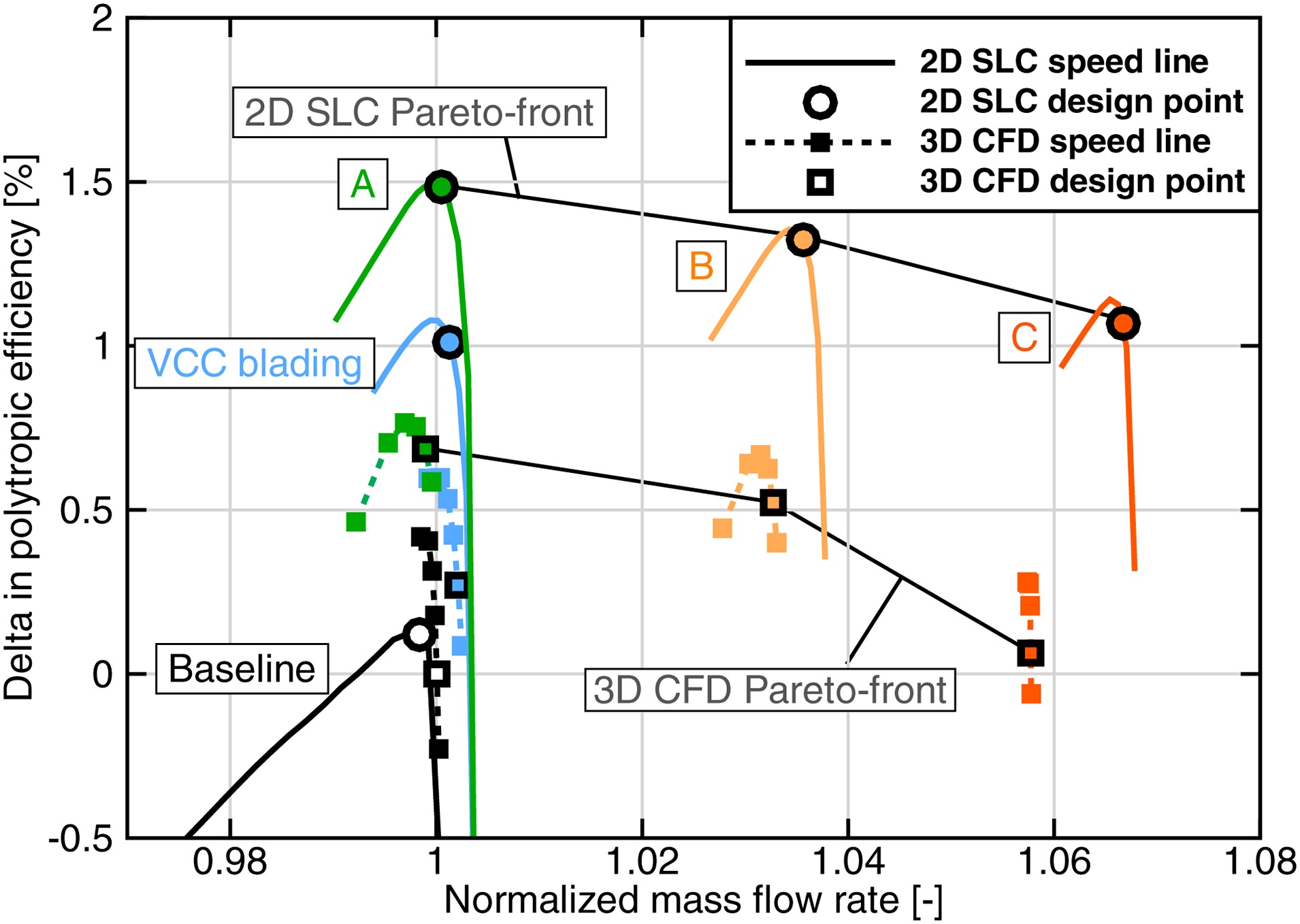
During the optimization process 4,300 compressor configurations have been evaluated. From the resulting Pareto-front three geometries are selected, denoted in the following as variant A, B and C. Figure 12 shows the 100% speed lines for the optimized configurations in comparison to baseline and VCC blading. Both throughflow results as well as 3D CFD results are given. Regarding the 3D CFD design points, configuration A has the highest polytropic efficiency with an increment of 0.69% at a mass flow rate comparable to the baseline design. Configuration C achieves an increase in mass flow rate by 5.8% at an efficiency comparable to the baseline design. Configuration B shows a good trade-off between design A and C with a 3.3% higher mass flow rate and a gain in efficiency of 0.52%. The shift between throughflow and 3D CFD increases from the VCC bladed version to the optimized versions, with higher errors for the configurations at higher mass flows. A closer look at the stage characteristics of the 3D CFD results of the design points at nominal speed reveals more details (Figure 13). Regarding the flow coefficient, configuration B and C have higher values than the baseline design. This is obvious as the flow rate increased while having the same flow path. Furthermore, a redistribution of the work along the compressor stages can be observed: All of the optimized versions show an increase in load on the front stage in comparison to the baseline design. For stages 3–8, there is a trend to have a lower work coefficient. This has to be balanced by the rear stages which provide higher work input. The reaction coefficient is larger in comparison to the baseline design for all stages after stage three. This is reflected in the modifications of the stagger angles: in average the stagger increases slightly for the rotors and decreases for the stators. This design choice is probably grounded in the fact that the clearances are higher in the stators than in the rotors. Looking at the efficiencies, gains are achieved in the first six stages. Except design C: it has a front stage with a lower efficiency than the baseline design. For this design, the first rotor is already choking in the design point due to the high mass flow rate. Between stages 9 and 13 the efficiency drops slightly in comparison to the baseline design.
Figure 13.
Flow coefficient, work coefficient, reaction coefficient and isentropic efficiency for each stage comparing optimized versions to baseline design for 100% speed design point (3D CFD).
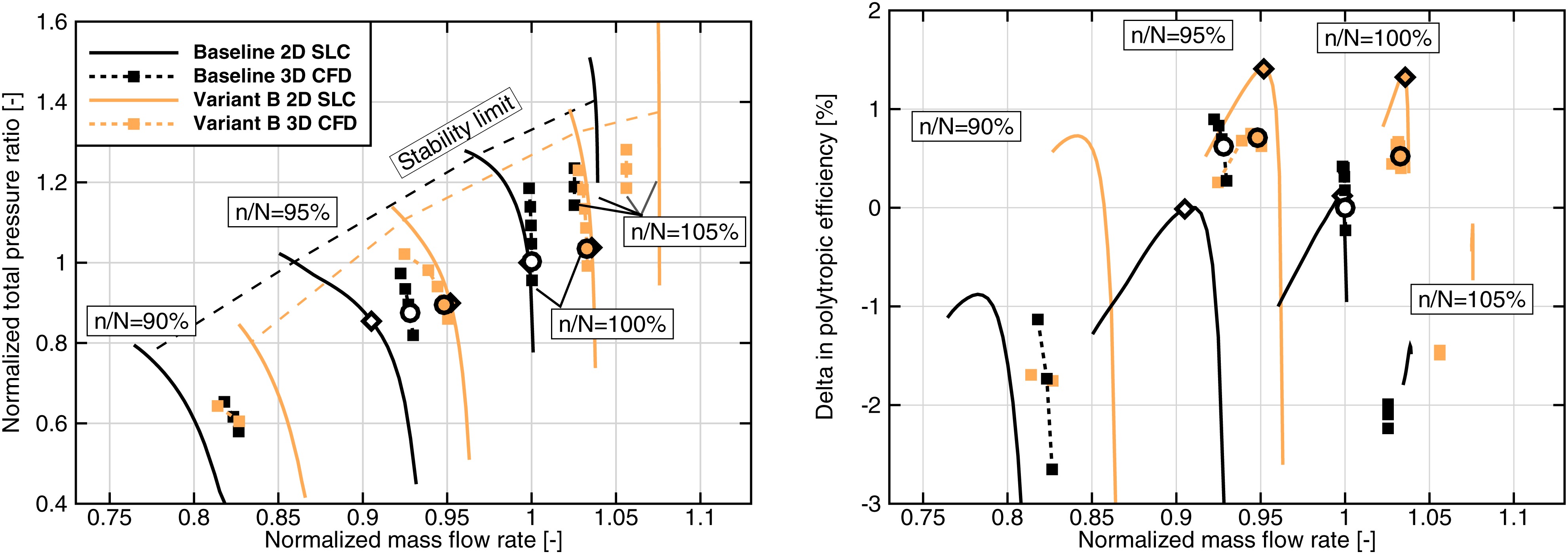
Since variant B offers an interesting tradeoff between efficiency and mass flow rate, the design is analyzed in more detail. Figure 14 gives the performance map for the baseline design and variant B. Most notably the 100% speed line of variant B has a higher mass flow rate than the 105% speed line of the baseline design. The stability margins for both 3D CFD and throughflow are comparable for both designs. The gains in mass flow rate and efficiency become smaller for lower speeds. At 95% speed, the efficiency in the design point is comparable between both versions. For 90% speed, 3D CFD no longer shows an increase in mass flow rate, although throughflow predicts an improvement.
Figure 14.
Performance map comparing baseline design and variant B for 90% up to 105% relative speed.
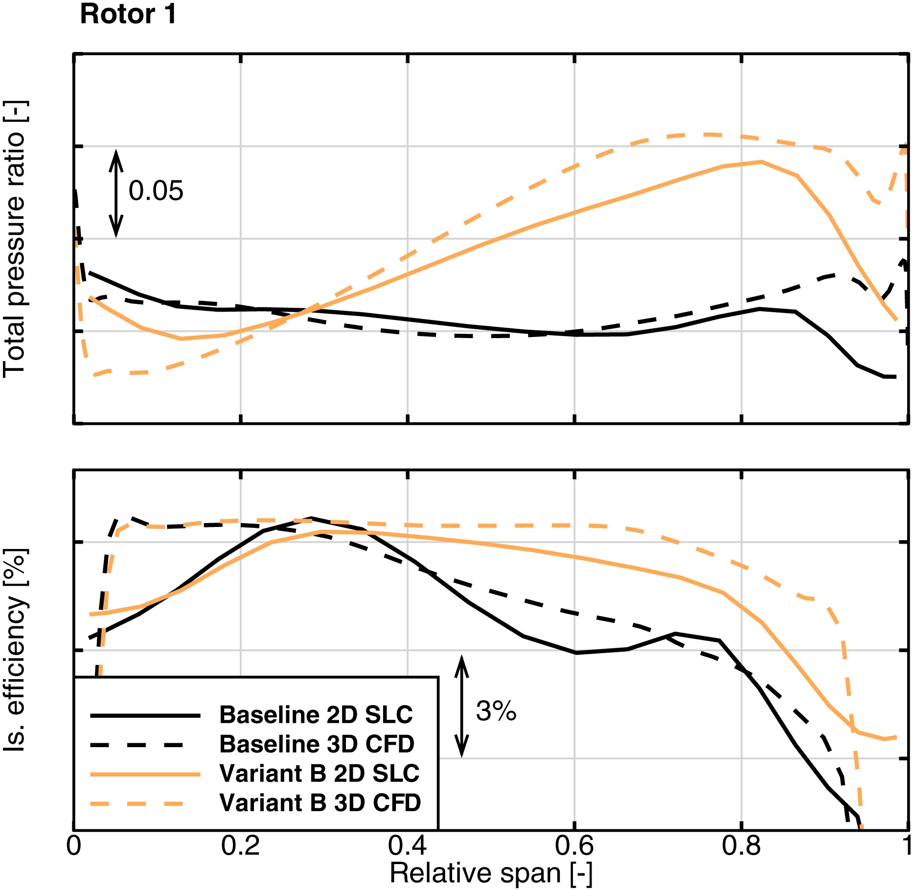
The most obvious changes occur in stage 1, for this reason a closer look at the new rotor design is taken. Figure 15 depicts the span-wise distribution of total pressure ratio and isentropic efficiency of the blade row for configurations baseline and B. The blade row provides significantly more total pressure starting from 25% radial height. The total pressure ratio increases from hub to tip for the new version in comparison to the baseline that has a balanced distribution. At the same time, the efficiency improves in the upper half. At 80% radial height an improvement of 2.9% is achieved regarding 3D CFD. Throughflow estimates an improvement of 1.7%. All in all, 3D CFD confirms many qualitative trends, but the quantitative results are different.
Conclusion
The major result of this work is a novel airfoil family that can be used in the design of multi-stage compressors to construct transonic front stages as well as subsonic rear stages. The new airfoils are part of a work flow that spans from throughflow to 3D CFD.
The performance of the airfoil family is demonstrated on a 15-stage test compressor. For transonic stages, the new airfoils show a substantial increase in efficiency. For subsonic stages, blade-to-blade computations promised improvements over CD airfoils. In the end, the mid and rear stages of the test compressor are dominated by secondary flow, thus the performance turned out to be similar to CDA blading with slightly better efficiencies for CDA and slightly increased stability for the new airfoils.
Afterwards, the compressor is redesigned in a throughflow optimization. A low number of optimization parameters is achieved by determining most parameters for the airfoil family based on a design point throughflow computation. Only stagger angle and aerodynamic loading have to be prescribed on each blade section. Qualitative trends of the optimized designs are confirmed by 3D CFD. The 3D CFD Pareto-front offers designs with improvements in polytropic efficiency up to 0.69% or increments in mass flow rate up to 5.8%. All in all, the new airfoils and the design environment demonstrated the capabilities to do fast and accurate throughflow design of multi-stage compressors.
Future work will include variations of the flow path, the blade positions and the blade counts in the optimization procedure. To achieve compressor designs with stable operation more work needs to be done on accurate estimation of secondary flow losses and compressor stability. A major interest is how information can be transferred from 3D CFD to throughflow, for example by continuously adapting the throughflow calibration throughout product development.