Configuration

As mentioned above, the configuration numerically studied corresponds to the DGEN-380 demonstrator and includes the full 360 azimuthal degrees of the fan stage, the compressor and the combustion chamber as a first attempt to simulate the full engine. Results are compared against stand-alone simulations of each component that are performed on a CFD-friendly azimuthal sector of 360/14 degrees for the fan and OGVs, 360/11 degrees for the compressor and 360/13 degrees the combustion chamber. This required the modification of the number of OGVs for the fan from 40 to 42 (Odier et al., 2018), and the number of radial and axial diffuser for the compressor from 19 to 22 and 57 to 55, respectively. The modification of the number of diffuser vanes is performed by increasing the height of the channel while keeping constant the total cross-sectional area to keep an equal mass-flow rate. Nevertheless, due to the small reduction of blade count, no modification of the angle of the radial vanes leading-edge is expected. RANS simulations for the real and modified geometry were performed for the compressor to verify that the operating point was not altered by the geometry simplification. The geometry of the 360 degrees simulation has been simplified according to these modifications in order to have a fair comparison with the stand-alone simulations. Likewise, other non-azimuthally periodic characteristics such as supporting struts or an added ignition fuel injector are not considered for the simulations. The fan stage contains a cylindrical inlet, 14 blades, 42 OGV and the bifurcation into the primary and secondary flows. The radial compressor is composed of 11 main blades and 11 splitter blades, as well as a radial and an axial diffusers composed of 22 and 55 vanes, respectively. The annular combustion chamber contains a contouring casing, the flame-tube and a straight outlet. The liners of the flame-tube include effusion-cooling, primary and dilution holes as well as a double contra-rotating swirler for each azimuthal sector.

The domains of the stand-alone simulations are illustrated in Figure 1a–1c and are detailed in the following. The domain for the fan and OGVs (noted as FAN + OGV) starts at the inlet of the engine and ends at the inlet of the impeller of the radial compressor, where the outlet has been axially extended to ease the evacuation of turbulence. For the secondary flow, it reaches the axial position of the exit of the real engine but no exterior domain has been considered. The domain for the compressor (denoted as CoHP) has a short straight inlet that leads to the impeller, followed by the radial and axial diffusers and exits as a straight annular duct of the same height as the one found on the axial diffusers. Last, the combustion chamber domain (hereafter referred as CC), has a straight inlet with no axial diffuser vanes and a straight outlet instead of the turbine stages. The diffuser vanes were not considered for the stand-alone simulation of the chamber because its azimuthal periodicity is different from the one for the chamber. In order to perform the full integrated simulation, first an intermediate 360 degrees computation including the compressor stage and the combustion chamber as depicted in Figure 1d was carried out (noted as CoHP + CC). Finally, the full integrated domain from the fan inlet to the combustion chamber outlet is shown in Figure 1e and related results will be referred to as FULLEST (First fUlL engine computation with Large Eddy SimulaTion).

Figure 1.

View of the domain for each simulation. Blue depicts the static sub-domains, and green and yellow the rotating sub-domains depending on its rotational speed. Lines and markers in Figure 1e are used as a reference throughout this work. (a) FAN + OGV domain (1 sector). (b) CoHP domain (1 sector). (c) CC domain (1 sector). (d) CoHP + CC (360°). (e) FULLEST (360°).

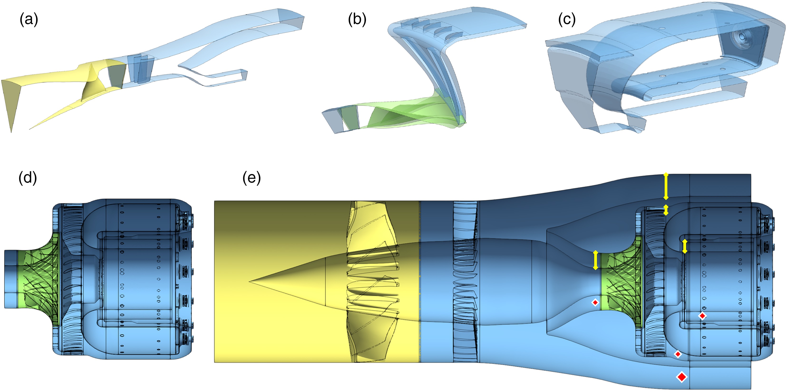
In this work, the operating point of study corresponds to take-off with opposite rotational speeds of 13,053 and 51,930 rpm for the fan and radial compressor, respectively. The total designed mass-flow rate is 13.846 kg/s with a by-pass ratio of 6.84. On the real engine, an effective suction of 1% of air is present within the compressor stage through a series of different outlets. In the present simulations this suction is mimicked at a position located on the compressor hub between the impeller and the radial diffuser. In order to ease the comparison against the design operating point, only the effective mass-flow rate after suction will therefore be considered (i.e. the mass-flow entering the combustion chamber). Last, the compressor works at a pressure ratio of 4.6 and the combustion chamber reaches temperatures of roughly 2,500 K and operates with a fuel to air mass-flow ratio of 0.018.

Numerical setup

The reactive as well as the non-reactive LES are performed with the code AVBP, the explicit unstructured and massively parallel compressible flow solver developed by CERFACS (Schönfeld and Rudgyard, 1999). All numerical predictions have been carried out using the explicit second-order scheme Lax-Wendroff (Lax and Wendroff, 1964) and the subgrid-scale model relies on the Wall-Adapting Local Eddy (WALE) viscosity model (Nicoud and Ducros, 1999). Note also that to reduce the computational cost of all simulations, a standard log-law is applied on all solid boundaries with slip conditions (Schmitt et al., 2007). This reduces the cost not only because the total number of cells is reduced but also because it increases the cell size at the wall and thus, the minimum time-step computed through a global Courant-Friedrich-Levy number is increased compared to a wall-resolved simulation. For combustion, the thickened-flame model (Colin et al., 2000) is used to account for combustion–turbulence interaction along with a reduced chemistry with 6 species and 2 reactions (Franzelli et al., 2010) where a purely gaseous premixed mixture is injected. In addition, the thickened-hole model (Bizzari et al., 2018) is introduced to represent the micro-perforations in the flame-tube. Non-reflective Navier-Stokes characteristic boundary conditions are used at inlet (Poinsot and Lele, 1992; Odier et al., 2019) and outlet (Granet et al., 2010; Koupper et al., 2015) without any kind of synthetic turbulence. This setup was shown to provide the best trade-off between accuracy and computational cost (Gicquel et al., 2012).

The variables specified as input parameters at inlet and outlet boundaries of the stand-alone simulations are the following. For the FAN + OGV, mass-flow rate and static temperature are defined at the inlet and static pressure at the outlets (different for the primary and secondary flows). The same approach is used for the CC domain whereas for the CoHP, total pressure and temperature are set at the inlet and static pressure at the outlet. The integrated simulation uses the same boundaries as the inlet of the FAN + OGV and the outlet of its secondary flow, along with the outlet of the combustion chamber.

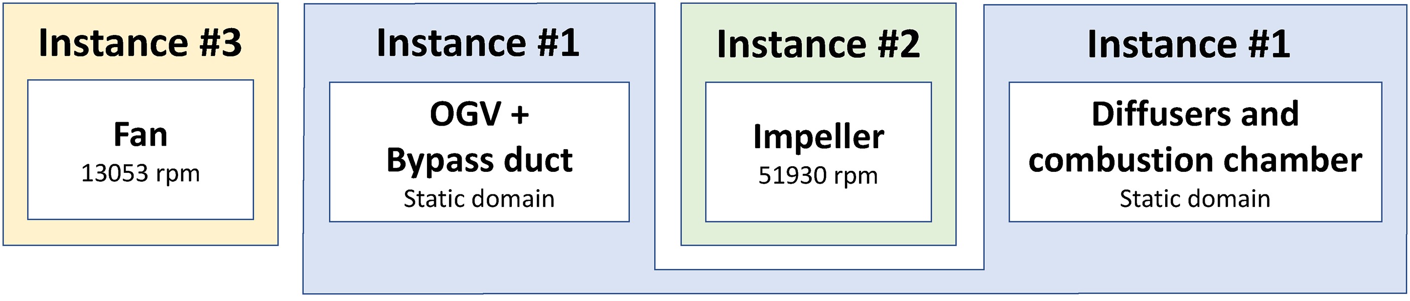
When it applies, the transfer of the flow between the static and rotating sub-domains is performed with an overset grid method over a common geometrical zone for the proper exchange of the necessary information (Wang et al., 2014; de Laborderie et al., 2018). AVBP is based on the SPMD paradigm for parallelism (Single Program - Multiple Data). In the case of this simulation separate in-code instances are automatically generated for static and rotating sub-domains. Each instance is coupled internally using the CWIPI library from ONERA (Refloch et al., 2011; Duchaine et al., 2015). Since there are two different rotational speeds, the integrated simulation FULLEST utilises three instances of AVBP to run as illustrated by Figure 2: one for the static sub-domain, one for the fan sub-domain, and one for the impeller sub-domain. The different instances for the stand-alone simulations are colour-coded according to Figure 1.

Figure 2.

Instance repartition according to the rotational speeds for FULLEST.

Details concerning the mesh used for each simulation are provided in Table 1 along with the wall-clock time per physical millisecond for the given number of cores. All meshes are unstructured and solely made of tetrahedral elements. The FAN + OGV mesh is similar to the “M1” mesh computed by Odier et al. (2017) with x+=y+=z+ of about 100 for a uniform refinement of 1 mm and a fan tip-gap discretisation of 17 cells. The CoHP mesh has a uniform mesh refinement of 0.25 mm, a wall refinement of 0.125 mm and between 7 to 9 cells in the tip-gap of the impeller following the recommendation by Dombard et al. (2018). This leads to average y+ values of about 150 on the hub and shroud and 75 on the walls of the blades and vanes. The CC mesh has a mesh size of 1 mm in the contouring casing and the outlet sections far from the walls. The swirler has a refinement of 0.2 to 0.4 mm, with the minimum at the walls and the dilution as well as primary holes are fully refined at 0.2 mm. The walls in the flame-tube are discretised at 0.25 mm whereas the interior coarsens from 0.4 to 1 mm as depicted in Figure 3a (Koupper et al., 2018). Overall, y+ of about 150 are obtained on the external walls, and about 50 on the walls of the flame-tube and swirler. The integrated domain FULLEST keeps the same level of discretisation as the stand-alone simulations at the walls. However the fluid mesh from the impeller to the exit of the combustion chamber has been coarsened by about 5% in the compressor and the combustion chamber to reduce the total number of cells. As a result, FULLEST which computes the full azimuthal 360 degrees of the machine, uses a mesh that is composed of 2,100 million cells which is over 1 order of magnitude higher than their stand-alone sectoral counterparts. In addition, the smallest cell in the whole domain is found in the tip-gap region of the impeller yielding the most limiting time-step for the entire simulation. Ultimately, the computational cost attains a value of about 300,000 core hours per physical millisecond, i.e. about 350,000 core hours per impeller revolution or about 1.4 million core hours per fan revolution. This integrated simulation has been performed through the access to the supercomputer Joliot-Curie (GENCI/TGCC) on 14,400 Skylake cores over several months consuming 31.6 million hours awarded by PRACE which is in agreement with the estimated cost and mesh size proposed by Anand et al. (2021) (second row in Table 1) for a full engine LES.

Figure 3.

Meridional cut of the mesh for the diffusers and the combustion chamber. (a) Target mesh (1 sector). (b) Coarse mesh (360°). (c) Adapted mesh (360°).

Initialisation and convergence of the stand-alone simulations

Performing the simulations of the stand-alone components has three goals. First, a data-base for each component without any interaction with its surrounding is obtained at a reduced cost. Secondly, such a prediction can then be used as a reference for the integrated simulation. Thirdly, as proposed by Pérez Arroyo et al. (2020), the final (i.e. converged at the correct operating point) instantaneous flow snapshot is used as initial solution of each specific component to launch the integrated simulation. The simulations FAN + OGV were initialised from previous LES solutions provided by Odier et al. (2018), updating the rotational speed of the fan and inlet as well as the outlet boundary conditions. In that case, note that a short trial and error setting period to find a satisfactory static pressure at the outlet boundaries was necessary to ensure the correct bypass ratio. Once the transient finished, data was acquired during 10 fan rotations for flow analysis. Note that as of today, one brute force possibility to initialise compressor simulations is to start with the flow at rest and then increase progressively the rotational speed and outlet pressure as explained by Dombard et al. (2018). Using this approach, convergence would be achieved within 10 revolutions. However in this work, the CoHP simulation was initialised directly from RANS solutions used to verify the geometrical modifications. Using this methodology, convergence was achieved within only 3 impeller revolutions saving up to 140,000 core hours with respect to the initialisation from a flow at rest. This CoHP simulation was then run until convergence and then for 10 rotations for analysis. The CC configuration was initialised from conditions at rest with first a mono-species non-reactive flow to converge the aerodynamics and design point at reduced cost. Once the solution is converged after approximately 20 ms, the gas air (represented by a single species in AVBP) is transformed into a mixture of N2, O2 and the species: CO, CO2 and H2O, which are set to zero. Then fuel is injected in a gaseous form inside the vaporiser for about 5 ms until a recirculation zone of mixed fuel and air is generated in the combustion chamber. The flow is then ignited by adding an energy deposition that mimics a spark. To finish, the simulation is converged after a transient period of about 25 ms with a flame properly positioned in the flame-tube. Data is then acquired for 50 additional milliseconds for flow analysis which corresponds to about 5 convective flow-through times which is enough to converge root-mean-square (RMS) values.

Generation of the integrated domain and associated mesh

The static sub-domain for FULLEST is composed of the OGVs, the bypass duct, the radial and axial diffusers as well as the combustion chamber as illustrated in Figure 1e. Furthermore, it is geometrically divided in aft and forward disconnected regions by the impeller sub-domain. The mesh and initial solution of the fan sub-domain, the forward region of the static sub-domain (from fan outlet to compressor inlet) and the impeller sub-domain can be easily constructed by azimuthal repetition of sectoral meshes using the in-house package for manipulating unstructured computational grids HIP (Müller, 1999). The tool HIP is able to merge all replicated surfaces creating a single mesh and associated solution file for all 360° sub-domains. In fact, only the mesh for the fan sub-domain from FAN + OGV is conserved intact. The sectoral meshes for the OGVs and bypass duct regions are first regenerated with the same refinement parameters as FAN + OGV, taking into account the right geometry connecting to the impeller. For the impeller sub-domain, a new sectoral mesh is created with new refinement parameters. Then, the mesh for the fan sub-domain and the one regenerated for the OGVs and bypass duct region can be repeated 13 times and rotated while the impeller can be duplicated 10 times.

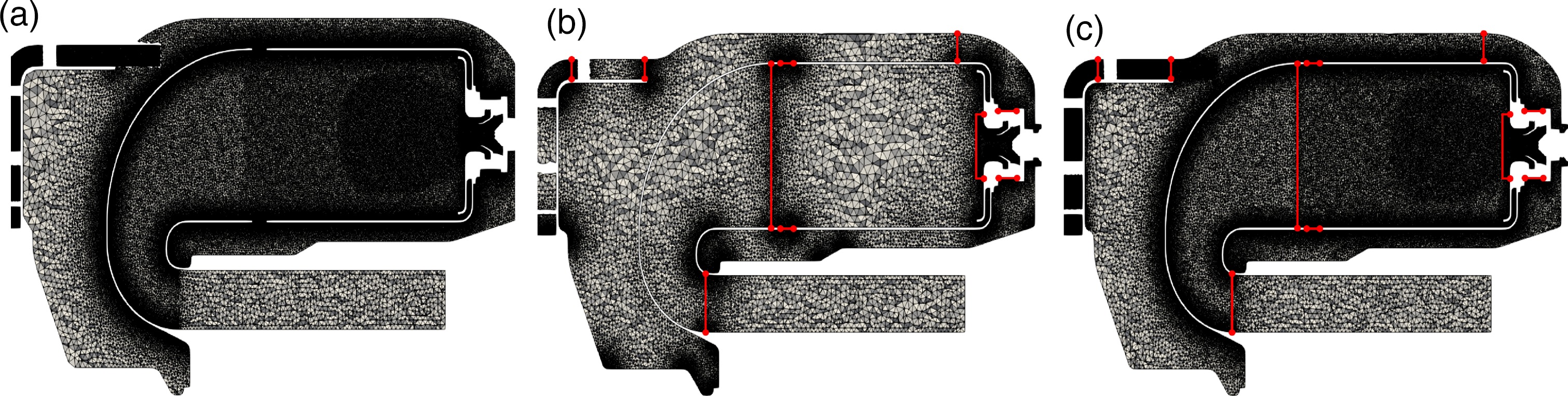
A particular challenge arises for the aft region of the static sub-domain, i.e. the diffusers and the combustion chamber because they differ in their azimuthal periodicities. For this specific static component junction, if the sectoral meshes were to be repeated azimuthally, a non-conformal interface (not supported by AVBP) would appear between the axial diffuser and the combustion chamber regions. Several solutions were considered to overcome this problem. The generation of a fully 360 degrees refined mesh including the diffusers and the combustion chamber was discarded due to memory limitations to generate such a heavy mesh on our visualisation machine with 64 GB of RAM. The addition of another AVBP instance for the combustion chamber was also tested on a sectoral configuration but it led to an increase in computational cost of over 20% due to the additional instance and its new interfaces. Ultimately, the solution retained for this work was to generate a 360 degrees coarse mesh that was then refined following a given metric using the library MMG (Dapogny et al., 2014; Daviller et al., 2017). To refine and adapt the mesh, a metric is constructed using the meshes from the stand-alone sectoral simulations as the target mesh (Figure 3a), and using the 360 degrees coarse mesh as input (Figure 3b). The metric is then applied to the local edge size of the cells and it is computed by dividing the cell-averaged edge size of the coarse mesh by the target edge size of the sectoral simulation at each node of the coarse mesh. The edge size value of the target mesh is interpolated on the coarse mesh in order to be able to perform this operation. The mesh adaptation was performed only on the aft region of the considered sub-domain (static sub-domain of CoHP + CC) and due to other technical limitations (currently, MMG is only capable of handling 32-bit integers limiting the size of the domain it can handle), the sub-domain was further divided in 8 zones as depicted in Figure 3b by the red boundaries. Each zone is therefore adapted independently and then merged together with HIP. In order to do so and avoid non-matching interfaces, the boundaries of each zone are generated to the target sizes of the initial coarse mesh and are not modified during the adaptation process. Finally, the full static sub-domain for FULLEST is obtained by adding together both aft and forward regions. A view of the resulting mesh for the combustion chamber is illustrated in Figure 3c. Although cumbersome, this procedure was the only way to generate this extreme mesh.

Setup of the initial solution for the integrated domain

As mentioned above, the initial solution file for the forward region of the engine (including the impeller) was generated by an azimuthal duplication of the last instantaneous converged results from the corresponding stand-alone simulations. Prior to this duplication, the number of species is again transformed following the same procedure as the one used in the stand-alone CC, i.e. change from the mono-species air to the mixture of species used to model combustion and then interpolated in the intermediate sectoral meshes mentioned above for the fan, OGVs and impeller. This is also performed in the axial and radial diffusers. The solution for the aft region (diffusers and combustion chamber) is then obtained in a similar manner as Pérez Arroyo et al. (2020) by performing two partial piecewise linear gradient-based interpolations. First, the CC solution is azimuthally repeated and partially interpolated into the 360 degrees refined CoHP + CC mesh. Then, in the second step, the azimuthally repeated solution from the diffusers is partially interpolated onto the CoHP + CC mesh, where the previously interpolated solution is also read and overwritten in the axial diffuser as well as part of the contouring casing.

Efficient mesh partitioning for the integrated domain

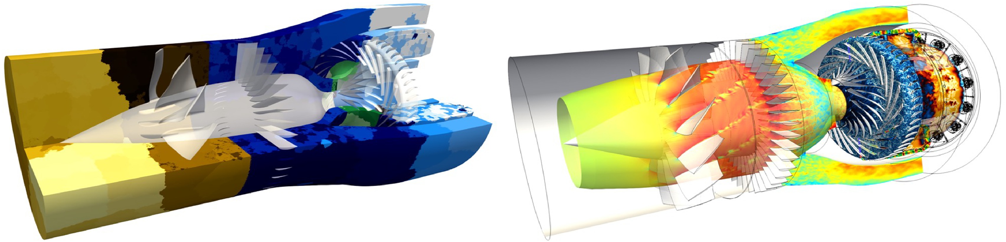
Finally, the mesh and associated solution need to be partitioned in order to launch the simulation in parallel. This was performed for FULLEST utilizing the hierarchical domain decomposition and load balancing tool TREEPART (Mohanamuraly and Staffelbach, 2020). Indeed, FULLEST is out of scope of standard domain decomposition techniques due to the large number of elements and the large number of cores used in the simulations. Traditional domain decomposition libraries such as Parmetis (Karypis and Kumar, 1998) or Pt-Scotch (Chevalier and Pellegrini, 2008), often fail with core counts over 4,000 and with meshes over 700 M elements in the author's experience. This is due to the important memory requirements and global communications used in these libraries. TREEPART was built to account for the local computing machine topology at the hardware level and minimise global communications. In fact it uses one-side MPI 3 communications for all exchanges and only relies on Parmetis for low level graph decompositions. TREEPART can be used at runtime within the code or off-line to generate a parallel mapping file called el2part (each element of the mesh is mapped to a given number of partitions) than can be read by AVBP to perform the simulation reducing initialisation times and ensuring reproducibility. An illustration of the final partitioning is shown in Figure 4 (left).

Figure 4.

Three-dimensional illustrations of FULLEST. (left) Illustration of the partitioning over 8,820 cores for the static domain (in blue colours), 2,880 cores for the compressor instance (in green colours) and 2,688 cores for the fan instance (in yellow colours). (right) Instantanous contours of FULLEST depicting Mach number in the forward region, density gradients in the compressor, pressure fluctuations in the contouring casing and temperature in the combustion chamber.

From sectoral and stand-alone to 360 degrees and integrated simulations

The simulation is initialised on the CoHP + CC domain for 6 impeller revolutions in order to ensure that the flow is correctly established between the compressor stage and the combustion chamber at a reduced cost. After this time, the remaining forward section of the engine is added (FULLEST case) and the simulation is run for 26 additional impeller revolutions to eliminate the transient related to the integration from the whole domain and acquire data for analysis. The complexity of this simulation is demonstrated in Figure 4 (right) with an instantaneous snapshot of the entire domain. Figure 5 illustrates the convergence of integral values at 4 axial locations in the domain (see Figure 1e): at the outlet of the secondary flow, at the inlet of the compressor, at the exit of the axial diffuser and at the exit of the combustion chamber. Results are normalised with the zero-dimensional values at those sections. These are averaged quantities in time (steady values) and space (e.g. over an axial plane at the inlet of the machine). These values are used to define the main characteristics of the engine in a design process. The outlet of the secondary flow (Figure 5a) features a transient in mass-flow rate m˙ which converges after 2.5 fan revolutions and total pressure P_t as well as total temperature T_t stabilise after 1.5 fan revolutions. At the impeller inlet (Figure 5b), m˙ undergoes a deficit at the end of the first impeller revolution but it stabilises back after 3 revolutions. The apparently temporary loss of mass-flow in the domain is possibly due to a combination of interpolation errors and the adaptation to the new boundary conditions at the inlet of the impeller. When the fan and OGV domains are added, all three variables are suddenly reduced but they stabilise and recover within 6 impeller revolutions. The variance of each variable has been increased with respect to the values at the end of the CoHP + CC simulation which already shows an impact of the unsteadiness introduced by the presence of the Fan and the wakes generated by the OGV. Results after the axial diffuser shown in Figure 5c barely change. Only a minor variation is observed which lasts about 1 impeller revolution after each integration. At the exit of the combustion chamber (Figure 5d), due to its large characteristic time, it is not possible to confirm an effect of the integration on the integral values.

Figure 5.

Convergence plots of normalised integral values for (solid black) m˙, (dash-dotted red) Tt and (dashed blue) Pt at four different cross-sectional positions noted in yellow in Figure 1e. Values are normalised by the ones from the thermodynamic cycle. (a) Secondary flow outlet. (b) Impeller inlet. (c) Axial diffuser trailing edge. (d) Combustion chamber exit.

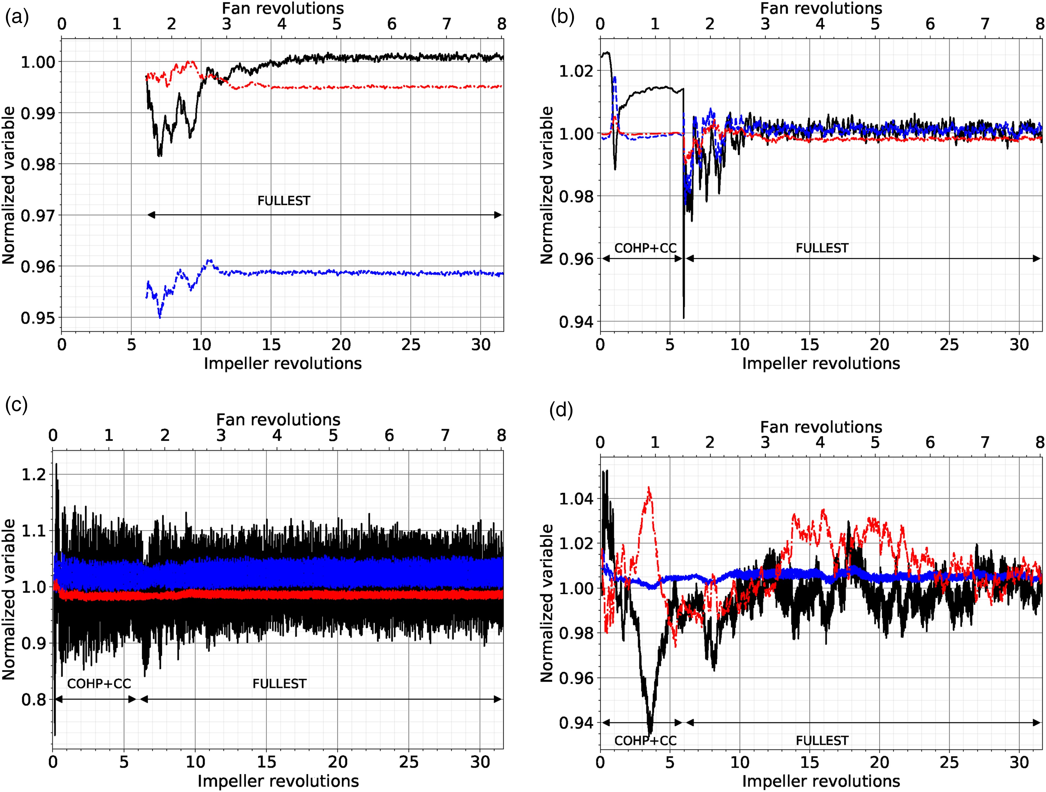
Table 2 shows the comparison against the design operating point for both stand-alone and integrated simulations computed over the last 10 impeller revolutions at different positions of the engine for m˙, total temperature Tt and total pressure Pt deviations expressed in percentage. The subtraction between given values provides a first approximation of how much the simulation can be impacted by the integration. The mass-flow rate is correctly recovered with differences of less than 1% between the simulations and the operating point and between the stand-alone and the integrated simulations at all locations listed in Table 2. Deviations above |±1%| (highlighted in bold) found for Tt and Pt at some positions are discussed in the following. At the fan inlet, a relative error of −1.42% and −0.74% are reached for Pt. This difference, although not substantial could be linked to the fact that the inlet is modelled with a straight duct instead of considering the full nacelle. As previously explained, the static pressure was modified for the secondary flow outlet to obtain the right bypass ratio. In addition, as before, the geometry outside the nacelle is not taken into account in the simulation. As a consequence, a relative error greater than 4% for Pt is achieved for all computations. At the inlet of the combustion chamber, values differ depending on the simulation. For the CoHP case, Tt presents a difference of −2.02% whereas a discrepancy of 1.85% is found for Pt in the CC case. Differently, as static temperature (CC) and static pressure (CoHP) are set at the inlet and outlet boundary conditions, respectively, these values are closer to the operating point. Similarly, because the FULLEST case does not have any boundary condition at the inlet of the combustion chamber, both variables slightly differ from the thermodynamic cycle. Despite the disparity in Pt, when this one is measured on the primary and dilution holes (only values at the exterior primary hole are shown in Table 2 for simplicity) and compared against the designed operating Pt at the inlet of the combustion chamber, a similar Pt is obtained for both simulations. This suggests that even though Pt differs from the operating point at the inlet of the combustion chamber, the values seen by the flame-tube should be in agreement with the operating point. Last, values at the outlet of the combustion chamber show similar Tt for both simulations.

During the initialisation, the flow does not only experience the transient developed from adding other components but also an azimuthal decorrelation. This occurs because the initial solution has been azimuthally repeated from the sectoral simulations. This decorrelation is illustrated in Figure 6 using temporal signals extracted from nodes at similar axial locations as the ones used for Figure 5. The decorrelation is calculated by computing the evolution of the Pearson correlation coefficient,

Figure 6.

Azimuthal decorrelation plots of local signals for (black) ux, (red) T and (blue) P at different positions noted in red in Figure 1e. Solid lines represent the decorrelation with the adjacent azimuthal sector whereas dashed lines illustrate the decorrelation with the opposite azimuthal sector. (a) Secondary flow outlet. (b) Impeller inlet. (c) Exit of the axial diffuser. (d) Combustion chamber exit.

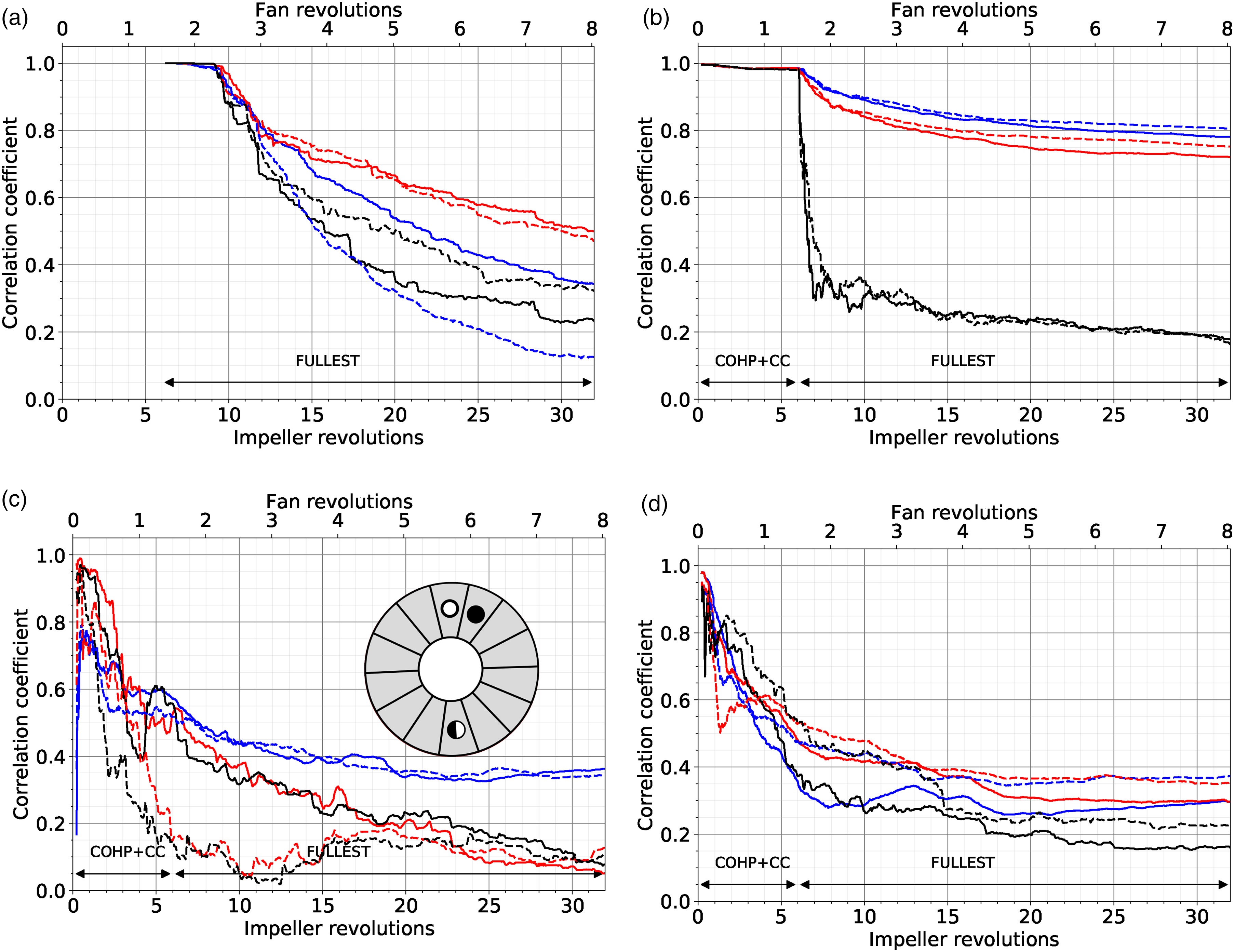
where n goes from 1 to the total number of iterations N computed in the simulation. The signal X{x1,…,xn} is fixed and used as reference whereas signal Y{y1,…,yn} is extracted from the adjacent azimuthal sector or the opposite azimuthal sector with respect to the position of signal X. The evolution of the correlation coefficient is shown for the axial velocity (ux), P and T at a position close to the outlet of the secondary flow in Figure 6a. All variables remain unaffected for the first fan rotation and then start to drop at different rates. Temperature correlations from both axial positions in the machine drop at the same rate whereas different behaviours are obtained for ux and P. Correlations of ux are higher on the closest signal as it would be expected whereas this occurs for the farthest signal for the pressure correlations. Nonetheless, this could be explained by the presence of azimuthal modes synchronised at these locations. At the inlet of the impeller (Figure 6b), the solution remains azimuthally periodic until the forward section of the static domain is added (case FULLEST). Then, as the periodicity of this section differs from the one of the compressor and receives the wakes from the fan and OGVs, the correlation coefficient suddenly drops for ux and stabilises about 2 fan revolutions later. Pressure and temperature on the other hand decay at a slower rate and to higher values than ux. A different behaviour is found after the axial diffusers and at the exit of the combustion chamber as depicted in Figure 6c and 6d. As a result of higher turbulence levels coming from each component, the flow decorrelates much faster at these positions than the previous ones. This occurs from the start of the first integration (CoHP + CC). The second integration (case FULLEST), has no visible impact on the correlation coefficient and they stabilise after about 15 impeller revolutions for the three variables. Results for FULLEST are thus considered azimuthally decorrelated and will not have any history effect coming from the stand-alone simulations.

Upstream propagating shock-wave from the compressor

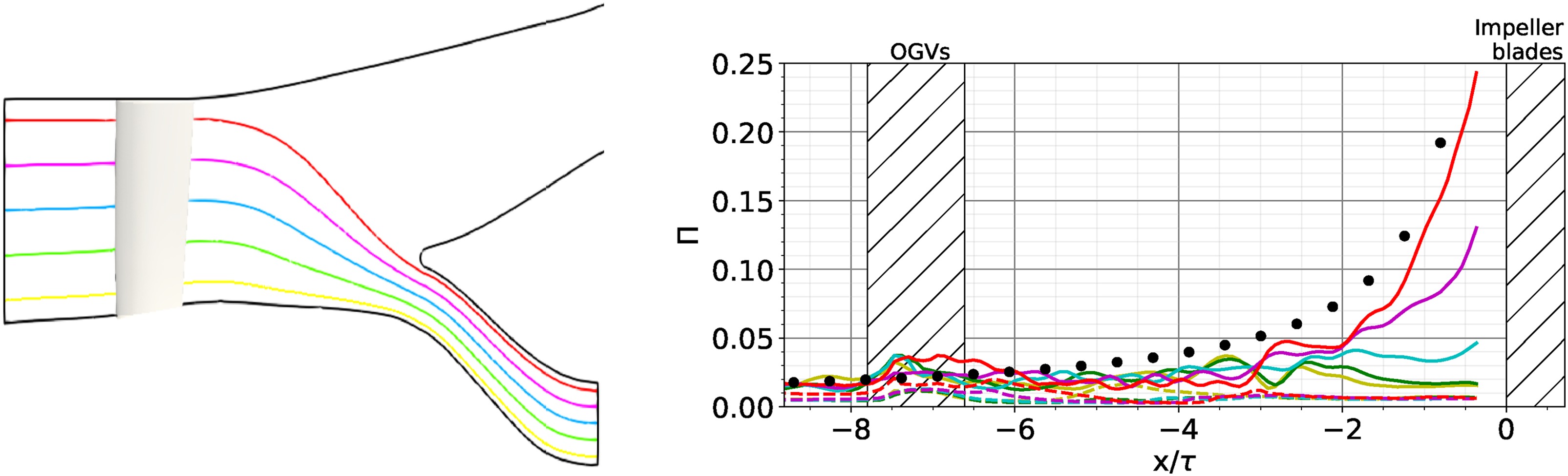
The flow topology generated at the inlet of the impeller is presented since it has an impact on the flow around the fan and OGVs. At take-off conditions, the compressor operates in transonic conditions in the rotating frame of reference of the impeller and a shock-wave is formed at the leading edge of the impeller which propagates upstream towards the fan. The shock is generated due to the high impeller rotational speed needed to attain the designed pressure ratio at take-off (Ferri, 1964). The flow field is therefore dominated by a strong shock as depicted in Figure 7 using an instantaneous field at 70% of the normalised hub-to-shroud distance (denoted hereafter h/H). Although the Mach number remains below 0.8, the relative Mach number (i.e. the Mach number in the rotating frame of reference) attains values of up to 1.4. This translates in a pressure jump of about 30 kPa across the shock.

Figure 7.

Illustration of the upstream propagating shock at 70% h/H generated at the leading-edge of the impeller. Black iso-line refers to the sonic line in the relative frame of reference.

Since the shock is anchored at the leading edge of the impeller, it rotates with it. This discontinuity is seen as a propagation in the absolute frame. Disturbances that propagate at subsonic conditions are known to decay exponentially with distance, however, because shock wave evolution is principally an inviscid phenomenon as demonstrated by Prasad (2003), it decays as the inverse of the axial distance from the leading edge (Morfey and Fisher, 1970; Hawkings, 1971). Indeed, far from the rotor and for high pressure jump ratios noted Π, the shock wave can be expressed for two-dimensional flows as,

where γ is the specific heat ratio, Mx and Mrel are the axial and relative Mach number, respectively, τ is the distance between blades and Π is the ratio between the pressure difference and the mean pressure across the shock. The pressure jump Π is approximated here by the ratio between twice the root-mean-square and the average static pressure averaged azimuthally so that it can be compared against the FAN + OGV case. The shock decay is illustrated in Figure 8 for several h/H ratios from the impeller to the OGVs through the h/H iso-lines depicted in Figure 8. Since this shock is mainly generated on the upper half of the blade span, i.e. above 50% h/H, the increase in Π with h/H dominates this upper section as shown in Figure 8. Despite all the approximations, the analytical expression (Equation 2) applied using values at 90% h/H, correctly captures the decay of the shock and shows its ability to propagate upstream through the machine. As expected, FAN + OGV results do not show the high pressure jump of the shock since there is no impeller in the simulation. Further details about this first direct effect of the integration of the fan and OGVs with the compressor is elucidated in the companion paper (Pérez Arroyo et al., 2021).

Figure 8.

Normalised pressure jump Π at different values of h/H: (yellow) 10%, (green) 30%, (cyan) 50%, (violet) 70%, (red) 90%. (solid) FULLEST, (dashed) FAN + OGV. (∙) analytical expression (Equation 2).

Symbols

Acronyms