
Introduction
Increasing reliability and efficiency of gas-turbine engines, while reducing pollutant and noise emissions is one of the main goals of industry. Currently, engines are designed by several departments that focus on different engine components (compressor, combustion chamber, turbine and others). While the individual components may behave within design margins, the assembled engine could exhibit overall poorer performance due to integration effects, i.e. interactions between components that were unknown or not considered in the design phase of each individual component. Here, the integration effects are investigated with a massive 2,100 million cells 360 azimuthal degrees reactive Large-Eddy Simulation (LES) of a turbo-fan engine composed of the fan, compressor and combustion chamber. Performing a single LES, although costlier, simplifies the transfer of unsteady phenomena such as turbulence and pressure fluctuations between components since there are no boundaries to define at interfaces.
This work is the continuation of the companion paper (Pérez Arroyo et al., 2021) where the methodology and initialisation to perform such a simulation are explained in detail and are briefly recalled in the following. In order to reduce the convergence time (computational cost), the initial solution of the integrated simulation (referred hereafter as FULLEST) is constructed from stand-alone sectoral LES of the fan, compressor and combustion chamber. This generates as well a three-dimensional data-base of each component used for comparison. The generation of the unstructured mesh of over 2,100 million cells for FULLEST consists of two operations to yield the best trade-off to solve potential machine dependent memory limitations. The domains of the stand-alone simulations that are geometrically isolated such as de fan, the static sub-domain of the outlet-guide vanes (OGVs) and the impeller are repeated azimuthally using the in-house package for manipulating unstructured computational grids HIP (Müller, 1999). The second procedure is applied to the diffusers and the combustion chamber that do not share the azimuthal periodicity. In this case, a coarse mesh is generated first for the full azimuthal extent (360 degrees) from the exit of the impeller to the exit of the combustion chamber. Then, the mesh is refined using the library MMG (Dapogny et al., 2014; Daviller et al., 2017) where a metric is constructed using the meshes from the stand-alone sectoral simulations as the target mesh. FULLEST computation converges to an operating point with less than 0.5% difference in in mass-flow, total temperature and total pressure compared to the stand-alone simulations with an overall 1% error if compared to the designed thermodynamic cycle. Last, the flow topology of the impeller is introduced. At take-off conditions, the compressor works at transonic conditions and generates a shock anchored at the leading edge of the impeller. Since, it rotates with it, this discontinuity is seen as a propagation in the absolute frame.
The impact of this shock on the fan stage is studied in more details in this work which is structured as follows. First, the configuration is briefly introduced. Then results of the integrated simulation are analysed and compared against the stand-alone LES predictions of each component for the fan, compressor and the combustion chamber. Finally, main conclusions are listed.
Configuration
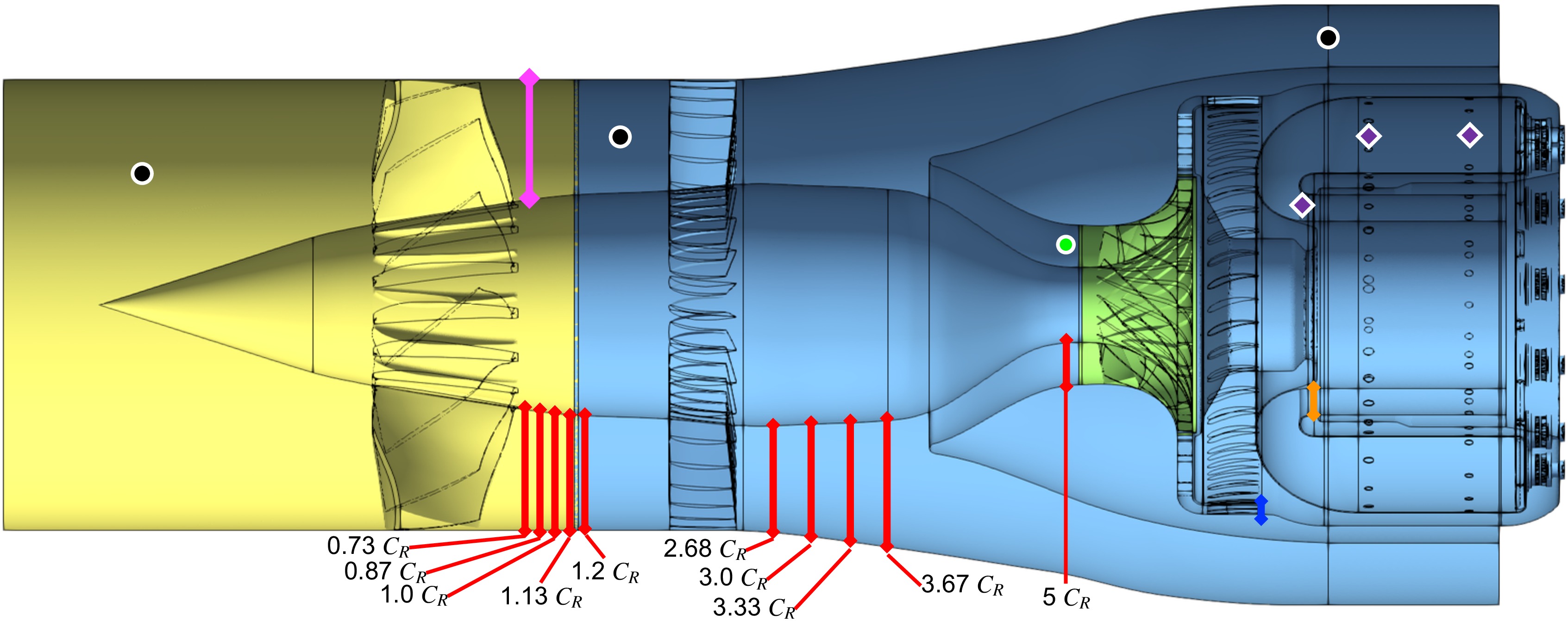
The DGEN-380 demonstrator engine is studied here numerically at take-off conditions in a single reactive wall-modelled LES performed with the explicit unstructured and massively parallel compressible flow solver AVBP developed by CERFACS (Schönfeld and Rudgyard, 1999). The domain contains the full 360 azimuthal degrees LES of: the fan rotating at 13,053 rpm with 14 blades; 42 outlet-guide vanes; the radial compressor composed of 11 main blades and 11 splitter blades rotating at 51,390 rpm (in the opposite direction of the fan), as well as a radial and an axial diffusers composed of 22 and 55 vanes, respectively; and the annular combustion chamber with primary and dilution holes as well as 13 double contra-rotating swirlers. Results are compared against stand-alone simulations of each component that are performed on an azimuthal sector of 360/14 degrees for the fan and OGVs (noted as FAN + OGV), 360/11 degrees for the compressor including the radial and axial diffusers (noted as CoHP) and 360/13 degrees for the combustion chamber (noted as CC). The integrated domain FULLEST shown in Figure 1 is constructed by azimuthal repetition of the sectoral domains to have a fair comparison between simulations. Nonetheless, besides their azimuthal extent, the domains still present some differences which are listed in the following. The outlet of the primary duct in FAN + OGV and outlet in CoHP are extended axially to ease the evacuation of turbulence. Similarly, the inlet of CoHP and CC are also axially extended. The diffuser vanes were not considered in CC because its azimuthal periodicity is different than the one for the chamber. More details about the domains, operating point, numerics and mesh specifications can be found in the companion paper (Pérez Arroyo et al., 2021).
Figure 1.
View of the 360° FULLEST domain. Blue depicts the static sub-domains, and green and yellow the rotating sub-domains depending on its rotational speed. Lines and markers in Figure 1 are used as a reference throughout this work.
Results
In this section, results from FULLEST are compared against the stand-alone simulations to analyse the impact of the integration on the aerodynamics and acoustics. Time-averaged fields and spectra are presented for all the components starting with the fan, following with the compressor and finalising with the combustion chamber. Three-dimensional information (e.g. axial, meridional or radial cuts) extracted from the integrated simulation are azimuthally averaged onto a single sector (which angles depend on the component of study) in order to increase its statistical convergence. This is performed by splitting the solution for all azimuthal sectors and interpolating it on the mesh of one sector which angles coincide with the stand-alone sectoral simulation. Other results such as the Power Spectral Density (PSD) of local temporal signals are also azimuthally averaged using one signal per sector which has a similar effect as the classical windowing performed in signal analysis.
Comparison of the fan and bypass duct predictions
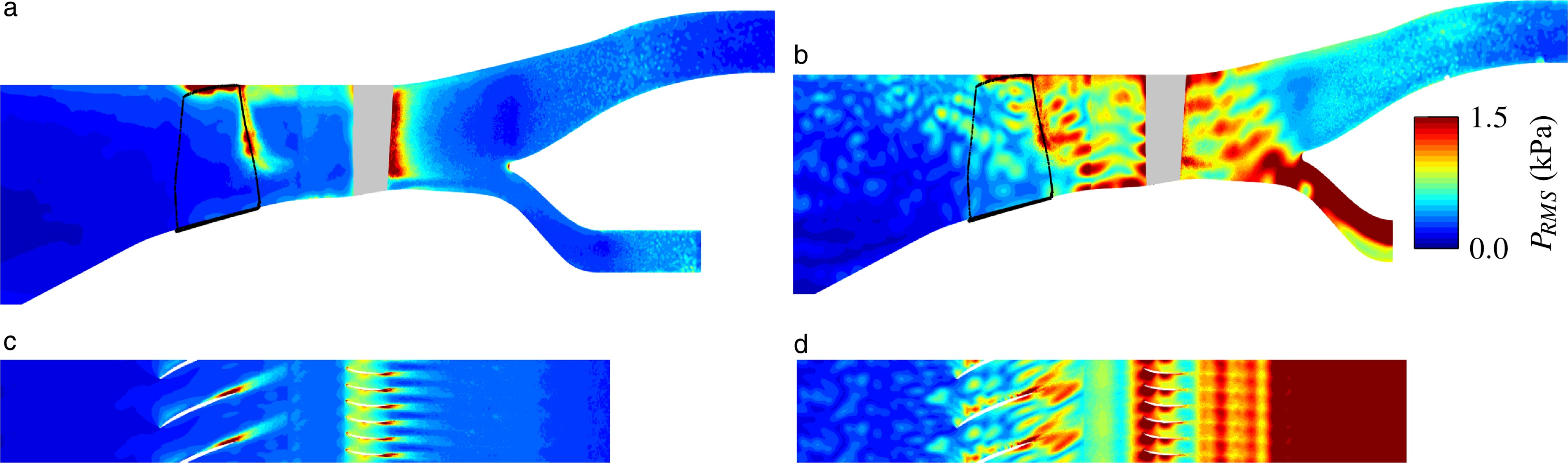
As stated in Pérez Arroyo et al. (2021), at take-off conditions, the pressure fluctuations in the bypass duct and the fan are dominated by the shock generated at the transonic impeller. This effect is clearly visible on the static pressure root-mean-square
Figure 2.
P RMS h / H h / H
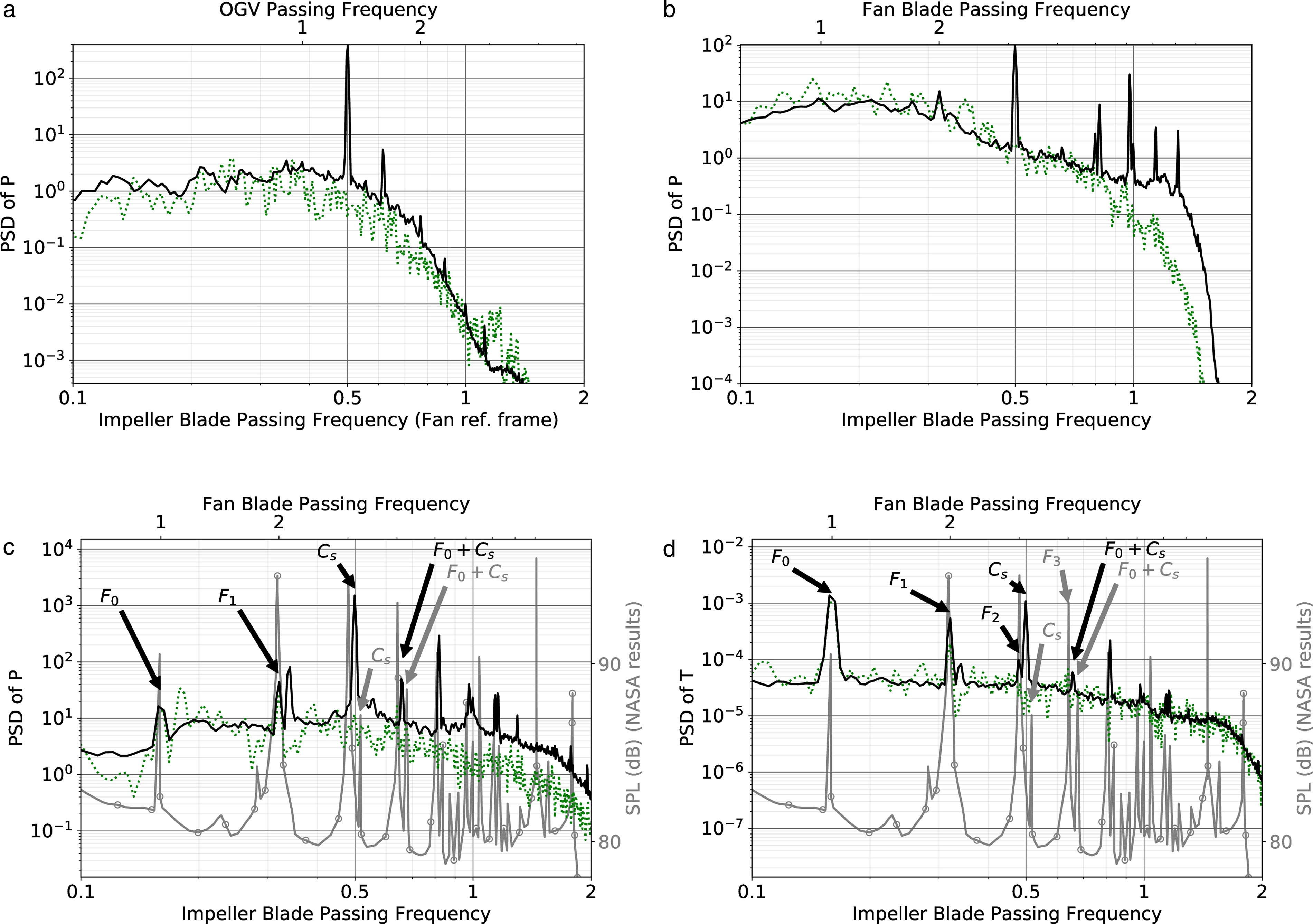
Indeed, a tone emerges at half the relative impeller Blade-Passing Frequency (BPF) as illustrated in Figure 3a when the pressure spectra is analysed on numerical probes located before the fan. Here the impeller BPF is considered as relative because the probe is located on the rotating sub-domain of the fan and it rotates with this domain. The relative impeller BPF is computed by adding both rotating speeds of the fan and the impeller (or subtracting them if they were turning in the same direction) before multiplying by the number of blades. In this work, the impeller BPF is computed with all 22 blades of the impeller and thus, the shock which is generated at the trailing edge of the 11 main blades is perceived at half this BPF (relative or not). This peak in the spectrum, hereafter referred to as
Figure 3.
Power spectral density (PSD) at different locations noted in black in Figure 1. (solid black) FULLEST, (dotted green) FAN + OGV, (solid gray) NASA SPL. (a) Inlet of the fan. (b) Secondary flow duct. (c) Position between the fan and the OGVs. (d) Position between the fan and the OGVs.
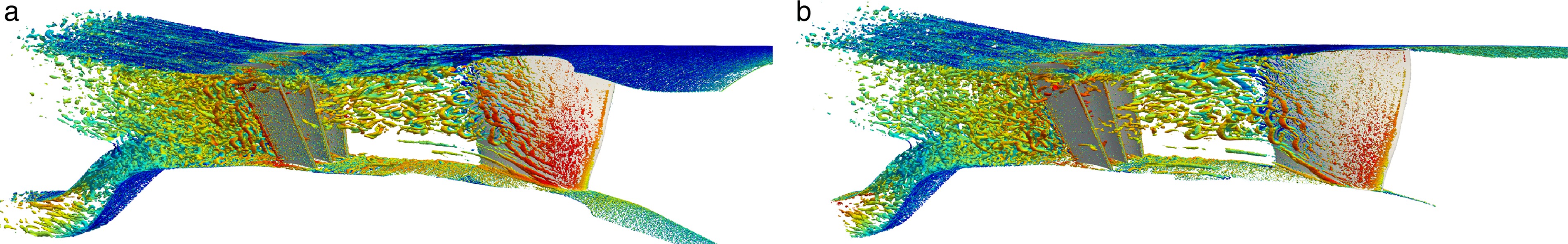
As a first attempt to unravel the possible impact of such intense pressure fluctuations on the flow topology, instantaneous contours of Q-criterion coloured by
Figure 4.
Instantaneous Q-criterion contours coloured by u x
In order to further study the impact of
Figure 5.
PSD and Contours at the axial position noted in magenta in Figure 1. (a) FAN + OGV. (b) FULLEST. (c) FAN + OGV. (d) FULLEST. (e) FULLEST (DFT). (f) Integral of DFT at all frequencies. (black)u x P
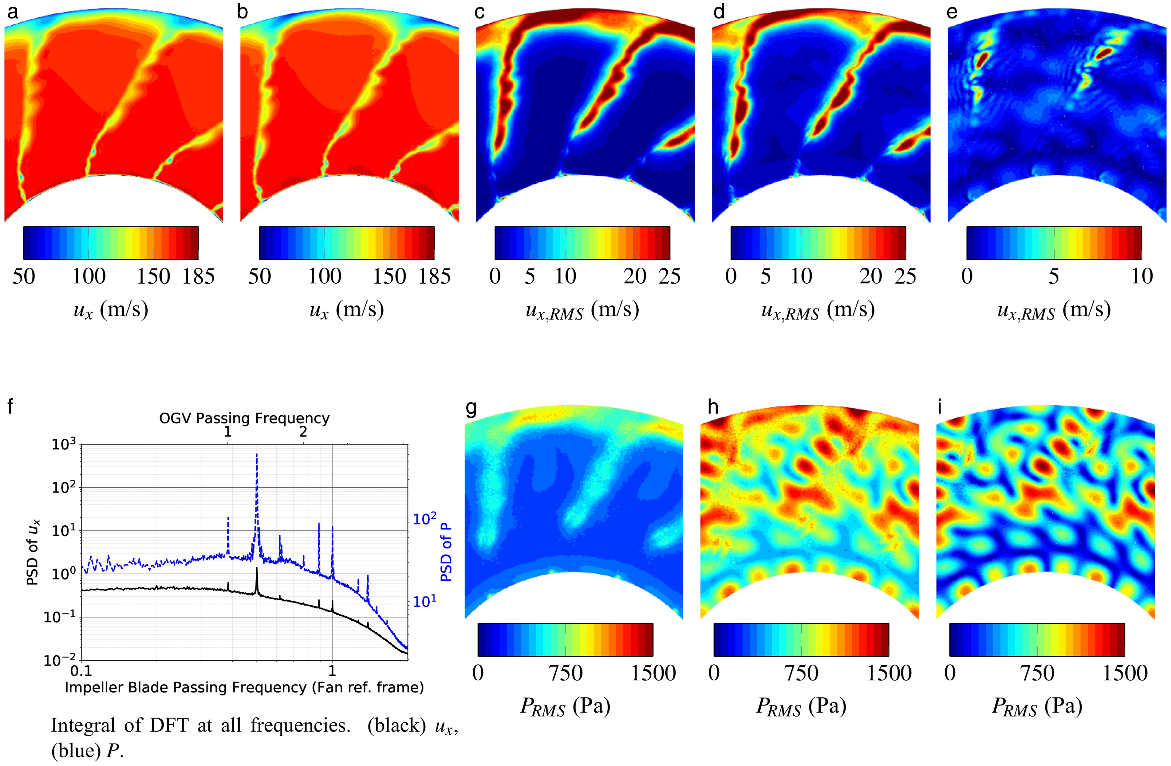
The impact of
Figure 6.
Azimuthal profiles of u x u x , RMS h / H u x , mean θ s = 360 / 14 ∘ C R h / H
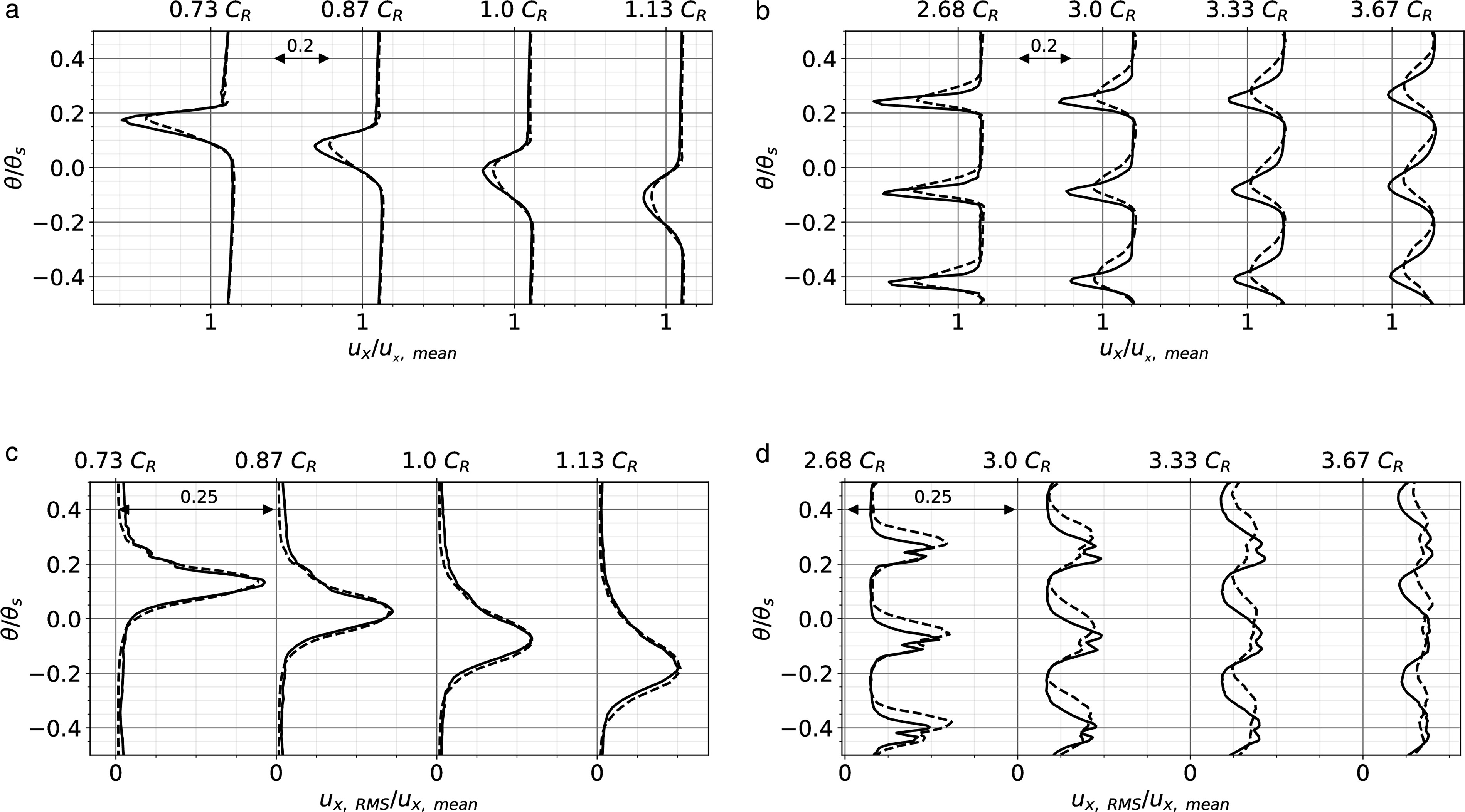
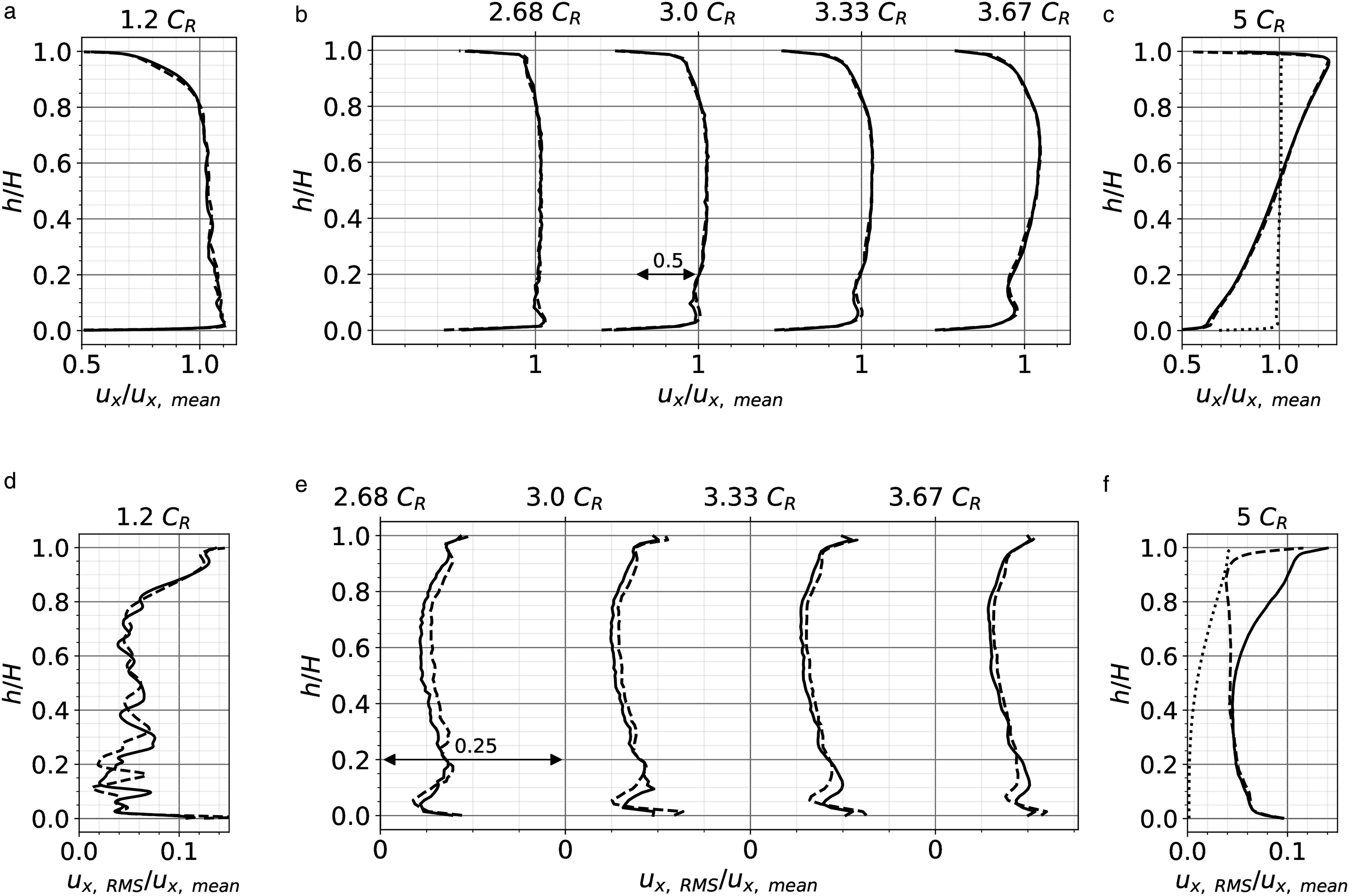
Last, the azimuthally averaged radial profiles are analysed on the static sub-domain and shown in Figure 7. The time-averaged wake of the fan (Figure 7a) presents similar results for both simulations which demonstrates that even if the wakes have slightly different velocity deficits, their azimuthally averaged value remains the same. This also applies to the development of the TLV near the shroud which is not impacted by
Figure 7.
Radial profiles of u x u x , RMS ( u x , mean ) C R h / H
Comparison of the compressor and diffusers predictions
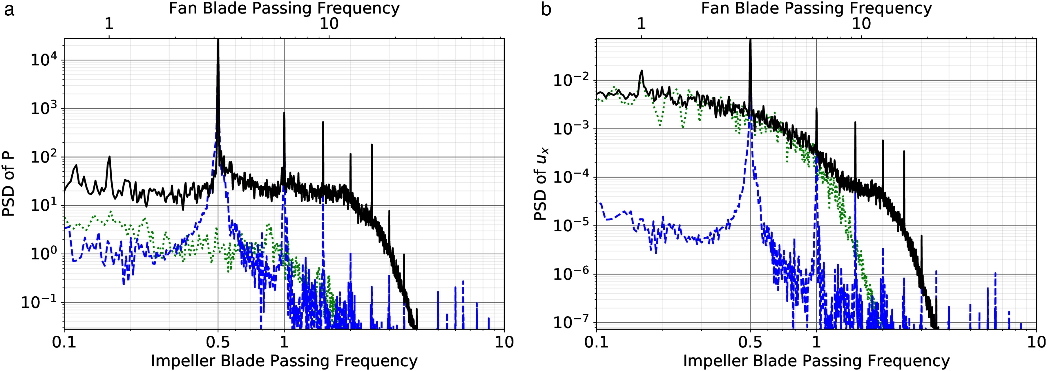
The interaction from the upstream propagating shock, the fan and OGVs results in an increase
Figure 8.
Power spectral density (PSD) at the inlet of the impeller in the static domain as depicted in Figure 1 in green. (solid black) FULLEST, (dotted green) FAN + OGV, (dashed blue) CoHP.
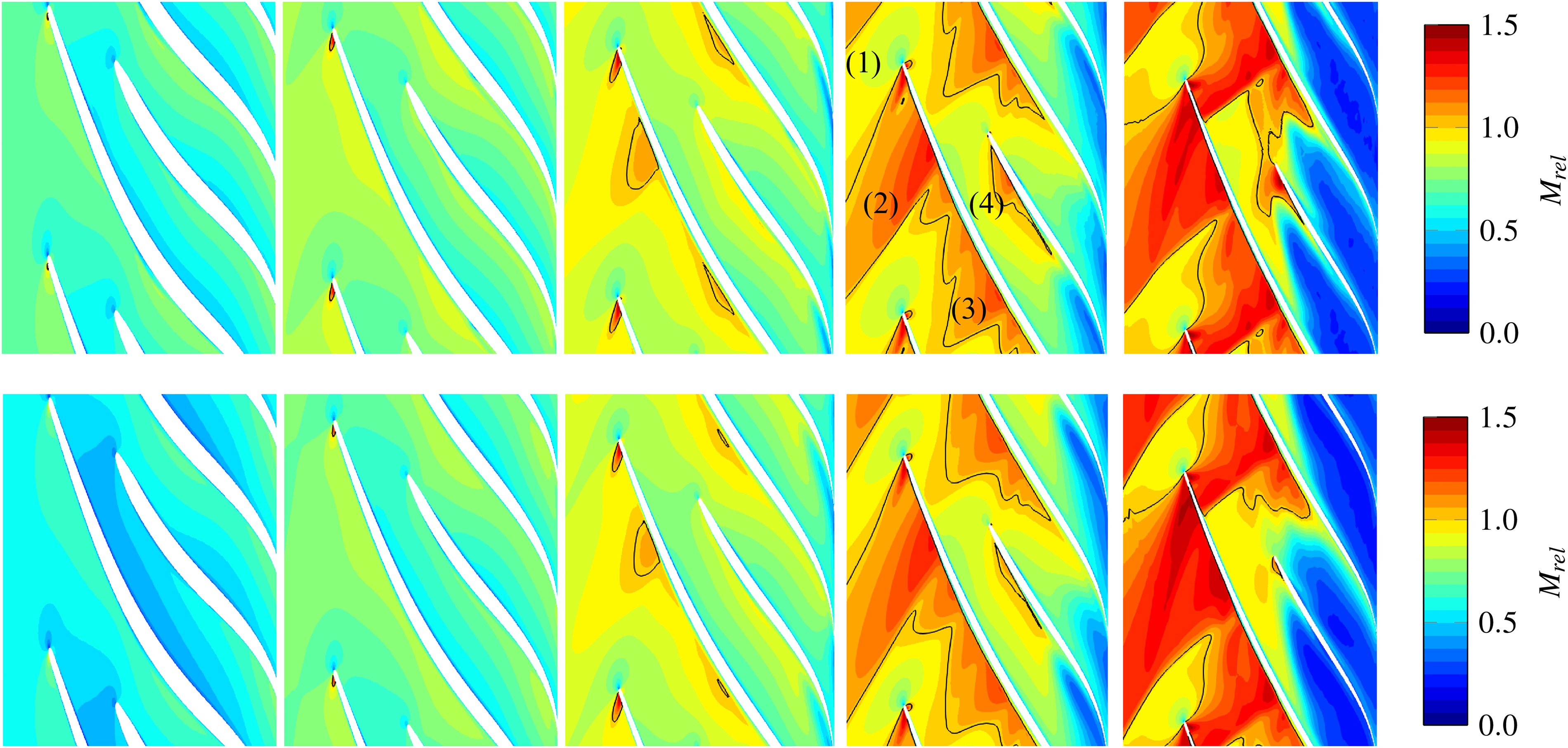
The flow topology is now compared between CoHP and FULLEST. Particular attention is drawn to the topology at the inlet of the impeller and at the interface between the impeller and the radial diffuser. The relative Mach number contours (computed on the relative frame of reference of the impeller) are shown in Figure 9 at different heights of the channel. Overall, results are similar between both simulations. Nevertheless, some specific differences can be identified and these are described in the following for the sake of rigour. At this location, four regions highlighted in Figure 9 can be distinguished. At the leading edge of the main blade the flow accelerates on the suction side and presents a sonic region all along the blade span for FULLEST. In CoHP, this sonic region is less intense and it does not appear at 10%
Figure 9.
Relative Mach number contours at different h / H h / H
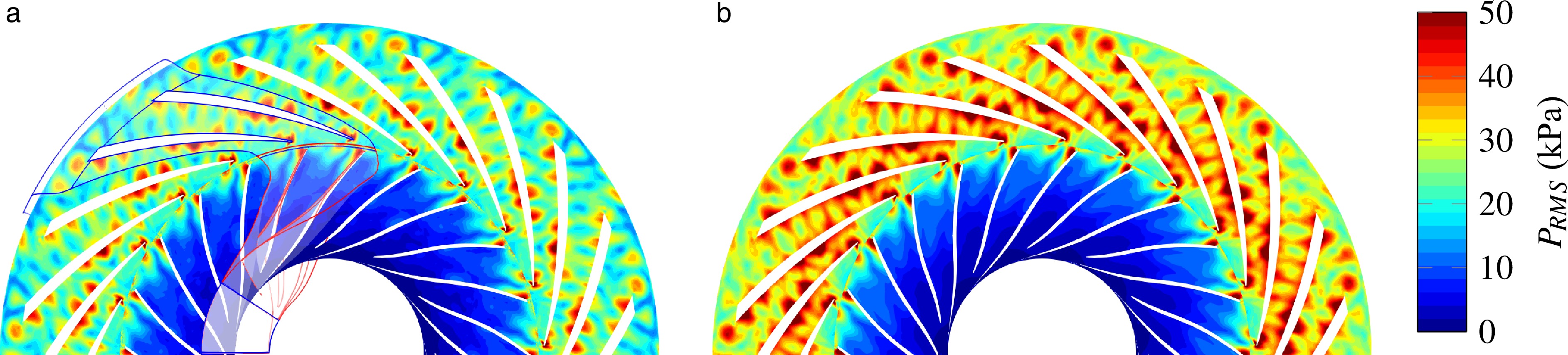
The waves that propagate through the radial diffuser leave a characteristic pattern in the static pressure RMS for both simulations as depicted in Figure 10 which reaches values up to 50 kPa near the vanes. This level of incoming pressure fluctuations at the combustion chamber inlet is rather large and may have a detrimental effect on combustion instabilities. Although the mean flow has been shown in Figure 9 to be mostly unaffected by the integration of the fan, the pressure RMS is higher in FULLEST. This is expected since the incoming turbulence and pressure fluctuations are higher in FULLEST as illustrated in Figure 8. The flow then goes through the axial diffuser and enters the contouring casing of the combustion chamber.
Comparison of the combustion chamber predictions
Now that the Fan + OGV and CoHP configurations have been studied, the following section focuses on the combustion chamber. The sectoral stand-alone simulation of the combustion chamber (CC) was performed with a straight inlet. Note that the axial diffuser was not considered since their azimuthal periodicity does not match the one of the combustion chamber and the flow is issued from the radial diffuser with an a priori unknown angle. Furthermore, the CoHP outlet is straight while in reality, the flow issued from the axial diffuser impacts the flame-tube and continues around it. These simplifications have led to some differences between the stand-alone configurations and the integrated simulation FULLEST. Contours of the velocity axial
Figure 11.
Velocity and P RMS h / H
The patterns of negative and positive velocities are caused by a combination of the wakes of the radial diffuser with the recirculation bubble and the flame-tube. The above-mentioned recirculation bubble covers the full azimuthal range in CC. In FULLEST, this recirculation region is cut in three by the flow aligned with the radial diffuser vanes (channels C1, C2 and C5) creating 2 separated recirculation bubbles that now interact with the flow below the axial diffuser. The main objective of the axial diffuser is to realign the flow issued from the radial diffuser with the axis of the machine (i.e. reduce
The flow interaction between the diffusers illustrated in Figure 11 with the velocity components also impacts the pressure fluctuations generated by the interaction between the impeller and the radial diffuser. Contours of
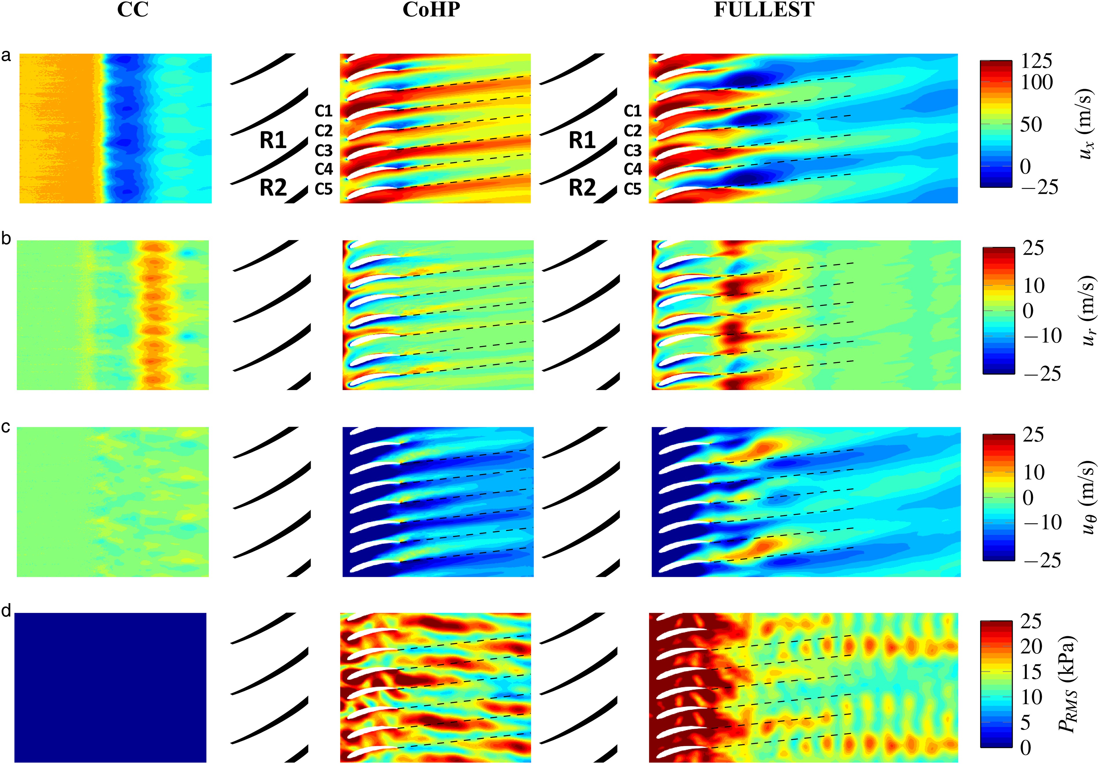
An axial cut at plane 31 (plane downstream of the axial diffuser) is shown in Figure 12 to illustrate the velocity components on the full height of the channel. As presented in Figure 11, the uniform velocity components in CC are not representative of the real conditions with the diffusers. Between CoHP and FULLEST, only
Figure 12.
Time-averaged velocity contours (cylindrical components) at plane 31 (trailing-edge of the axial diffuser) noted in blue in Figure 1 for (top) CC, (centre) CoHP and (bottom) FULLEST.

Figure 13.
RMS velocity contours (cylindrical components) at plane 31 (trailing-edge of the axial diffuser) noted in blue in Figure 1 for (top) CC, (centre) CoHP and (bottom) FULLEST.

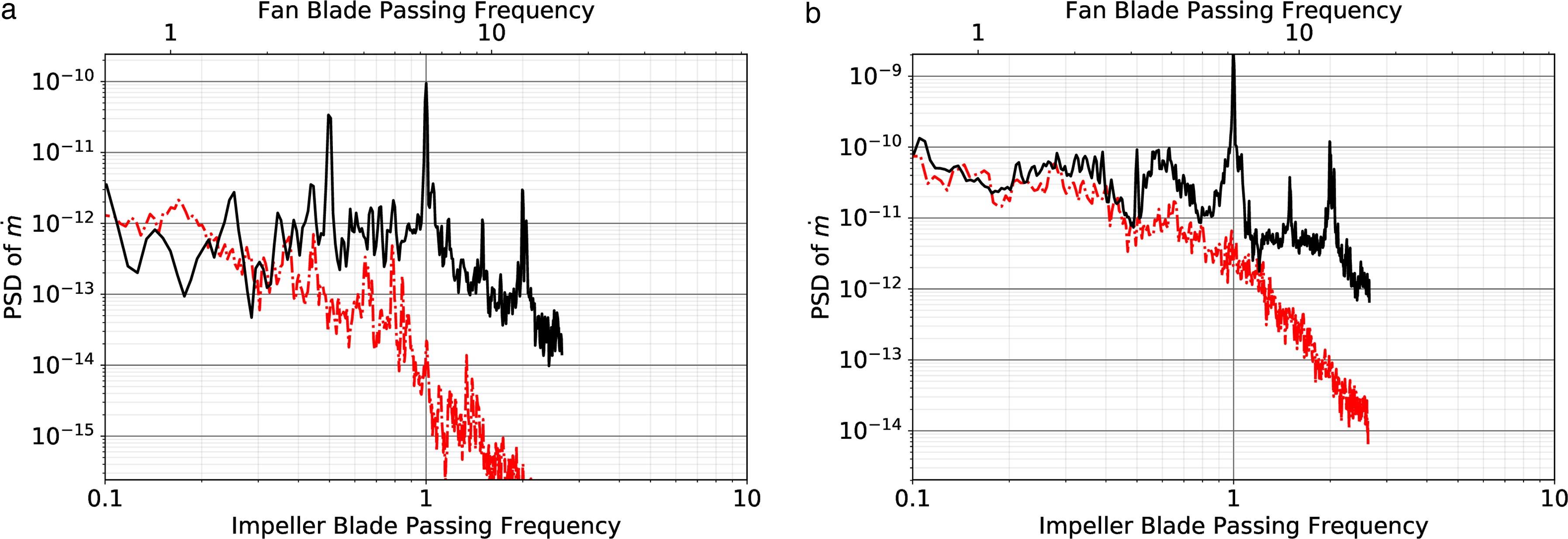
The flow then enters the flame-tube through the top and bottom dilution and primary holes; the swirlers farther back; and through the modelled multi-perforations of the flame-tube (Bizzari et al., 2018). In this case, each modelled perforation is set to either a constant suction or an injection of mass-flow rate at a determined temperature by the flame-tube side. The actual value of each perforation flow-rate is computed in a pre-processing step and does not change during the simulation. This means that with the actual modelling, and possibly contrary to real engines, the pressure fluctuations issued from the compressor cannot modify the mass-flow of each perforation. This is not the case for the dilution and primary holes or the swirler, which are meshed. The PSD of the mass-flow passing through the top primary hole and the swirler is shown in Figure 14. At low frequencies, both simulations achieve similar amplitudes. In FULLEST, the mass-flow entering the flame-tube fluctuates at the impeller BPF as well as harmonics and overall presents higher levels at high frequencies. This means that the pressure fluctuations incoming from upstream of the combustion chamber have an effect on the mass flow distribution of the dilution holes, and hence within the flame tube.
Figure 14.
Power spectral density (PSD) of the integral mass-flow rate m ˙
Inside the flame-tube, the time-averaged fields are barely impacted by the integration of the other components. This is illustrated by comparing the time-averaged static pressure, temperature and their RMS values for a meridional cut traversing the swirler in Figure 15. As expected, the most significant change comes from the pressure RMS as depicted in Figure 15b. As shown above, the pressure fluctuations propagate through the contouring casing of the combustion chamber. The same behaviour was reported by Pérez Arroyo et al. (2020) in an annular combustion chamber with a T-shaped vaporizer instead of a swirler. In FULLEST, the pressure fluctuations enter the flame-tube as can be seen by the higher levels of
Figure 15.
Mean and RMS contours at a meridional plane located at the centre of the swirler (top) CC and (bottom) FULLEST. (a) P (kPa). (b) P RMS T RMS
As shown in Figure 11, the angle at which the flow enters the contouring casing is different depending on whether or not the domain contains the axial diffuser. This change in
Figure 16.
Mean and RMS Mach number contours at axial planes (perpendicular to the axis of the machine) located at the primary holes. The observer is looking from the location of the fan.

Pressure fluctuations entering the flame-tube can be measured in the spectra at all locations. Figure 17 shows the spectra at four locations depicted in Figure 1 which correspond to a location where the gases are hot (Figure 17a), cold (Figure 17b) and at the exit of the combustion chamber (Figure 17c and 17d). The spectral content in the hot region has been substantially modified with respect to CC. In the stand-alone simulation, two broadband peaks arise at low and high frequencies. In FULLEST, the background amplitude is already higher than these peaks, specially at high frequencies. In addition to the peaks at the impeller BPF and harmonics, additional peaks are found at lower frequencies. Further analyses are needed to ascertain the origin of these supplementary peaks, which will be performed in the future with a longer simulated physical time to help for a better convergence of the low frequency range. In the cold region (Figure 17b), these peaks are masked by the background levels which are one order of magnitude above the levels in the hot region. The impeller BPF and harmonics are still visible in FULLEST and CC spectrum no longer presents broadband peaks and instead follows closely the spectrum in FULLEST. At the exit of the combustion chamber, some of the additional peaks are again visible in FULLEST since the background fluctuations have decayed. At this location, the impeller BPF peak is still about 4 orders of magnitude greater than the background. These fluctuations will be transported through the turbine stage and eventually radiate to the far-field. This peak and the first harmonic are also visible in the static temperature PSD as shown in Figure 17d, however, its impact on the performance of the turbine stage should be negligible since its amplitude is 2 orders of magnitude lower than the values obtained at the low frequency range. In CC, both pressure and temperature PSD present similar trends but without the tonal content.
Figure 17.
Power spectral density (PSD) at different locations noted in purple in Figure 1. (solid black) FULLEST, (dashed red) CC. (a) Hot region. (b) Cold region. (c) Exit of the flame-tube. (d) Exit of the flame-tube.
The exit of the combustion chamber (noted as plane 40) is further analysed in the following. This is a location of interest because it is also the inlet of the turbine stage (in the real engine). The information from this plane is commonly exchanged between design teams from the combustion and turbine departments and it is of crucial importance for the design of the turbine because non-uniform turbulence levels, residual swirl as well as temperature hot-spots may significantly impact the turbine life cycle (Dorney et al., 1999; Povey and Qureshi, 2009; Ireland and Dailey, 2010). Figure 18 depicts the contours at plane 40 for the time-averaged and RMS total pressure and temperature for both simulations. No difference is found for the time-averaged total pressure
Figure 18.
Mean and RMS total pressure and temperature contours at axial planes (perpendicular to the axis of the machine) located at plane 40 noted in orange in Figure 1 for (top) CC and (bottom) FULLEST. The observer is looking from the location of the fan. Black lines depict 1 sector of the combustion chamber centred on the plane of the swirler. (a) P t T t P t , RMS T t , RMS

Conclusions
The effects of the integration of several engine components is investigated with an integrated reactive large-eddy simulation with over 2,100 million cells of a 360 azimuthal degrees gas-turbine including the fan, radial compressor and annular chamber. This is performed by comparing the results against their stand-alone counterparts.
Even though there is no impact of the integration on the operating point of the machine (Pérez Arroyo et al., 2021), the average, RMS and spectra are greatly impacted by this process. This is clearly demonstrated by the rotating shock generated on the impeller leading edge at take-off conditions. The shock propagates upstream and interacts with the fan and OGVs. Stand-alone simulations of the fan component are not able to capture this phenomenon by construction unless better physical outlet boundary conditions are implemented. Note that the interaction between the high-pressure compressor and the fan can be deduced from the experimental spectra by Brown and Sutliff (2018). The shock is not only seen in the spectra but also affects the shape of the mean flow and RMS values. Indeed, turbulence generation on the fan blades and on the bypass duct, is modified as shown by the change in the position of the vortical structures in the fan wake, which some of them are excited at the frequency of the rotating shock. The authors recognise that the impact of the integration is enhanced by the fact that the engine is running at off-design conditions, however, it is at these operating points where LES could bring additional value since they are able to capture unsteady phenomena that may not be accounted for in the design process or with lower order models. Furthermore, the integration of the fan with the compressor generates a feedback on the compressor since the shock modifies the turbulence and background pressure fluctuations propagated from the OGVs into the impeller which highlights again the need of more realistic boundary conditions. The compressor itself is barely impacted by the integration and only the background pressure RMS increases in FULLEST. The integration of the combustion chamber deals with geometrical differences between stand-alone and FULLEST domains. Because the axial diffuser is not modelled in CC, the flow enters axially, which is not the case for FULLEST. At design conditions, the axial diffuser aims to realigning the flow with the axis of the machine. This is however not ensured for other operating points as shown in FULLEST. In this case, the difference in angle also affects the ejection angle of the jets generated on the dilution or primary holes and the angular position of the hot-spot that will impact the eventual turbine. The geometrical difference is not only the missing axial diffuser in CC but also the missing radial diffuser. The flow issued from the radial diffuser modifies the flow of the axial vanes and the flow that enters the contouring casing of the combustion chamber. Even though the effect of integration is minimal because the flow in the annular chamber does not directly enter the flame-tube, it could have an effect if the patterns align with the dilution and primary holes that connect with the flame-tube. Finally, integrating the combustion chamber with the compressor increases the spectral tonal content at all locations of the combustion chamber with peaks at the impeller BPFs and harmonics. This impact is though negligible for combustion as already demonstrated by Pérez Arroyo et al. (2020) in another configuration but may have detrimental consequences for the core-noise of the machine if the azimuthal content is modified (Boyle et al., 2020).
Finally, it is concluded that the study of integration effects of several components of an engine with LES is possible. The authors acknowledge that some effects of the integration are specific to this engine and simulation (i.e. the shock generated at the impeller and the lack of axial diffuser vanes in CC). Nonetheless, it gives a general idea of how non-physical boundary conditions often used in stand-alone simulations affect the flow. This work is a first step towards the LES of a full digital twin of the engine where effect of integration of the turbine stages and the exhaust jet are also considered.
Nomenclature
Symbols
Rotor chord length (m)
Peak at half the impeller BPF generated by the upstream propagating shock (−)
Normalised hub-to-shroud distance (−)
Mass-flow (kg/s)
Mach number (−)
Relative Mach number (−)
Static pressure (Pa)
Total pressure (Pa)
Static temperature (T)
Total temperature (K)
Normalised azimuthal angle with the azimuthal-sector angle (K)
Axial velocity (m/s)
Radial velocity (m/s)
Tangential velocity (m/s)