
Introduction
Aerodynamic design of gas turbines and jet engines relies on the assumption of infinitely accurate geometry and boundary conditions. Analytical models and CFD simulations are performed using these ideal conditions as input, as well as circumferential periodicity which assumes that all the blades are identical. However, the manufactured engine will always exhibit geometry variability due to the manufacturing process. The impact of this variability on the performance is of prior importance.
The variability of a compressor performance due to uncertain inlet total pressure profile has been tackled using probabilistic CFD (Gopinathrao et al., 2009) and Monte-Carlo simulation (Loeven and Bijl, 2010). Lavainne (Lavainne, 2003) used both deterministic and probabilistic simulations to investigate the effect of manufacturing tolerances on the performance of a compressor stage. He found out that variability in tip clearance has the strongest effect (when compared to chord, maximum thickness, leading edge and trailing edge thickness). More recently, the influence of geometric tolerances on performance have been studied both for turbines (Montomoli et al., 2011; Kolmakova et al., 2014) and for compressors (Lange et al., 2012; Liu et al., 2014; Ma et al., 2019). These works rely either on measurements of the blade geometry (Lange et al., 2012; Kolmakova et al., 2014; Ma et al., 2019) or on parametric studies (Montomoli et al., 2011; Liu et al., 2014).
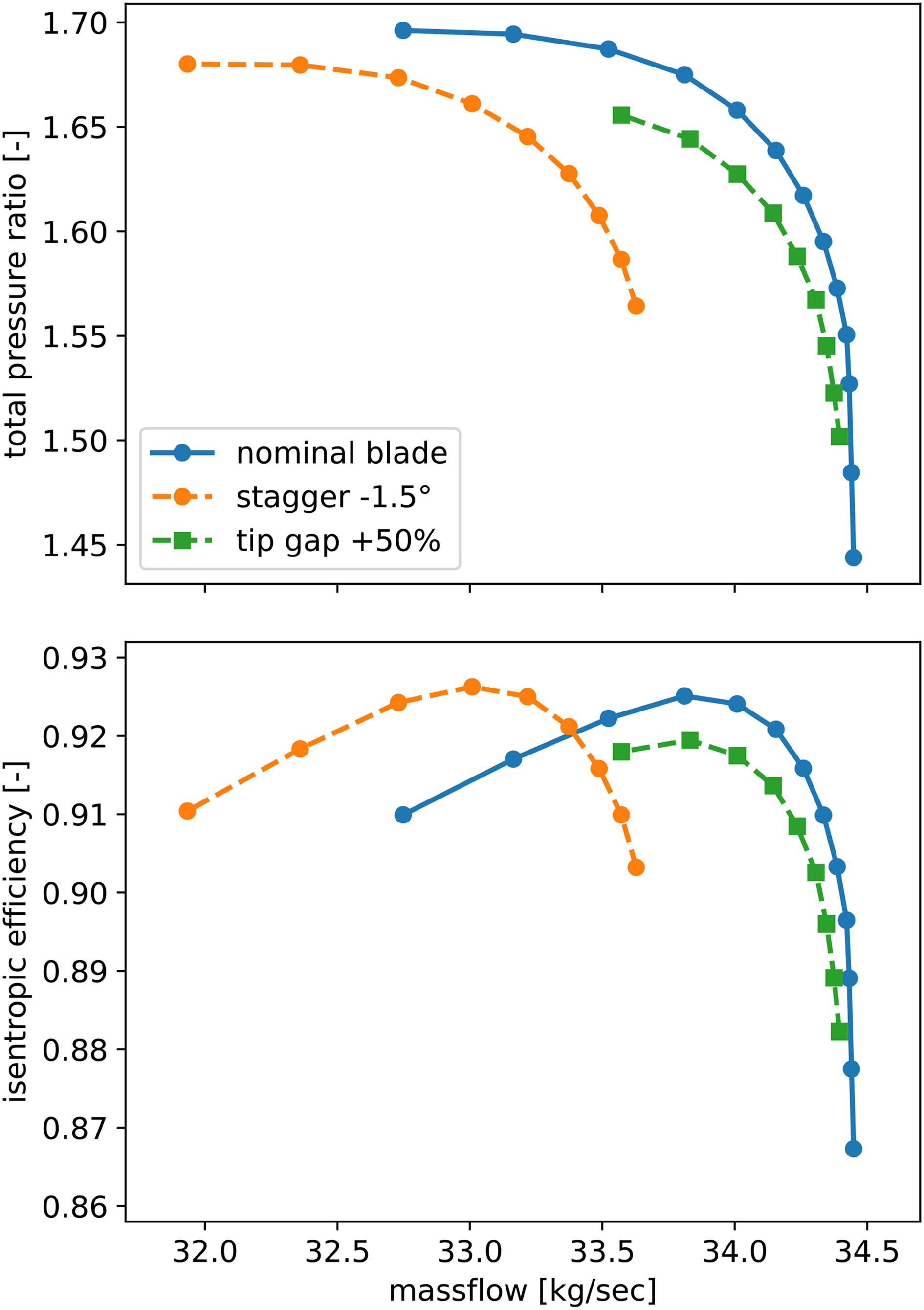
The behavior of a transonic compressor is mostly affected by variations of stagger angle (the angle between the blade’s chord and the rotational axis) and tip gap (the clearance between blade’s tip and the casing). The former influences the loading of each blade and the shock-wave position, which shifts the characteristic curve and affect the efficiency, while the latter is responsible for losses and secondary flows which trigger rotating instabilities. An illustration of the effect of stagger angle and tip gap variations on NASA Rotor 67 performance is shown in Figure 1.
Figure 1.
Effect of stagger angle and tip gap variation on NASA Rotor 67 total pressure ratio and isentropic efficiency.
Once assembled in a rotor assembly, blades with geometry variability lead to a degradation of performance. This is due to the average effect of geometrical tolerances and to the variation between adjacent blades. In other words, the order in which the blades are arranged influences the performance, as shown in previous work (Suriyanarayanan et al., 2022).
In the first design steps, the main concern is not the optimal arrangement but the uncertainty quantification of the compressor performance. Full-annulus numerical simulations can be used in industry to assess the behavior of a specific arrangement but are computationally prohibitive to evaluate thousands of them. To overcome this, a surrogate model has been developed in this work. It relies on physical insights and meta-modelling to greatly reduce the computational costs. Most of the physical phenomena are captured thanks to inexpensive single-passage and double-passage computations. The model, which can quickly output a performance curve for a given set of blade, can then be used for the uncertainty quantification study.
In the first part of the paper, the flow solver, the test cases and the different blade arrangements are presented. The surrogate model for stagger angle and tip gap variation is then described and validated against CFD data. Finally, the model is used to perform an uncertainty quantification of compressor performance due to manufacturing tolerance.
Methodology
In this section the numerical models, the test cases and the blade arrangements are presented.
Flow solver
The simulations were performed using the in-house CFD solver AU3D, developed at Imperial College London-VUTC over the last 30 years. AU3D is a three dimensional, time-accurate, viscous, compressible Reynolds Averaged Navier-Stokes (RANS) solver that uses Spalart-Allmaras (SA) model to evaluate the turbulent eddy viscosity. The solver operates on a semi-structured mesh with hexahedral elements found around the airfoil and prismatic elements in rest of the passage. The boundary layer region in rotor-to-rotor grid has a body-fitted O grid while rest of the region is unstructured. The tip clearance geometry is meshed by triangulating the blade tip and mapping extra layers over the tip (Sayma et al., 2000). The flow solver is based on vertex-centered finite volume method. Inviscid fluxes are discretised by JST central scheme with matrix artificial dissipation and a pressure switch in the vicinity of discontinuities. The resulting system of equations is advanced in time using an implicit scheme with Jacobi iteration and dual time stepping. The solver has been successful in predicting the design and off-design conditions of turbomachinery (Vahdati and Imregun, 1996; Dodds and Vahdati, 2015; Lee et al., 2018).
Test cases
Two different fans are considered in this study. The first one is NASA Rotor 67 (Strazisar et al., 1989), a highly tip loaded fan for which lots of experimental and numerical data is available. The second one is a wide chord fan representative of modern engines. The characteristic features of the two test cases are shown in Table 1.
Table 1.
Comparison of test cases (design point).
| NASA Rotor 67 | Wide chord fan | |
|---|---|---|
| Number of blades | 22 | 18 |
| Rotational speed | 16,043 rpm | 12,650 rpm |
| Pressure ratio | 1.63 | 1.26 |
| Massflow | 33.3 kg/sec | 36.7 kg/sec |
| Tip gap | 0.6 mm | 0.9 mm |
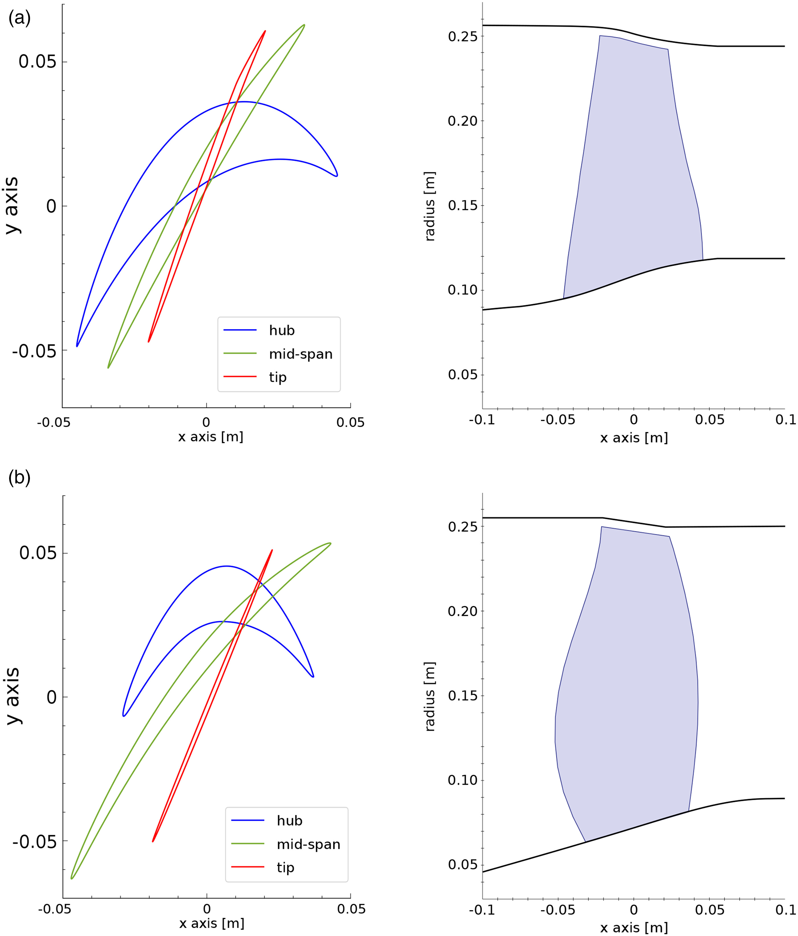
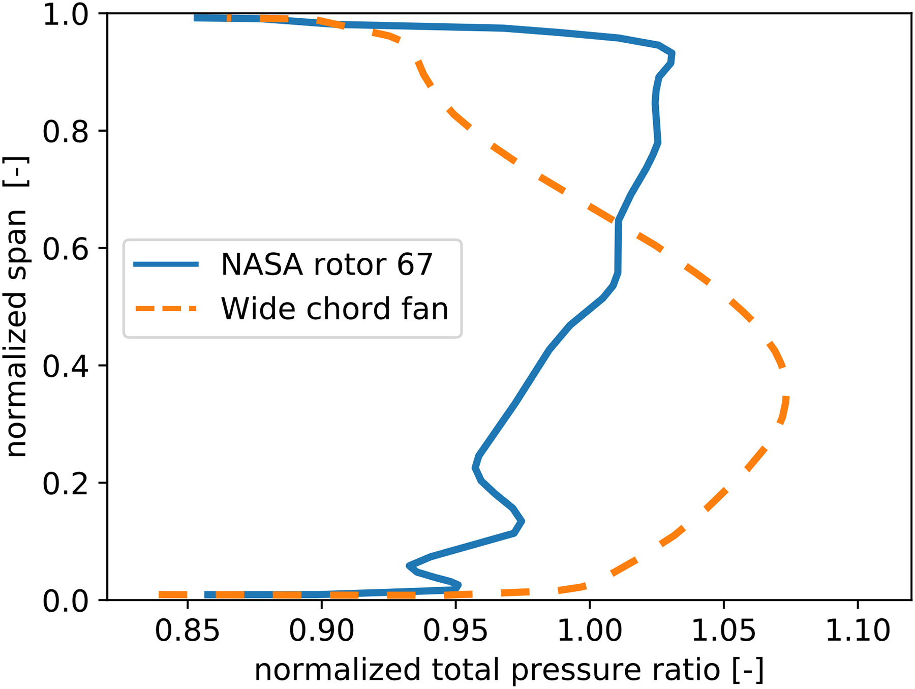
To visualize the differences between the two test cases, a meridional view and the airfoils at hub, mid-span and tip sections are plotted in Figure 2a for NASA Rotor 67 and in Figure 2b for the wide chord fan. The hub to tip ratio is smaller for the wide chord fan, which is typical of high by-pass ratio fan which rely on large massflow and low rotational speed to produce thrust. The radial profile of total pressure ratio (normalized by its value at design point) is shown for both test cases in Figure 3. The maximum pressure ratio is obtained at the tip for NASA Rotor 67 and around 40% span for the wide chord fan.
A mesh size of 1 million points per passage was used for both the test cases based on a mesh convergence study. Single, double passage, and full annulus computations will be used. For all these cases, total pressure, total temperature and flow angles are specified at the inlet boundary. Downstream of the rotor, there is a convergent nozzle and the outlet where low back-pressure is imposed. Thus, the nozzle is choked and ensures that disturbances from the exit do not propagate upstream (Vahdati et al., 2005). To generate the characteristic curve at a given speedline, from choke to stall point, the downstream nozzle is gradually closed, reducing the massflow.
To represent stagger angle manufacturing tolerances, a twist is imposed to the blade by using mesh morphing. Following previous work (Suriyanarayanan et al., 2022), the variation of stagger angle is in the range of ±1.5°. The tip gap variations do not impact the performances of the wide chord fan which is not tip-loaded (see Figure 3). Therefore, only NASA Rotor 67 will be considered. Five meshes have been generated with five different gaps, ranging from 0.3 to 1.5 mm (50% to 250% of nominal tip gap).
Blade arrangement
Blades with manufacturing tolerance are, by definition, no longer identical. As a consequence, given a set of manufactured blades, the arrangement may have an impact on compressor performance. For any geometric feature
Given a set of N blades with different values for
Surrogate model
The goal of the surrogate model is to output the characteristic curve of a compressor at a given rotational speed knowing the blade distribution. An example is shown in Figure 5 for a 6 blades rotor with three different blade geometry (tip gap or stagger variation). First, one has to choose a blade arrangement. Without loss of generality, a symmetric pattern has been used to simplify the example. Once the input (i.e. an ordered blade distribution) is defined, the model sweeps through each pair of adjacent blades and computes the characteristic curve of an equivalent compressor, consisting of these two blades arranged in an alternated pattern. An exact solution can be achieved by using double passage simulations with periodic boundary conditions, or by using meta-modelling from a sample of CFD solutions. To obtain the performances of the targeted blade arrangement, the equivalent compressors characteristic curves are mass-averaged. Formally, the massflow
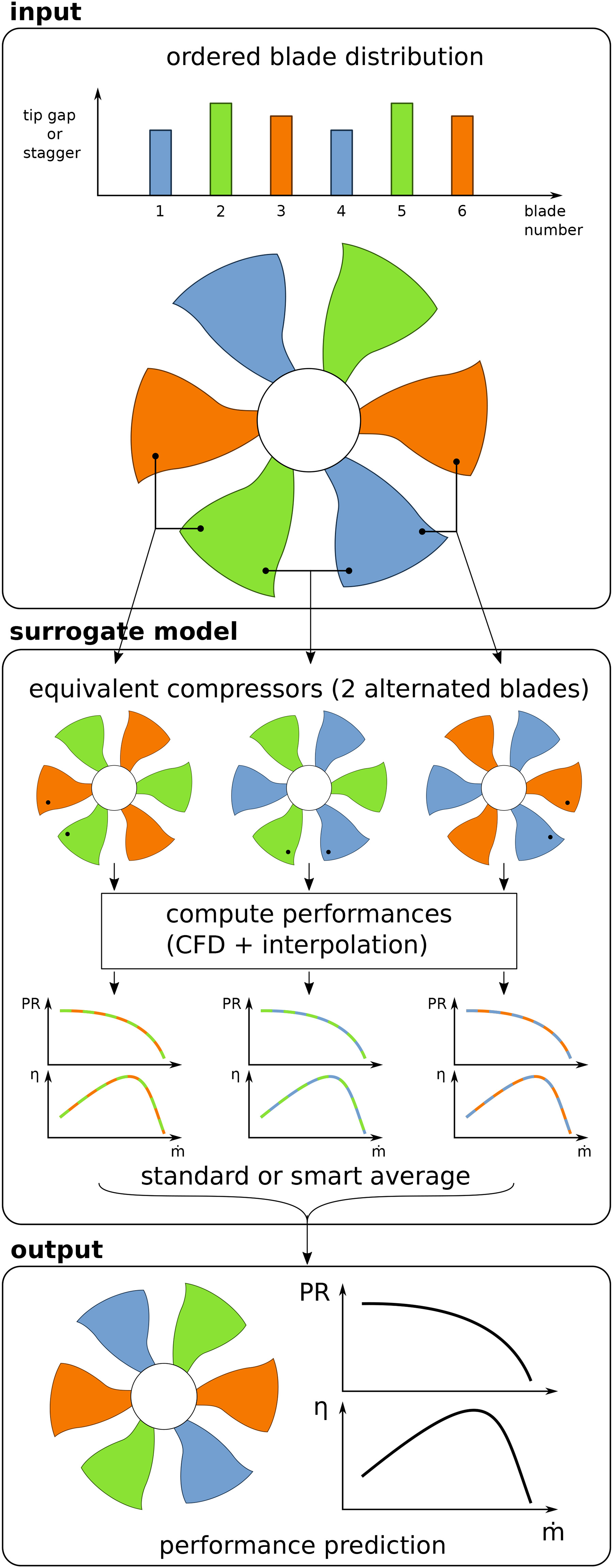
where N is the number of blades,
This strategy allows the model to compute the effect of the blade i on itself and its neighbors (
Previous work (Suriyanarayanan et al., 2022) has shown that tip gap variations affect both stall margin and performance whereas stagger angle variations mostly affect the latter. While relying on the same strategy, two independent surrogate models are needed to compute the characteristic curve of equivalent compressors (see the middle-part of Figure 5).
Stagger angle variations
Concerning stagger angle, the surrogate model must take into account two effects. The first one is a shift in average stagger angle. If the input is a set of identical blades at a stagger angle different from the designed geometry, the incidence would change and the characteristic curve would shift. This effect can be accurately modelled by single-passage computations with different stagger angle. Characteristic curves are computed for different stagger angle and linear interpolation is used to recover any value of average stagger angle. Figure 6a shows how to recover an angle of 0.34° for instance.
Figure 6.
Interpolation strategy for stagger angle variations. (a) average stagger angle (single passage CFD). (b) adjacent mis-stagger (double passage CFD).
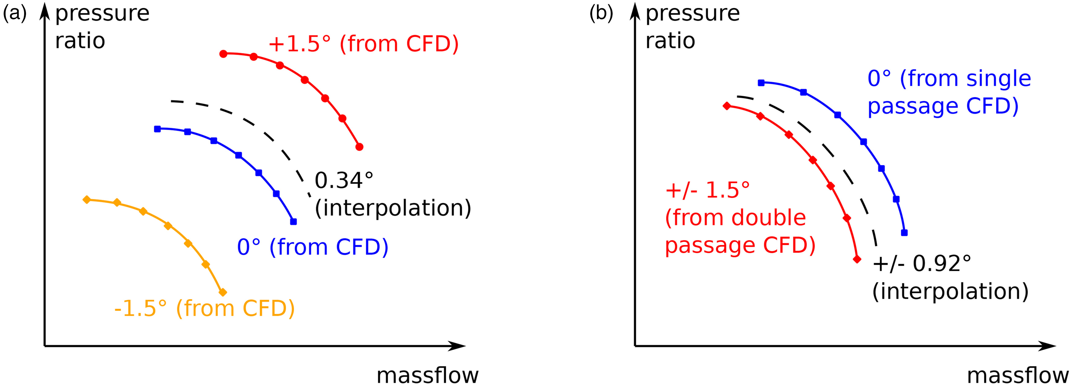
Once the average stagger angle is correctly modelled, one needs to introduce the effect of stagger variation between two adjacent blades, which we will call adjacent mis-stagger. This effect can be estimated by running double passage computations, which represent a rotor with two sets of blades arranged in an alternated pattern. Keeping the average stagger angle constant (for instance 0°, which corresponds to the designed geometry), one can isolate the effect of adjacent mis-stagger. Using double passage computations, it is possible to reconstruct the effect of any adjacent mis-stagger by interpolation, as shown in Figure 6b with 0.92° for instance.
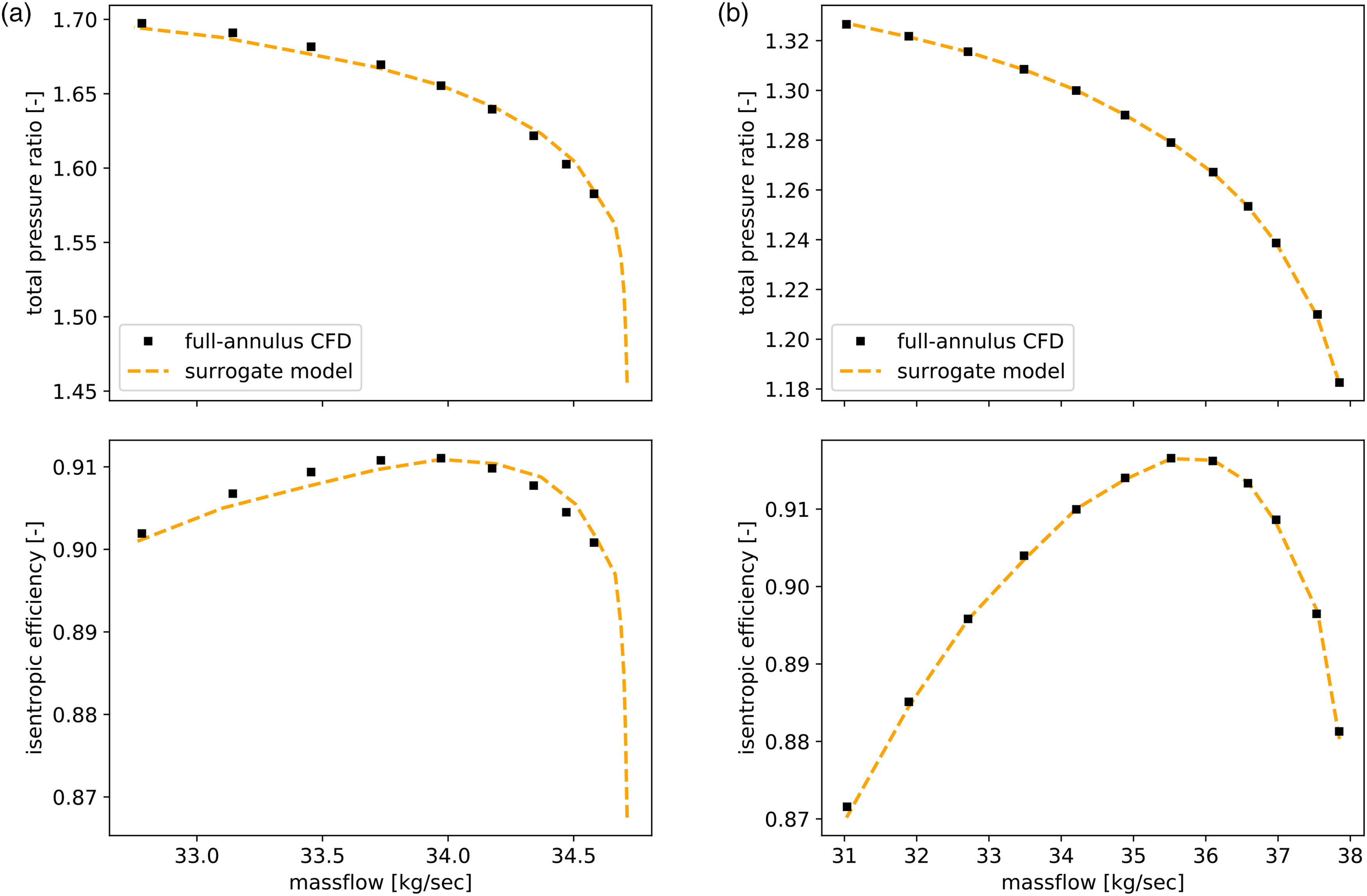
A convergence study has been done to evaluate the number of points needed to achieve a satisfactory interpolation. The comparison of predicted total pressure ratio with full annulus computations is shown in Figure 7a for Rotor 67 and in Figure 7b for the wide chord fan. 5 single passage computations (−1.5°, −1°, 0°, 1°, 1.5°) and two double passage computations (±1° and ±1.5°) were choosen, yielding a maximum error on total pressure ratio of
Tip gap variations
Tip gap variations quickly lead to non-linear effects on stall margin and performance. In that case, simple linear interpolation did not prove sufficient to build a reliable surrogate model. To overcome this issue, free parameters have been added in the averaging process. The resulting formula, which is referred as smart average, is given by
Using full-annulus computations as target values, the parameters are computed using a non linear least square optimization. Concering the performance prediction, it is more effective to work with a scaled total temperature ratio rather than with isentropic efficiency. Indeed, total pressure ratio curve is monotonic while isentropic efficiency curve exhibits a maximum at design point. The two curves cannot be superimposed, a different set of parameters would thus be needed for each of them, increasing the need of training data. On the other hand, we know that for isentropic transformation,
The curve of total temperature ratio raised to the power
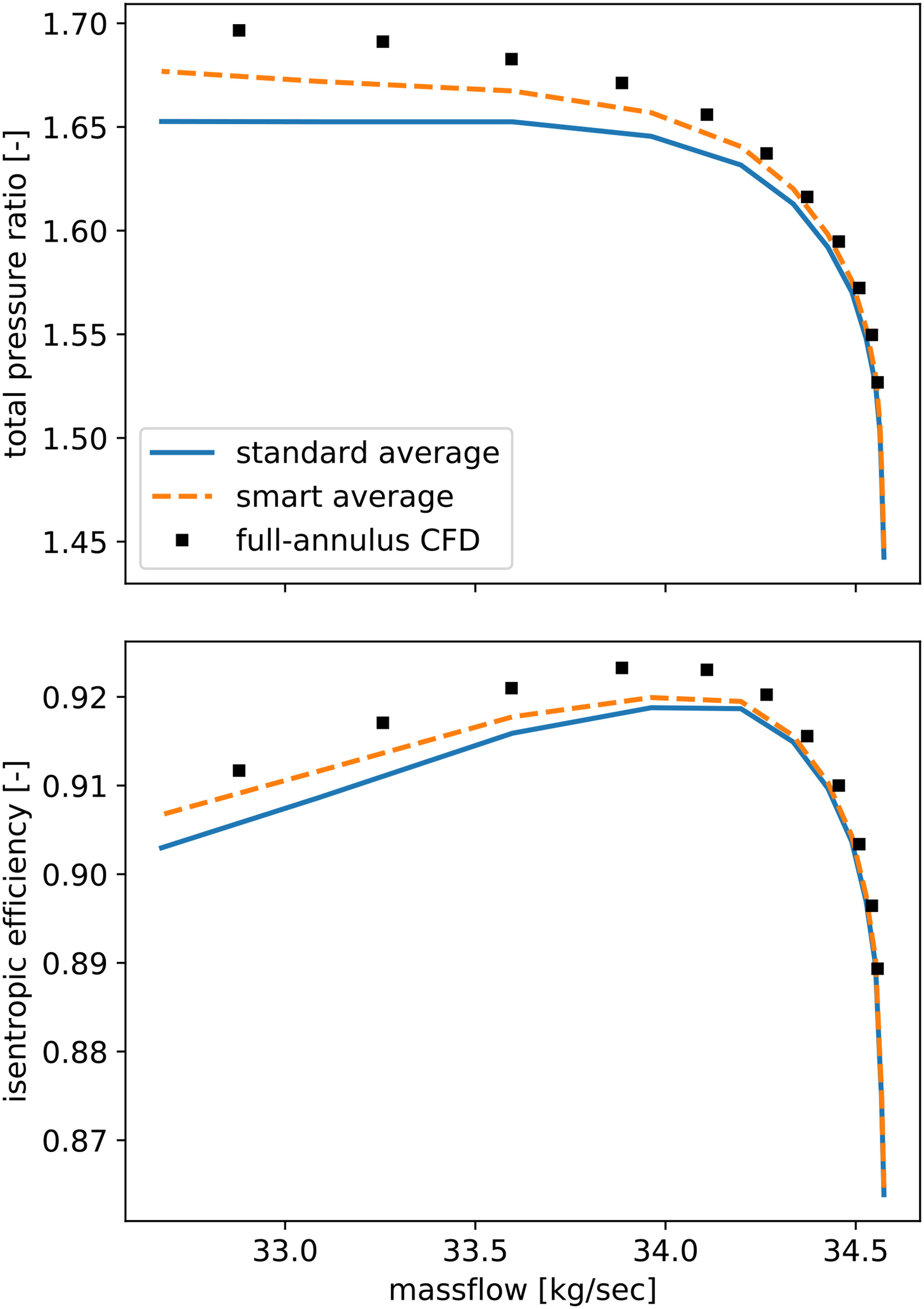
A comparison of standard and smart average with full-annulus CFD is given in Figure 8. The maximum relative error on total pressure ratio is
Figure 8.
Comparison of standard and smart average surrogate model with full-annulus CFD for NASA Rotor 67.
This section presented the strategy of the surrogate model used in this paper for stagger angle and tip gap variations, as well as its validation against CFD data. In the next section, the surrogate model will be used to investigate the impact of manufacturing tolerance on performance.
Uncertainty quantification
Uncertainty quantification can be used to assess the variability of a design with respect to manufacturing tolerance. Using manufactured blades, one can compute the range of these tolerances and their distribution (gaussian, uniform, …). In this work, we consider uniform continuous distribution of stagger variations between
To ensure that all the design space is spanned, 50,000 sets of blades are generated. Each set can then be assembled in any order, resulting in one rotor configuration (we assume that the structural dynamic balancing is done afterwards and do not constrain the choice of blade arrangement).
Previous work (Suriyanarayanan et al., 2022) showed that stagger angle variations create a change in passage geometry and incidence angle which induce a displacement of the shock-wave. The maximal efficiency is obtained, by design, for a specific shock-wave position which is, by symmetry, the same for all passages. Mis-stagger between adjacent blades breaks the annular symmetry and creates a displacement of the shock-waves, leading to a less efficient configuration. Hence, to maximize compressor performance, one needs to minimize adjacent mis-stagger. This is achived thanks to a sinusoidal pattern.
For a set of blades with identical tip clearance at peak efficiency, each blade generates its own leakage flow. When getting closer to stall, the leakage flow of adjacent blades can merge and create rotating stall cells, breaking the annular symmetry (or at least reducing the wave-number of the periodic pattern). To maximize the compressor performance, one needs to contain the leakage flow of each blade. Given a blade with a large tip clearance, placing a blade with small tip clearance right after it will stop the leakage flow. Hence, to maximize compressor performance, one needs to maximize adjacent tip-gap variations. This is achieved thanks to a zigzag pattern. More details on these two mechanisms can be found in (Suriyanarayanan et al., 2022).
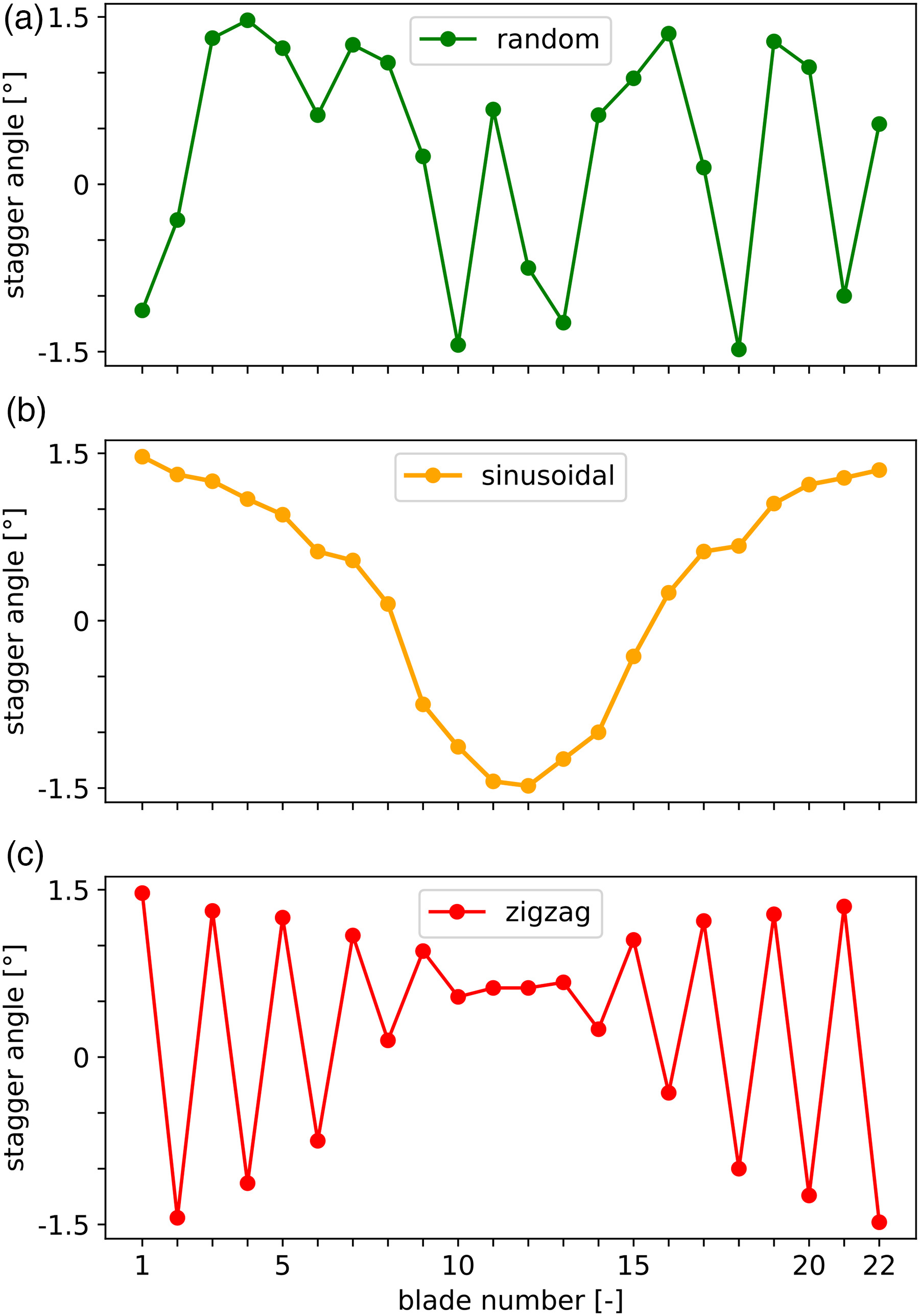
The surrogate model allows us to arrange each set of blades along any pattern and to plot the resulting performance envelope. This work focuses on three arrangements: sinusoidal, zigzag and random (which can be considered as baseline).
Stagger angle variations
The effect of stagger variations on maximum isentropic efficiency is plotted in Figure 9a for Rotor 67 and in Figure 9b for the wide chord fan. As expected, the worst performance is given by zigzag arrangement while the best one is obtained using the sinusoidal pattern. More interestingly, the range of efficiency depends on the chosen arrangement.
Figure 9.
Envelope of maximum isentropic efficiency against average stagger angle for three different arrangements. (a) NASA Rotor 67 (b) Wide chord fan.
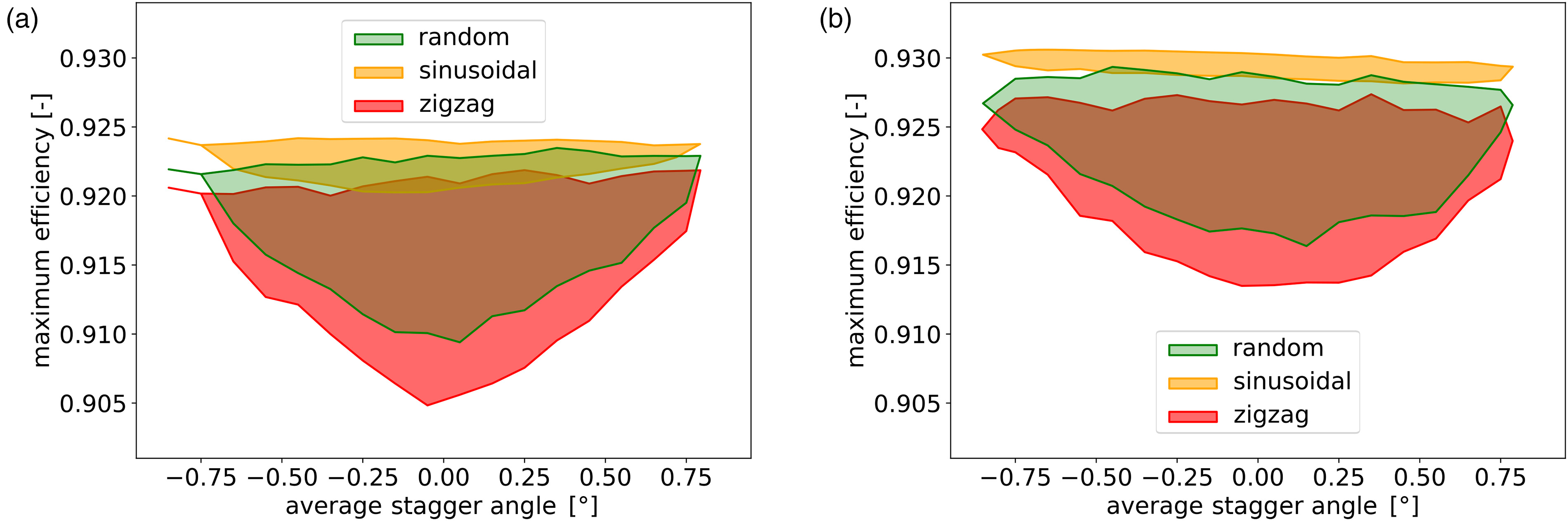
For Rotor 67 and the wide chord fan, arranging the blades in a sinusoidal pattern guarantees that narrowest envelope, whereas it is widest for the zigzag pattern. This is clearer when looking at the probability density function against average stagger angle, plotted in Figure 10 for Rotor 67. It shows that the maximum isentropic efficency fits in the range
Figure 10.
Distribution of maximum isentropic efficiency for different blade arrangements on Rotor 67.
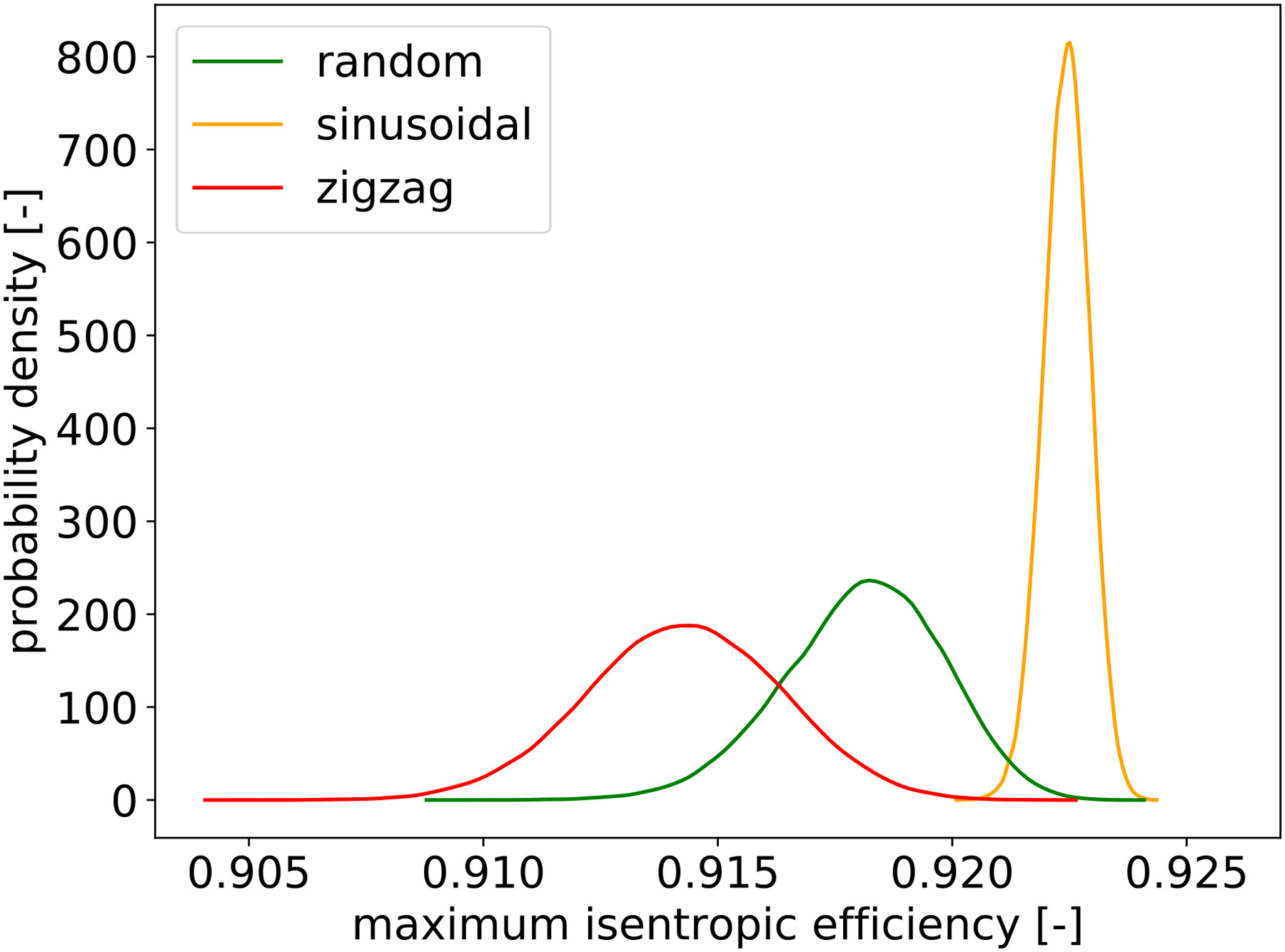
While these two configurations are representative of the best and the worst case, random arrangement has also been evaluated. It is representative of a process where no arrangement strategy is choosen or where information on manufactured blade geometry is not available. The width of the envelope for random arrangement is similar to the zigzag arrangement envelope, indicating large variability.
Tip gap variations
By its design, which maximizes the loading at mid span, the wide chord fan is insensitive to tip gap variations. Hence, only Rotor 67 will be used in this section to evaluate the effect of tip gap variations on performance.
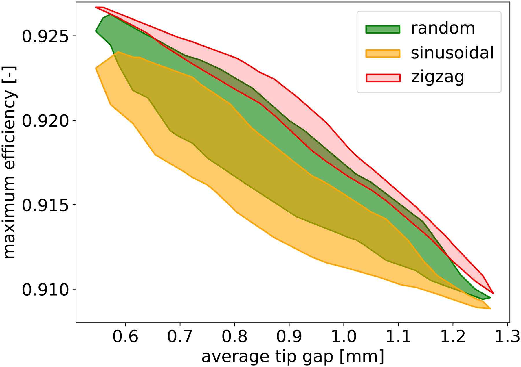
The effect on maximum isentropic efficiency is plotted in Figure 11. As expected, a general trend with negative slope is observed, reflecting the increase in losses when the tip clearance opens. The best and worst performances are associated with zigzag and sinusoidal pattern respectively, which confirm previous work. Similarly to the uncertainty quantification study on stagger angle variations, the envelope width is small for the best arrangement and large for the worst one. Random arrangement gives in-between performances but variability as large as the worst arrangement.
Figure 11.
Envelope of maximum isentropic efficiency against average tip gap for different blade arrangements.
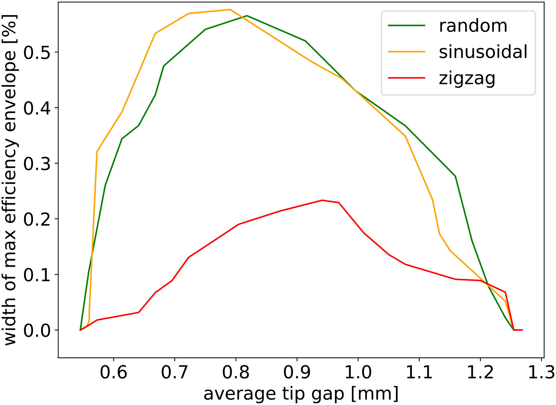
To further investigate and to quantify the variability of efficiency with respect to different arrangement, the vertical width of the maximum efficiency evelope is plotted againt average tip gap in Figure 12. For an average tip gap equal to 0.9 mm, the envelope is twice as wide for sinusoidal and random arrangement, when compared to zigzag. This indicates once again that the arrangement yielding best performance is associated with the lowest variability.
Figure 12.
Vertical width of maximum isentropic efficiency envelope against average tip gap for NASA Rotor 67.
To conclude, it has been shown that the arrangement yielding best performance (sinusoidal for stagger angle and zigzag for tip gap) also yields the lowest variability. The variability largely increases if the blade arrangement is not considered or, equivalently, if the manufactured blade geometry is not measured. This shows the paramount importance of manufacturing tolerance assessment and blade arrangement on compressor performance.
Future work
To the best of author’s knowledge, this is the first attempt at building a surrogate model to predict performance of a compressor with manufacturing tolerance. In future work, the model will be used to investigate the effect of tip gap variations on stall margin. Compressors with both stagger angle and tip gap variations will also be studied. Stagger angle variations can also lead to mistuning, which impacts the aeroelastic behavior of the rotor (Stapelfeldt and Vahdati, 2018). The uncertainty quantification of the flutter boundary with respect to stagger angle variations is thus another field of interest.
Conclusions
This work investigated the influence of manufacturing tolerance on compressor performance (total pressure ratio and isentropic efficiency). To quickly evaluate the characteristic curve of a compressor given of set of manufactured blades, a surrogate model has been developped. It relies on the physical assumption that most of the effect is on the blade itself and its neighbors, whereas the influence of further blades can be neglected. This allows to build an efficient model using few single-passage and double-passage computations, which are inexpensive. For stagger angle variations, performance can be predicted with a maximum error of 0.2%. For tip gap variations, which are highly non-linear, the maximum error is 1.3%. To achieve this, an extra step called smart average is needed, which optimizes a set of parameters using few full-annulus computations.
Given the good agreement of the surrogate model with CFD data, it has been used to investigate the effect of blade arrangement on 50,000 sets of manufactured blades. For each set, three arrangements have been studied:
random, which is representative of not measuring blade geometry
sinusoidal, which minimizes the variation between two adjacent blades
zigzag, which maximizes the variation between adjacent blades
These results were obtained on two very different rotor designs and are thus expected to be general. They may however depend on the range and the distribution (normal, gaussian, …) of the manufacturing tolerance. Following the methodology described in this work, one can build their own surrogate model. The performance variability can then be assessed by using the company’s own data on manufacturing tolerance.