
Introduction
Novel aircraft engines, such as the ultra high-bypass aircraft engines, will play a crucial role in the future development and increased efficiency of modern aircraft Merkl (2016). Since the performance and, above all, the economy of an aircraft are directly and inextricably linked to the performance of the aircraft engine, constant efforts are being made to increase both the thrust generation and the fuel efficiency of engines. These continuing demands for more power and less fuel consumption ultimately lead to new and modern engine architectures that work even closer to the aerodynamic, thermal, and structural limits of the various components of the whole jet engine von der Bank et al. (2014).
However, the resulting design optimisations and modifications (e.g., 3D optimised blades) lead to more complex parts and functional integration within a part or assembly and thus also to an increasing sensitivity in geometric variations. Due to the high degree of interactions between the components and between individual parts within the components, geometry deviations that occur due to manufacturing and repair tolerances, as well as deterioration (e.g., erosion), can have a much greater impact on efficiency and performance than in previous generations of aircraft engines. Lavainne (2003) describes the geometry variations of compressor blades and names typical production scatter in the order of up to 1.5% in the chord length, 0.8% in the leading or trailing edge thickness, and 2.5% in stagger angle. Particularly in the case of modern aircraft engines, where experience and data are not available, knowledge-based approaches that investigate the influence of geometric variances on the overall system are essential.
Therefore, in Reitz et al. (2018) a virtual process for geometric evaluation of compressor blades was developed to determine the influence of geometry variations. Using measured compressor blades, high sensitivites of the loss coefficient and efficiency to aerodynamic blade parameters such as camber and stagger angle were identified.
Furthermore, Bammert and Sandstede (1976) already investigated the effects of manufacturing tolerances on the performance of turbines. For example, the enthalpy decreased by 15%, mass flow increased by 15%, and efficiency of the axial turbine fell by 1.4% when the blade thickness was reduced for the first two stages of a four-stage axial turbine. A thickening of the last two stages of the same turbine, on the other hand, causes an increase in the enthalpy gradient by 6% and a drop in the mass flow by 6%. The efficiency drops disproportionately by 3%. In Schwerdt et al. (2017), investigations were carried out on worn and factory-new first-stage turbine rotors. For this purpose, both blades were digitised using a 3D laser scanner, built up as a numerical model and numerical simulations were carried out. In the evaluation, differences were detected in the pressure and temperature field on the blade surface of the examined blades.
Based on the production and deterioration as well as repair influences, there are no exactly identical blades; each blade has its own individual parameter combinations within the permissible production tolerances. Consequently, each blade has individual aerodynamic properties. Numerical analysis of each individual blade is not practical, rather, probabilistic studies are used for simple analysis of the individual parameters. In Scharfenstein et al. (2013), 500 blades were digitally measured and evaluated. For this purpose, the three-dimensional geometry was reduced to two-dimensional sections and completely described by means of 14 blade parameters (Heinze et al., 2014). With the help of these determined parameters, it was possible to set the limits for the random generation of the samples, which were used in a Monte Carlo simulation. A sample of 50 blades showed that there is a strong dependence of the reduced mass flow and reaction degree on the stagger angle, as well as a strong dependence of the efficiency to the trailing edge thickness. A similar probabilistic approach was used by Ernst et al. (2016) for analysing a data set containing of 20 measured low-pressure turbine (LPT) blades that showed significant geometric variations due to operation. The probabilistic simulations with 100 samples were performed for several operating points that showed a strong dependency on the chosen operating point. The polynomial-based sensitivity analysis identified the stagger angle and the trailing edge thickness as the most important parameters for the change in aerodynamic efficiency.
In Gilge et al. (2019), real surfaces of worn compressor blades of a conventional high-bypass turbofan were measured and evaluated. The variations can be seen both in the roughness height (quantified by the roughness parameters) and qualitatively in the shape of the roughness structures. These structures are oriented at an angle of 45° to 90° perpendicular to the flow direction and are caused by oil and flow particles.
In Seehausen et al. (2020), the obtained roughness information was transferred to a CFD model of the V2500-A1 high-pressure compressor and the effect of complex surface structures on the overall compressor performance was evaluated. The simulations with stage roughness variations show that the first stage has the greatest impact on compressor performance. Furthermore, the surface roughness influences the narrowing and displacement of the compressor maps to a high degree, thereby decreasing the pressure ratio much more significantly than the capacity and efficiency in all speed curves considered. In general, these studies show that geometry variations and surface roughness have a significant influence on the integral pressure ratios
In Goeing et al. (2020a), the findings of the roughness study already discussed were transferred into a whole aircraft engine performance simulation program and their effect on the overall performance was analysed at various steady-state operating points and transient manoeuvres. It was shown that the exhaust gas temperature is increased by more than 20% at steady-state operating points and transient temperature loads by up to 30%. Furthermore, combined deterioration of high-pressure compressor (HPC) and HPT was investigated in Goeing et al. (2020b). The characteristic effects of the investigated deterioration on performance can be summarised as follows:
SFC and Tt5 can be used to determine the degree of deterioration.
Temperature downstream the combustor (Tt4) and the rotational speeds in combination can be used to identify the components affected by the deterioration.
The distance to the stability limit in the HPC and the deviation between the transient and steady-state operating lines differ significantly for HPT and HPC deterioration.
Both HPC and HPT degradation have significant influences on the global engine behaviour, but HPC degradation has a significantly stronger effect on the stability of the engine.

In this work, the developed process is demonstrated using the first stage of the HPT blade of the V2500 turbofan engine as an example in a high Technology Readiness Level of 7. The V2500 turbofan with low-pressure compressor (LPC), intermediate-pressure compressor (IPC), HPC, HPT, LPT, and a common thrust nozzle, from IAE (International Aero Engines) typically powers the Airbus A320-100 representing medium-range aircraft. The paper discusses first how the blades used are digitised, parameterised and reconstructed automatically for an automated meshing process. Subsequently, the CFD set-up and the performance simulation are outlined, and both, the sensitivity analyses and the metamodels employed are presented. A DoE is carried out to quantify the global sensitivities of geometry variations and aero-thermodynamics. Finally, the virtual process is run on the best and worst HPT blades to illustrate the influence of isolated and combined module variances on the performance. This combines the different methods for evaluating local aerodynamics and global performance, providing a knowledge-based process that examines the causalities between component variations and performance changes from the bottom up.
Methodology for the evaluation of the virtual twin of the aeroengine
In this chapter, the single steps of the virtual process for a component evaluation are discussed (see Figure 1). The virtual analysis is carried out on the example of the first HPT rotor stage blade of the V2500-A1. Based on the IFAS research aircraft engine, performance data of the V2500-A1, information, and geometries of the HPT, which are necessary for a CFD set-up, are available. In order to develop the real repair process in CRC 871 (Aschenbruck et al., 2014), a large number of HPT-blades were required. This high number could not be provided by the V2500-A1, so the repair process was developed on scraped HPT-blades of the V2500-A5.
Digitisation of HPT blades
A fringe projection system is used (Betker et al., 2020) for the digitisation of the blade geometry. In order to automate the process and reduce systematic errors, the projector and camera of the measuring system are positioned with a serial robot (see Figure 2). The projector projects an alternating stripe pattern on the scraped and heavily deteriorated blades to measure the geometry from root to tip. The camera captures the deflection of the stripes. A measuring computer calculates the distance to the camera from these images and creates a point cloud from it. With a high dynamic range measurement, blades with different optical surface properties can be measured.
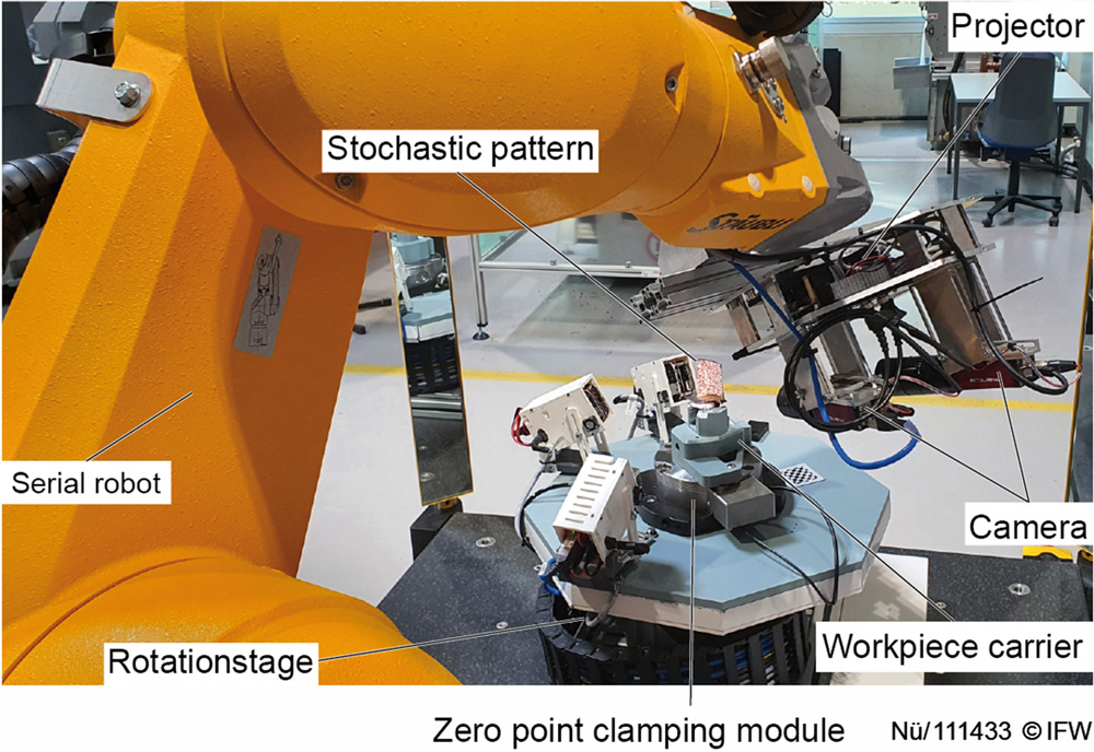
The blade is clamped using a workpiece carrier and a zero point clamping module, that is mounted on a rotation stage. On this stage, three projectors are mounted and project a stochastic pattern on the blade. This pattern, overlapping measurements, and the special geometry of the workpiece carrier are then used to merge the point clouds of the 13 single measurements to a combined point cloud.
The coordinate system of the measurement system is calibrated once with a normal. Because of the low absolute accuracy, as well as the assembly tolerances of the workpiece carrier, the position and orientation of the measured blade varies in the fixed coordinate system. An iterative closest point algorithm aligns the worn blade to a reference blade to determine the parameters of each blade on the same positions. After the alignment, blade slices of 1.2 mm around the planes that are used in the next steps are extracted and parameterisation (±600 µm) are extracted and converted into a 3D-model with surfaces. Additionally, a convex hull is used which allows the robust closing of holes from heavy damage and cooling air holes.
The alignment is performed by an Iterative Closest Point Algorithm. The alignment is carried out globally, since individual geometry parameters are not sufficient due to the geometry variations. Due to the strong wear in the blade tip, the alignment is only used in the range from the foundation to 5 mm below the blade tip. The iteration is converged if the change is less than 3 micrometers or 30 iterations are exceeded (Nübel and Denkena, 2022).
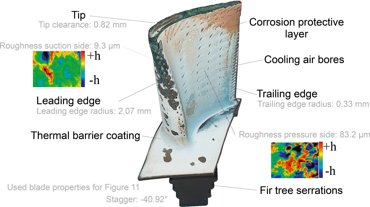
After the marcrosopic geometric properties of the investigated blades, the small-scale surface structures are optically measured with a con-focal laser scanning microscope (Keyence VK-X200). In the process, the measurement of surface roughness is performed at five positions on the suction side and at four positions on the pressure side at mid-span with a 20× magnification lens. For CFD simulations an equivalent sand-grain roughness
Parameterisation
The digitised blade is analysed in 20 different blade sections at constant radial positions based on the slices from the digitisation. Each blade section is parameterised by algorithms based on Heinze et al. (2014) and Ernst et al. (2016) and exemplified in Figure 3. The camber is approximated by the Delaunay triangulation (Aurenhammer, 1991), where the middle points of enveloping circles around the Delaunay triangles correspond to the camber line. This approach fails near regions with high curvature, e.g. leading- or trailing -edge. Therefore, different filters, based on the curvature of the camber, are applied in regions near the trailing- and the leading-edge in order to remove outliers. The leading-edge camber is approximated by a second order function attaching to the estimated camber based on the Delaunay triangulation and the trailing-edge by a first-order function, resulting in crossings with the blade´s macroscopic geometry. These crossings are the leading-edge and trailing-edge stagnation points which are used for rotating the blade around the origin and shifting the profile that the leading-edge stagnation point is placed at the coordinate system´s origin and the trailing-edge is horizontally aligned with the origin. This simplifies further calculations. The leading-edge radius
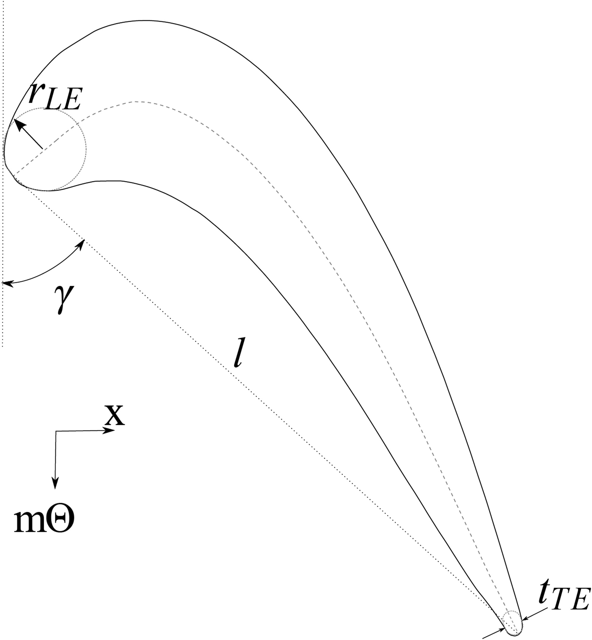
Table 1.
Digitised blade parameters as in the example in Figure 4.
Reconstruction of HPT blade and sample generation
The blade reconstruction is performed using an original CAD blade geometry and altered based on the difference between reference and measured blades. This difference is applied for all blade sections along the span. In this work, the reference blade is defined as the least deteriorated one. Changing the geometry of the leading- and trailing edge requires smoothing between the new circles (for leading-edge) or ellipses (for trailing-edge) and the rest of the profile geometry for obtaining a continuous surface. Otherwise, the algorithm used is based on Ernst et al. (2016).
The ranges of the parameters are shown in Table 1 and a total of 250 blades with different geometries is reconstructed, each representing a combination of different geometry parameters and surface roughness. In order to carry out the numerical experiment effectively, a uniform Latin-hypercube sampling (McKay et al., 2000) is used. The tip gap variations are included during the meshing process. The roughness is implemented in the CFD setup on both, the suction and the pressure side. The digitised blades of the first rotor stage belong to a V2500-A5, while only original blade geometries of all rows of the V2500-A1 are available for usage in the computational models. To overcome this issue, the geometric variations are normalised with the blade height, assuming that both variants of the V2500 show geometrically similar wear.
CFD simulations of HPT with deteriorated first rotor
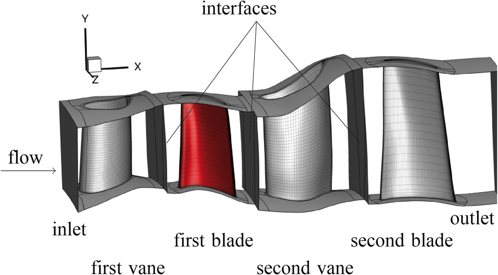
Based on the reconstructed blades, numerical set-ups are developed and simulated in a fully automated process. The CFD simulations are necessary to connect the effects of local deterioration, here first rotor blade, with the module performance. First, the meshes of the 2-stage HPT are constructed using
Although an accurate initial flow solution is used, a CFD simulation of a mesh with approximately 8 M cells requires about 84 CPUh for a converged solution. A mass flow difference between inlet and outlet, a change in efficiency, and a change in pressure ratio of less than 0.1% satisfy the stopping criterion.
For the validation the original CAD blade geometry with a hydraulically smooth surface is used. The CFD simulations predict a polytropic efficiency of 88.68%, a pressure ratio of 5.2, and a massflow of 47.28 kg/s, while performance simulation gives 88.80%, 5.1 and 48.02 kg/s for same boundary conditions. With the same setup a mesh convergence study is conducted, resulting in a GCI of 0.136% for the mass flow, 2.59% for the polytropic efficiency, and 0.005% for the pressure ratio.
Performance simulation of the overall aircraft engine
In order to evaluate the influence of isolated and combined module variances on the whole turbofan engine a performance model of the V2500-A1 aircraft engine is developed to analyse the on- and off-design performance. The model is part of a model-based non-linear gas path analysis (NLGPA) to calibrate the performance model to real aircraft engines (here a factory-new and deteriorated V2500-A1 turbofan engine (see Table 2)).
Table 2.
Maximum thrust 109 kN.
| Value | ||||||
|---|---|---|---|---|---|---|
| Unit | g/(kN·s) | kPa | K | K | rpm | Rpm |
| V2500-A1 | 10.23 | 142 | 850 | 806 | 4,981 | 13,972 |
| IFAS - V2500 A1 | 10.56 | 138 | 835 | 850 | 4,959 | 13,757 |
This analysis investigates the ranges in which the miscellaneous compressors and turbines wear out in addition to the HPT. In conjunction with the CFD simulations of the HPT, the NLGPA and, thus, the virtual process allow a combination of the overall aircraft engine performance with the local effect of deterioration. This analysis is presented by the schematic flow chart illustrated in Figure 6 and is implemented in Matlab (Kurzke and Halliwell, 2018; Salomon et al., 2021).
Figure 6.
Global off-design calculation procedure for high-bypass turbofans. Used for non-linear GPA and to train the artificial intelligence.
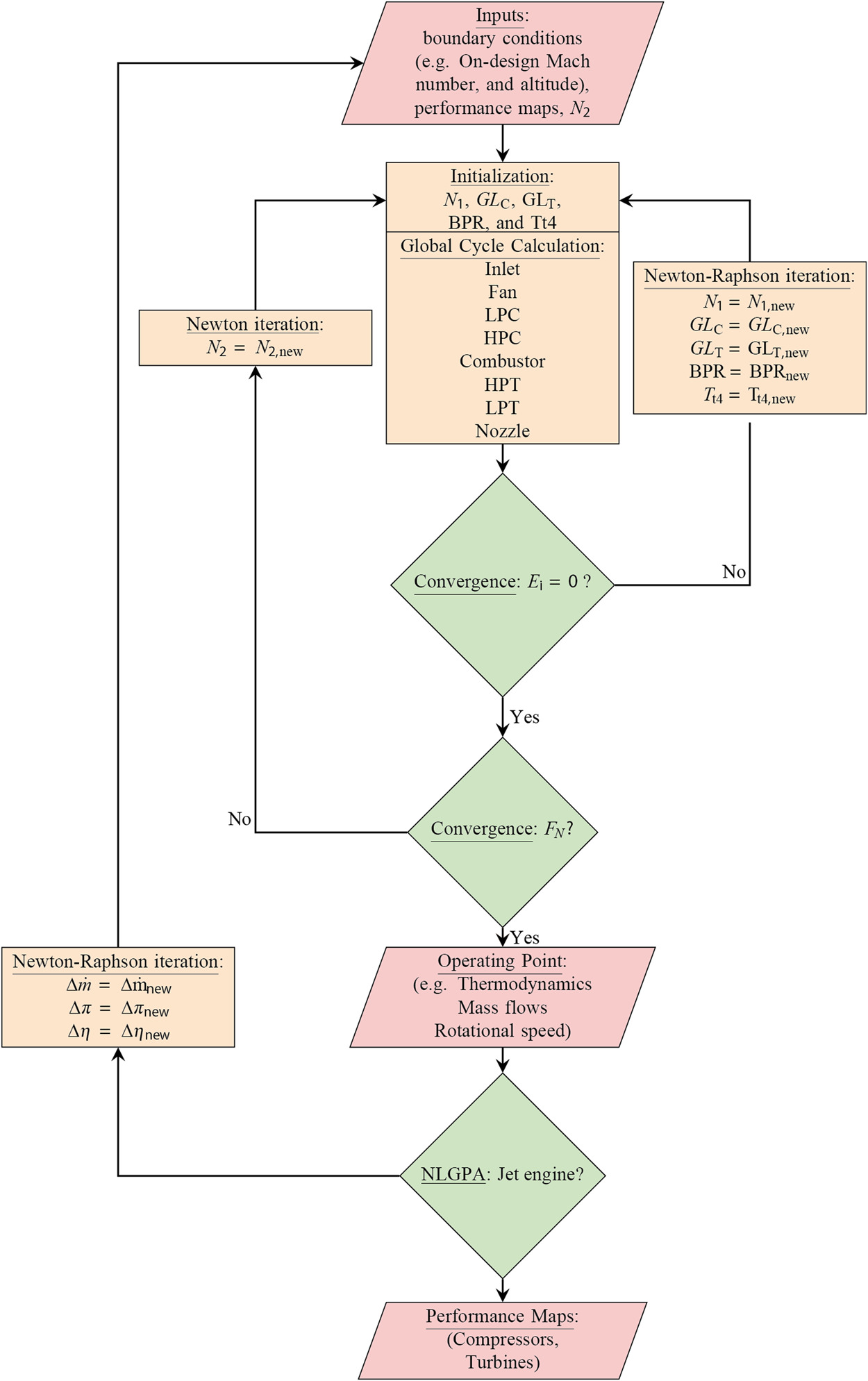
The off–design calculation procedure consists of an iterative simulation process which requires various input data, such as environmental conditions. Moreover, further aircraft engine-specific boundary conditions are required, being crucial for the thermodynamic cycle at a reference point, also referred to as the engine's on–design operating point. This point represents the basic framework of the jet engine and defines the interaction between the miscellaneous turbomachines, secondary air system, geometry (e.g. nozzle area), and number of revolutions in order to fulfil the thermodynamic cycle. Further boundary condition, such as the steady-state performance maps of the compressors and turbines are required. Hereon, quantities related to the compressor and turbines are denoted with
After the aircraft engine–specific boundary conditions have been imported and the operating point to be reached has been defined, the analysis starts the iterations. A distinction is made between the outer loop, in which the rotational speed
Based on the on–design input parameters, the initial values of all necessary parameters are provided for the first iteration. The iteration parameters for the inner loop at any rotational speed
The global aircraft engine matching process is described with these iterations and is used in the DoE to physically calculate the relationship between state of jet engine and performance output. The state of the engine is described by the variation of the maps through the scaling factors
In order to estimate the scaling factors for the LPC, IPC and HPC, as well as for the LPT, the performance model is calibrated to a factory-new and to the worn aircraft engine. The calibration is done via non-linear GPA, in which the performance map is iterated by scaling factors
Sensitivity analysis
A fundamental knowledge of the effects of variations in the input variables of a model on the output variables is of paramount importance in a variety of engineering domains. Sensitivity analysis examines precisely these relationships. Saltelli et al. (2004) provide the following definition of sensitivity analysis: ‘The study of how uncertainty in the output of a model (numerical or otherwise) can be apportioned to different sources of uncertainty in the model input’. Therefore, an effective and wide-ranged group of sophisticated sensitivity instruments are variance-based methods (Saltelli et al., 2010). The Sobol indices (Sobol, 2001) are a widely utilised representative of this type of sensitivity analysis tools for model outputs. These indices not only allow to identify the direct effects of particular input factors on the variances of output variables, but also of all potential impacts due to interaction effects between the variances of the inputs on the outputs.
Sobol indices
In the following text a brief description of the Sobol indices according to (Sobol, 2001; Saltelli et al., 2010; Kucherenko et al., 2012) is provided. For more information and a detailed derivation, see, e.g., (Sobol, 2001; Saltelli et al., 2010).
Consider a model
Normalising and decomposing Equation 8 by V leads to the closed-order effect index
Under the assumption of independent input variables, both Equations in 9 are known as Sobol indices. For the case of y being not arbitrary but univariate, i.e.
Kucherenko indices
Even though Sobol indices are an excellent tool for conducting comprehensive variance-based sensitivity analysis, their applicability is based on the constraining assumption of independent input variables. However, in practical applications, such as the interdependent performance of the miscellaneous modules inside of an aircraft engine, this assumption might be untrue. In Kucherenko et al. (2012) an approach is provided to generalise the Sobol indices that allows to perform comprehensive sensitivity analyses, taking into account dependencies among input variables.
The first-order effect Kucherenko index is formulated according to Equation 9 as:
and equivalent, the total-effect Kucherenko index is given by:withNote that the sum of all first-order effect Sobol indices is equal to or smaller than one, and the sum of all total-effect Sobol indices is equal to or greater than one (Glen and Isaacs, 2012). However, in the presence of dependencies in the model inputs, this does not hold for the Kucherenko indices. More information and a detailed derivation of the Kucherenko indices are provided in Kucherenko et al. (2012).
In practice, the analytical determination of the Kucherenko indices is often not feasible. Therefore, the present Monte Carlo estimators for their indices in Kucherenko et al. (2012), that are utilised in this work. Both estimators require a conditional sampling.
Metamodeling
In sensitivity analysis for the vast majority of cases, a relatively large sample size is mandatory. In aerodynamic engineering, however, many of the models employed are highly complex and simulations are consequently computationally demanding. As a result, generating sufficient samples is often too expensive or even unfeasible. A common approach to address this challenge is to develop and utilise metamodels that replicate the functionality of the original model, while being less complex and consequently less computationally intensive (see Shahsavani and Grimvall (2011) and Ben Abdessalem and El-Hami (2014)). In the context of aerodynamic engineering in general, and aircraft engine diagnostics in particular, such metamodels are increasingly based on artificial intelligence and deep learning approaches (see for example Khan and Yairi (2018) and Fentaye et al. (2019)). With these, larger sample sizes can be generated with less computational effort and thus, common sensitivity analysis tools can be applied.
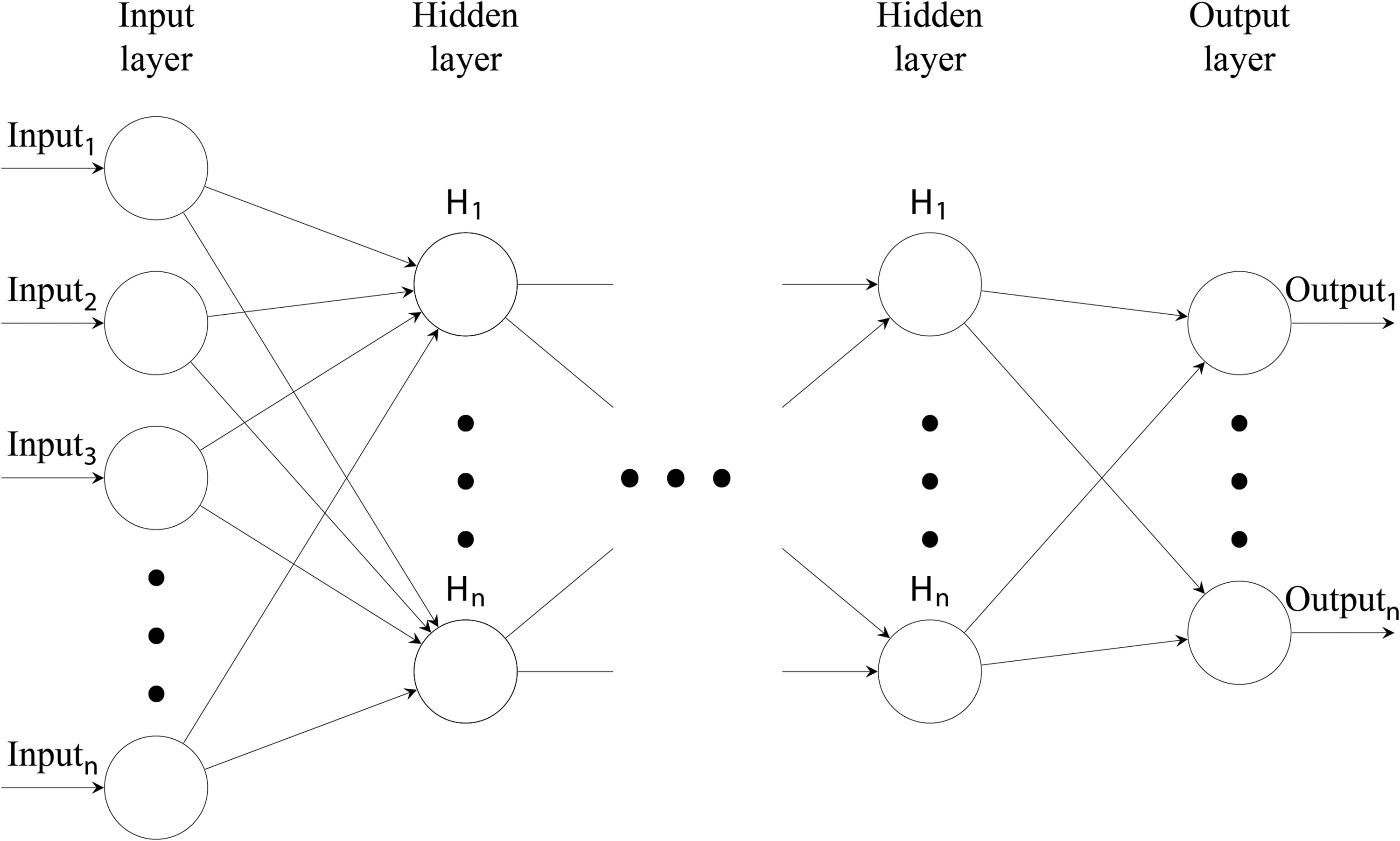
In this work, artificial neural networks are trained to guarantee a sufficient sample size for the respective sensitivity analysis. A schematic layout of such a network is shown in Figure 7. It basically consists of an input layer, one or more hidden layers and an output layer. The number of neurons per layer, as well as the number of hidden layers, depends on the particular original model and cannot be generalised. The number of input neurons, as well as the number of output neurons, typically follows the number of input and output variables of the model to be mapped. Each neuron of a layer is weighted connected to each neuron of the predecessor and successor layer. For a detailed description of neural networks in general and fitting function networks in particular, as well as their training and handling, see Rafiq et al. (2001) or Samarasinghe (2006). Note, that the utilization of an artificial neural network, such as employed in this work, represents only one potential approach among various approaches, such as, e.g., polynomial chaos expansion, to perform sensitivity analysis under the condition of a small data set. Here, the methods were exclusively chosen for the purpose to present proof of concept further methods will be investigated in subsequent work of the authors.
Results and discussion
The virtual process described in the methodology allows an instantaneous prediction of the effect of production scatter and of the deteriorated blades on the overall jet engine performance. Based on the physical model and metamodels the impact on aerodynamics and performance will be estimated.
HPT Sensitivities for single rotor deterioration
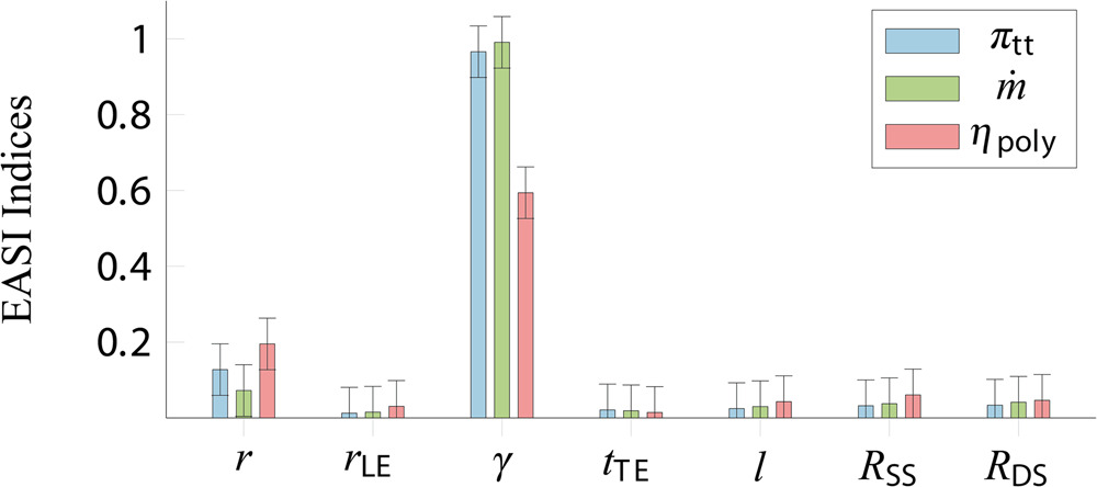
The performance sensitivity analysis of the overall aircraft engine requires significantly more than 211 performance samples of the HPT (see Figure 8). To expand the data, the described neural network as metamodel with three hidden layers, ten neurons per layer, eight input neurons, three output neurons, 15 epochs, and the Levenberg-Marquardt as back propagation algorithm is used. With these parameters a sufficient optimum was found, and for example, reducing the number of hidden layers results in a decrease in accuracy. Especially the epochs and neurons per layer showed an insensitivity for small changes in regards to prediction accuracy. For each neuron a sigmoid function is utilised as activation function. The final meta model reached a mean squared error of 1e-4 for all three outputs combined within a ten-times cross validation. Further improvement in accuracy would require more samples as well as further studies on different meta model approaches. The required extension of the geometric input is performed based on a Latin-hypercube sampling. Then, a variance-based sensitivity analysis is conducted on the input and output of the metamodel by means of Sobol indices (see Figure 9). This approach is validated by analysing the 211 original performance samples with the variance-based sensitivity approach according to Plischke (2010) and Plischke et al. (2013), so called EASI (Effective Algorithm for Computing Global Sensitivity Indices). This approach is purely based on existing data and does not require a specific input sampling. The sensitivity analysis is conducted on the three integral aerodynamic outputs in respect to the geometric inputs. First, a non-monotonic relationship is identified between mass flow and polytropic efficiency based on scatter plots. Classic correlation coefficients, e.g. Spearman's or Pearson's Rank correlation coefficient, are not sufficient in these cases. However, variance-based sensitivity studies are more suitable for detecting such non-monotonic relationships Saltelli et al. (2010). For the original CFD data the EASI indices of first-order indicate a direct sensitivity between stagger angle
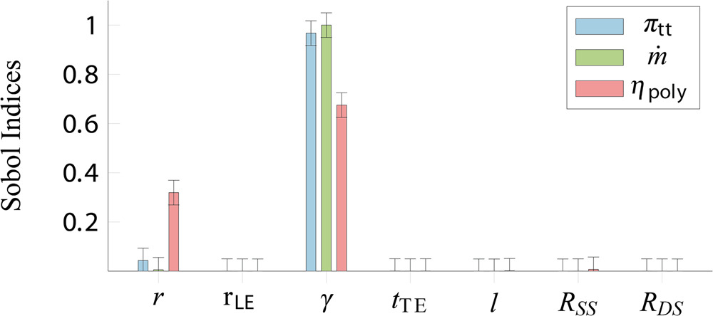
The sample size is increased according to Saltelli et al. (2004) with
It is shown that the estimated variance-based sensitivity analysis of the original data is similar to the Sobol analysis with a metamodel based on the original data. However, for this study it is only possible to analyse the direct relationship between inputs and outputs, i.e., first-order indices. Higher-order effects, that can show the systems interactions of input variables and their combined influence on the output variables, require larger sample sizes. Subsequently, an analysis of total-order effects purely based on the metamodel can not be validated and is therefore not conducted within this study.
Performance analysis
In order to estimate the impact on the overall performance of the V2500-A1 aircraft engine, the ranges of the scaling factors of each turbomachine have to be estimated. These ranges are determined on the one hand by CFD of the HPT, and on the other hand by the NLGPA of a factory-new and operational stressed aircraft engine V2500 (see Figure 6 and Table 2). The resulting scaling factors are an identifier for the real range of degradation of the compressors and turbines in the turbofan. These parameters are validated by previous studies (Goeing et al., 2020a) and further literature (Maiwada et al., 2016; Cruz-Manzo et al., 2018) (see Table 3). Thus, the
Table 3.
Scaling factors based on CFD, NLGPA and Literature.
| LPC | IPC | HPC | HPT | LPT | |
|---|---|---|---|---|---|
| 0.96 | 0.96 | 0.92 | 1.05 | 0.98 | |
| 0.96 | 0.96 | 0.92 | 0.95 | 0.98 | |
| 0.97 | 0.97 | 0.96 | 0.94 | 0.99 |
This metamodel is used with 1e6 random parameter configurations within the parameter space to evaluate the isolated and combined sensitivities. The input variables are interdependent, due to the power balance and mass conservation (see Equations 5 and 6), so a variance-based sensitivity analysis according to Kucherenko which is able to analyse such interdependent input variables is performed.
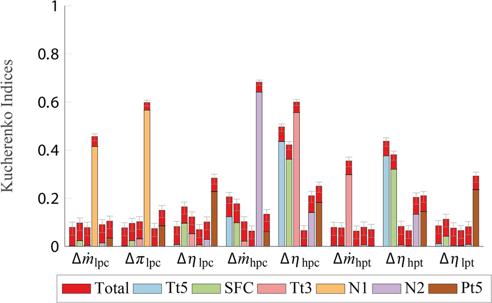
In Figure 10 the isolated (first) and isolated plus interacting (total) sensitivities of measurable variables are shown. Therefore, the first- order indices are represented with blue for Tt5, green (SFC), light red (Tt3), yellow (N1), purple (N2) and brown (Pt5) bars. The stacked red bars represent the total indices. Further on, the 95% confidence interval is shown as a black error bar for the first-order and a grey error bar for the total order. Scaling factors
As shown in Figure 10, most of the peaks are located at the HPC and HPT. In particular, the EGT (0.44/0.38) and the SFC (0.36/0.32) are responded to the efficiency of the HPC/HPT. It is noticeable that the temperature Tt3 reacts on the efficiency of the HPC (0.56), as well as the mass flow of HPT (0.30), while the mass flow of the HPC has a significant influence on the HP-System rotational speed N2 (0.64). N2 also reacts to the efficiency of the HPC/HPT (0.14/0.13). Furthermore, there is a significant relationship between N1 speed and the pressure ratio and the mass flow rate of the LPC (0.57/0.42). In addition, the pressure Pt5 reacts sensitively to efficiency of the LPC and LPT (0.23/0.24).
In order to illustrate the virtual process and to demonstrate the significance of the interactions on the overall performance, the described methods are performed with the real HPT blade in Figure 4 as an example. The geometry of the worn blade, roughness parameters, and of their confidence limits are derived and supplied to the process. Subsequently, the metamodel of the CFD is used to obtain the module aerodynamics and scaling factors. The HPT efficiency is reduced by 2.4 ± 0.2%, the pressure ratio is reduced by 0.046 ± 0.003, and the mass flow is increased by 0.64 ± 0.08 kg/s compared to new blades. These substantial aerodynamic changes of the scrapped HPT blade confirm the heavy deterioration stated earlier.
In the next step, these results are integrated in five aircraft engine configurations
Figure 11.
Impact on Tt5 of miscellaneous aircraft engine health conditions Θ
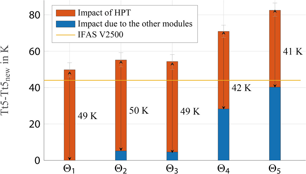
For this purpose, the Tt5 difference between the real and the new turbine blade over the various configurations
Conclusions
Variability in the modules due to production tolerances and wear directly affect the aircraft engine performance. To analyse this influence, a virtual process is developed which is able to predict overall aircraft engine performance, using the example of the first blade of the HPT in the V2500 turbofan engine. For this purpose, 36 deteriorated HPT blades are automatically digitised, their geometry evaluated, and their aero-thermodynamic effects determined at the level of the module. In a Gas Path Analysis of the HPT and the remaining modules (compressors and LPT), the overall aircraft engine performance is estimated. The use of CFD simulations for the HPT allows the local deterioration to be directly related to the engine performance, whereby a detailed understanding is established.
Based on the results of the physical models, metamodels are developed which are used to evaluate the isolated sensitivities within the HPT and isolated and interacting sensitivities within the aircraft engine. The results of variance-based sensitivity analysis can be summarised as:
Stagger angle
Next to
Tt5 and SFC react most strongly to
The sensitivity of a module with geometric variances on the aircraft engine performance depends on the condition of the remaining modules (see Figure 11).
The virtual process described shows that virtual twins are capable of evaluating aircraft engine performance. It is possible to integrate such a performance assessment with the virtual twin of an MRO shop as a basis for a rule-based decision making on component regeneration. The virtual twin even shows the possibility of matching certain deteriorated modules with each other and how this will impact the overall aircraft engine.
In future studies, the HPT process shown can be directly applied for further module evaluations (e.g. HPC, LPC, and LPT) that can be implemented in the aircraft engine performance analysis to characterise additional local deterioration effects. Furthermore, the described simplifications can be addressed and eliminated by larger sample sizes for further increasing the process accuracy. Finally, it is possible to further increase the accuracy of the process using more samples to compensate for the simplifications described.
Nomenclature
Mass Flow
η
Efficiency
γ
Stagger Angle
ω
Specific Dissipation Rate
π
Pressure Ratio
Θ
Jet Engine Configuration
AI
Artificial Intelligence
BPR
Bypass Ratio
C
Compressor
CAD
Computer-Aided Design
CFD
Computational Fluid Dynamics
DoE
Design of Experiment
EP, EP, EN
Error Function
EASI
Effective Algorithm for Computing Global Sensitivity Indices
EGT, Tt5
Exhaust Gas Temperature
f
Model Function
FN
Thrust
GL
Auxiliary Coordinates
H
Hidden Layer
h
Enthalpy
hp
High-Pressure
HPC
High-pressure Compressor
HPT
High-pressure Turbine
IAE
International Aero Engines
IPC
Intermediate-pressure Compressor (Booster)
k
Turbulent Kinetic Energy
ks
Equivalent Sand-Grain Roughness
l
Airfoil Chord
lp
Low-Pressure
LPC
Low-pressure Compressor (Fan)
LPT
Low-pressure Turbine
MRO
Maintenance, Repair and Overhaul
N1
Rotational Speed of LP-System
N2
Rotational Speed of HP-System
NLGPA
Non-linear Gas Path Analyse
p(·)
Distribution Function
p(·, · | ·)
Conditional Probability Density Function
p(·, ·)
Non-Conditional Probability Density Function
P
Pressure or Power
r
Tip Gap
rLE
Leading Edge Radius
RSS, RPS
Roughness Suction/Pressure Side
Sa
Surface Parameter
Sy
First-Order Effect Kucherenko/Sobol Index
Total-Order Effect Kucherenko/Sobol Index
SF
Scaling Factor
SFC
Specific Fuel Composition
T
Turbine or Temperature
t
Total
tTE
Trailing Edge Thickness
V
Variance
xi
Real-Valued Random Input Variable
Y
Model
y+
Non-dimensional Wall Distance