Large-Eddy Simulations of Rim Seal Flow in a One-Stage Axial Turbine

Thomas Hösgen; Matthias Meinke; Wolfgang Schröder

doi:10.33737/jgpps/129704

Introduction

The thermal efficiency of gas turbines strongly depends on the turbine inlet temperature. Increasing the inlet gas temperature for an improved engine performance results in several new challenges regarding the cooling of the machine. For instance, entering of hot gas from the main annulus flow into the wheel space between the stator and the rotor disks would lead to overheating and a significant reduction of the turbine lifetime. To avoid a hot gas ingress, cooling air from the turbine’s secondary air system is introduced into the wheel space, on the one hand, to cool the wheel space and on the other hand, to seal the rim seal gap at the stator hub. The primary goal is to minimize this cooling gas flow since the amount of secondary air directly deteriorates the turbine efficiency. Additionally, the mixing of the exiting cold gas with the main flow and its interaction with secondary flow structures, such as the vane hub passage vortex, causes further aerodynamic losses. The later has, for example, been investigated by Schuepbach et al. (2010) and Schädler et al. (2016).

Due to the large impact on the engine performance, the rim seal flow has been extensively studied over the past 50 years. A recent review of the progress made is given by Chew et al. (2019). Early studies of rim seal ingestion focused on the steady flow field inside the rotor-stator wheel space and the turbine hub region near the rotor-stator cavity. Two main driving factors of hot gas ingestion were determined (Johnson et al., 1994). The first effect is termed rotationally-induced ingress and can even occur without blading. Inside the wheel space the cooling air is radially pumped outward in the rotor disk boundary layer. This is also commonly called disk pumping effect. Further, the acceleration of the fluid by the rotor leads to a radial pressure gradient inside the wheel space. If the pressure falls below the pressure inside main flow passage, the hot gas enters the wheel space cavity. The second effect is termed externally-induced ingress and caused by non-axisymmetric pressure variations inside the main flow passage due to interactions of the stator vanes and the potential effect of the rotor blades. When the pressure in the hub region is higher or lower than inside the wheel space ingress or egress occurs.

Later studies focused on unsteady flow phenomena inside the rim seal cavity (Bohn et al., 2003; Rudzinski, 2009) were among the first to report unsteady pressure fluctuations inside the rim seal of a 1.5-stage turbine test rig. The unsteady flow structures were unrelated to blade passing and had significant impact on the sealing effectiveness. These unsteady phenomena were only present at low cooling gas mass flow rates and vanished abruptly when the cooling gas mass flux was sufficiently increased. The fluctuations were later confirmed by Jakoby et al. (2004), who conducted numerical simulations based on the unsteady Reynolds-Averaged Navier-Stokes (RANS)- approach of the same 1.5-stage turbine test rig. They compared solutions of several sector models with a full 360° simulation. Only the 360° simulation predicted a rotating mode inside the wheel space moving at about 80% of the rotor speed, and which had massive influence on the hot gas ingestion. They concluded that full 360° simulations are necessary to predict the hot gas ingress, since a sector model prohibits periodicities with an extent larger than the sector size. Similar findings were made by Cao et al. (2004). Unsteady RANS simulations unveiled periodic structures inside the rim seal, which were also observed in experimental studies. Complementing the conclusion of (Jakoby et al., 2004) the number of lobes of the periodic structures depended on the size of the chosen sector model.

The importance of these unsteady phenomena was later confirmed by Laskowski et al. (2009). The comparison of unsteady RANS simulations of a turbine model with simplified rotor blading showed significantly better agreement with experimental data than steady-state simulations. Although rotor rotation was neglected, Kelvin-Helmholtz type fluctuations were predicted inside the rim seal gap by the unsteady simulation. Such fluctuations were also found by Rabs et al. (2009) in their investigation of a sector model of a 1.5-stage axial turbine without blading. Adding blades, theses instabilities were still present, however, strongly reduced. Further studies showed that the unsteady flow phenomena strongly depended on the rim seal geometry (Chilla et al., 2013), and on the amount of injected cooling gas and the rotor speed (Beard et al., 2016).

O’Mahoney et al. (2010) performed a large-eddy simulation (LES) of a small sector model of a rim seal geometry with main annulus flow and compared it to unsteady RANS and experimental results. Significant discrepancies between LES and experiment were observed and the LES showed better agreement than the unsteady RANS solution. They concluded that increasing the LES grid resolution and increasing the size of the sector will lead to better solutions.

This study intends to increase the understanding of the inherent unsteady nature of the rim seal flow in axial flow turbines and follows the work of (Pogorelov et al., 2019). They conducted high fidelity LES of an axial flow turbine for the full 360° circumference of the main flow and the wheel space such that the uncertainty of RANS turbulence modelling and the limitations of a sector model was avoided. Two rim seal geometries were considered. They found Kelvin-Helmholtz type fluctuation inside a single lip axial rim seal gap, which interacted with the main annulus flow. Adding a second sealing lip supressed these fluctuations and reduced the hot gas ingress. In this paper, new results for the double lip rim seal geometry investigated by Pogorelov et al. (2019) are presented for a cooling gas mass flow rate reduced by 50%.

The paper is organized as follows. First, the governing equations and the numerical approach are discussed. Second, the computational setup, the investigated operating conditions, and boundary conditions are presented. Afterwards, the results of the flow field inside the rotor-stator wheel space are presented and compared to the results for the higher cooling gas mass flow rate from (Pogorelov et al., 2019). Finally, some conclusions are drawn.

Methodology

Governing equations

The motion of a viscous, compressible fluid is described by the Navier-Stokes equations. For an arbitrary moving control volume V with surface A, the conservation equations for mass, momentum, and energy read

(1)

ddt=∫V(t)QdV+∮A(t)H¯⋅ndA=0.

Here, Q=[ρ,ρu,ρE,ρY] is the vector of the conservative variables with the density ρ, the velocity vector ρu, the total energy ρE=ρe+ρu2/2, and the concentration of a passive scalar Y. The variable e denotes the specific internal energy. The quantity H¯ is the flux tensor and n the outward normal vector on the surface A. The flux tensor is split into an inviscid part

(2)

H¯inv=ρ(u−u∂V)ρu(u−u∂V)+pI¯ρE(u−u∂V)+ρuρY(u−u∂V),

and a viscous contribution

(3)

H¯vis=1Re00τ¯τ¯u+q−ρD∇Y/Sc0,

where (u−u∂V) is the velocity of the control volume’s surface, p is the pressure, and the unit tensor is given by I¯. Additionally, D is the mass diffusion coefficient of the passive scalar Y, and Sc0=1 is the Schmidt number. All variables are given in their non-dimensional form with respect to the variables at the state of rest denoted by “0”. The Reynolds number and the speed of sound are expressed by

(4)

Re0=(ρ0a0lref)/η0,

and

(5)

a0=γp0/ρ0,

with the ratio of specific heats γ=1.4 and the characteristic length lref. For a Newtonian fluid with zero bulk viscosity, the stress tensor is written

(6)

τ¯=(2/3)η(∇⋅u)I¯−η(∇u+(∇u)T).

The dynamic viscosity is computed using Sutherland’s law (Sutherland, 1893)

(7)

η(T)=T3/21+ST+S,

where S=111K/T0. For constant Prandtl number Pr0=0.72 the non-dimensional vector of heat conduction according to Fourier’s law is

(8)

q=−ηRe0Pr0(γ−1)∇T.

The equations are closed by the ideal gas relation, which is written in non-dimensional form

(9)

γp=ρT.

At fixed and at moving boundaries the no-slip condition is imposed. All walls are considered adiabatic. The pressure at the solid boundaries is determined via a robin-type boundary condition derived from the momentum equation.

Numerical method

The numerical method is based on a finite-volume solver and a level-set solver, which are efficiently coupled since both solvers hold individual subsets of a shared hierarchical Cartesian mesh. The shared base grid is generated by a parallel grid generator developed by Lintermann et al. (2014). During the solver run, the mesh is adapted according to the movement of the blade surfaces. The individual subsets of the grid are adapted separately and can differ even in regions where the domains of the solvers overlap.

The conservation equations (1) are discretized by a cell-centered finite-volume method. Following the large-eddy simulation (LES) approach, the turbulent structures are divided into the resolved part, which contains the dominant, large-scale, and most energetic eddies, and the unresolved part, which is modelled by the sub-grid scale model. An implicit filter is applied, where the filter width is determined by the length of the grid cells. The sub-grid contribution is modelled by the monotone integrated LES (MILES) approach (Boris et al., 1992), in which the discretization error of the numerical scheme is used to dissipate the energy at the unresolved scales.

A low-dissipation variant of the advection upstream splitting method (AUSM) proposed by Meinke et al. (2002) is used to calculate the inviscid flux tensor H¯inv (2). The primitive variables at the cell surfaces are obtained by a second-order accurate MUSCL extrapolation. The cell-centered gradients are computed by a weighted least-square method described in (Schneiders et al., 2016). The viscous flux tensor H¯vis (3) is computed using a central-difference scheme. The gradients at the cell-surface centroids are computed with the recentering-approach proposed by Berger and Aftosmis (2012).

The time-integration is performed by an explicit second-order accurate 5-stage Runge-Kutta scheme (Schneiders et al., 2016). This Runge-Kutta scheme is optimized for the efficient computation of moving boundaries. The Runge-Kutta coefficients are chosen for maximum stability. The time step fulfills the Courant-Friedrichs-Lewy (CFL) condition

(10)

Δt=CFL⋅mini=1,2,3h|ui|+a,

where h is the length of the smallest cell, ui the velocity in the direction i and a the speed of sound.

A strictly conservative cut-cell method is used to accurately represent the surfaces of embedded bodies, which are prescribed by a zero level-set contour obtained from the level-set solver. To prevent arbitrarily small time steps, a flux redistribution method is applied in small cut-cells. A detailed description of the cut-cell method and the flux redistribution method is given in (Schneiders et al., 2016).

A level-set approach is applied to describe the movement of embedded bodies. The level-set is a signed-distance function that divides the domain into a solid Gs and fluid Gf part

(11)

Gf(t)={x|Φ(x,t)>0},Γ(t)={x|Φ(x,t)=0},Gs(t)={x|Φ(x,t)≤0}.

The surface of the body is given by the zero level-set contour Γ. To preserve the resolution of the initial level-set surface while moving the bodies, the kinematic motion level-set approach described by Pogorelov et al. (2018) is used. In this method, the level-set solution at each time step is interpolated from the initial level-set field at the zeroth time step, which is reconstructed from high resolution stereolithography (STL)-data. Thus, the error in the surface representation only depends on the interpolation error and remains constant over time. This renders the method superior regarding other level-set approaches, such as the use of level-set transport equations, where the accuracy of the geometry representation can deteriorate over time.

A more general description of the solver can be found in (Lintermann et al., 2020), where more details of the solver structure are described along with performance measures.

Computational setup

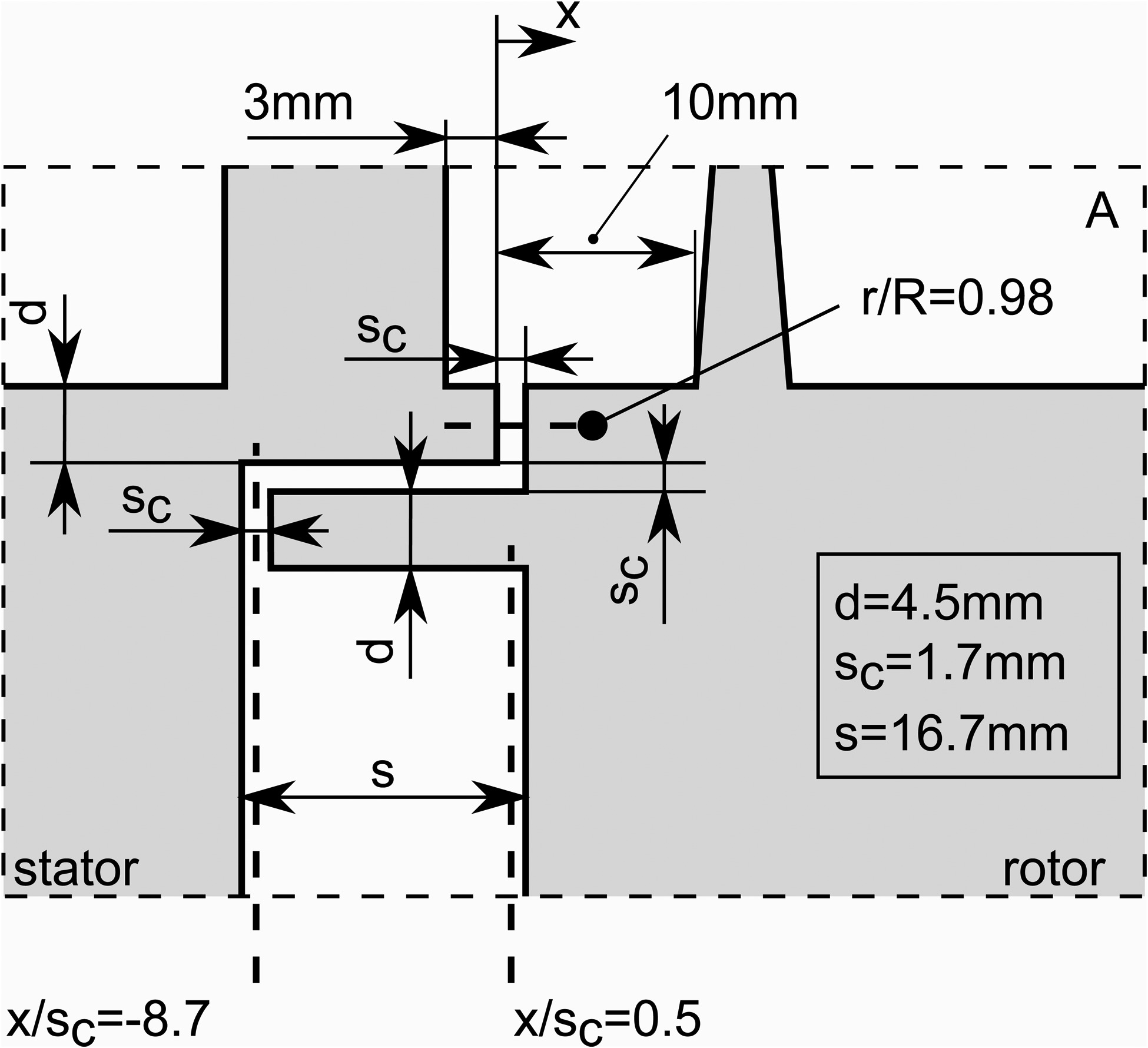
The one-stage axial flow turbine shown in Figure 1 is investigated. The stator and rotor are separately illustrated for the purpose of better visualisation. The turbine stage consists of 30 stator vanes and 62 rotor blades. A double lip rim seal is used to seal the rotor-stator wheel space. The upper seal lip is mounted on the stator and the second lip is mounted on the rotor disk. The turbine has been previously investigated by, for example, (Bohn and Wolff, 2003). Detailed experimental data is available in (Bohn and Wolff, 2001).

Figure 1.

Cut through the one-stage axial flow turbine; rotor and stator are separated.

https://journal.gpps.global/f/fulltexts/129704/JGPPS-00096-2020-01.01_min.jpg

The full 360° circumference of the main annulus flow and wheel space is resolved by an adaptive Cartesian mesh with approximately 450 million cells. The subset used by the finite-volume solver includes approximately 400 million leaf cells of the shared grid, while the level-set solver uses about 450 million leaf cells. Figure 2 shows an axial cut through the mesh. Two layers of refinement are used at the fixed and the moving boundaries. The size of the smallest regular, uncut cell is approximately 0.0017⋅R. A zoom of the rim seal geometry for the region marked in Figure 2 by the dashed line is displayed in Figure 3.

Figure 2.

Axial cut through the computational mesh.

https://journal.gpps.global/f/fulltexts/129704/JGPPS-00096-2020-01.02_min.jpg

Figure 3.

Schematic view of the rim seal geometry.

https://journal.gpps.global/f/fulltexts/129704/JGPPS-00096-2020-01.03_min.jpg

The operating conditions are defined by the four dimensionless quantities listed in Table 1. The subscript 1 indicates the flow state 1.5 mm downstream of the stator blades and cg denotes the conditions inside the cooling gas inlet. Two LES are conducted. Both LES share the same main flow operating condition (Rec1, Mc1) and rotor speed Reu. They differ in the dimensionless cooling gas mass flux cw, which is reduced by 50% in CW1K compared to CW2K.

Table 1.

Operating conditions.

	CW1K	CW2K
Rec1=ρ1c1Rμ1	0.8⋅106	0.8⋅106
Mc1=c1γRT1	0.37	0.37
Reu=ρcgΩR2μcg	0.8⋅106	0.8⋅106
cw=m˙cgμcgR	1,000	2,000

At the main and secondary inflow boundaries the density and the three velocity components are prescribed. Additionally, the velocity at the main inflow is superimposed by a synthetic turbulence with 5% turbulence intensity (Batten et al., 2004). At the outflow boundary, the static pressure is fixed. To reduce numerical wave reflections sponge layers are used at all in- and outflow boundaries. At the fixed and the moving walls, an adiabatic no-slip condition is prescribed.

Results and discussion

In the following, the numerical results of the flow field in the one-stage axial flow turbine for the two cases with different cooling gas mass flow rates are discussed. The operating conditions are listed in Table 1. The data for CW2K is taken from (Pogorelov et al., 2019). For both operating conditions, it takes approximately 40 full rotor rotations until the flow field is fully developed. This requires about 2,100 h of computing time on 4,800 cores on a CRAY XC40. A snapshot of the flow variables requires approximately 58.5 Gb of disc space. For the analysis only the final 3 rotations are considered. First, the mean flow fields in both LES are compared. Afterwards, the instantaneous flow field is analysed. Finally, the numerical results are compared against experimental data.

Figure 4 shows the azimuthal distribution of the time averaged effective radial velocity inside the rim seal gap at r/R = 0.98 (see Figure 3) for CW1K (−) and CW2K (…). The effective radial velocity is the radial velocity spatially averaged in the axial direction. In both LES the effective radial velocity evidences 30 distinct minima and maxima along the circumference, which are associated with the non-axisymmetric pressure distribution caused by the 30 stator blade wakes. The effective radial velocity becomes negative in the stator blade wake regions, which, therefore, is externally-induced ingress. In CW1K the averaged radial velocity is slightly lower due to reduced cooling gas mass flux. The root-mean-square (rms) values of the effective radial velocity fluctuation inside the rim seal gap are shown in Figure 5. The reduction of the cooling gas mass flux leads to reduced fluctuations in the rim seal gap.

Figure 4.

Azimuthal distribution of the time averaged effective radial velocity; CW1K (−), CW2K (…); r/R = 0.98.

https://journal.gpps.global/f/fulltexts/129704/JGPPS-00096-2020-01.04_min.jpg

Figure 5.

Azimuthal distribution of the effective radial velocity fluctuations; CW1K (−), CW2K (…); r/R = 0.98.

https://journal.gpps.global/f/fulltexts/129704/JGPPS-00096-2020-01.05_min.jpg

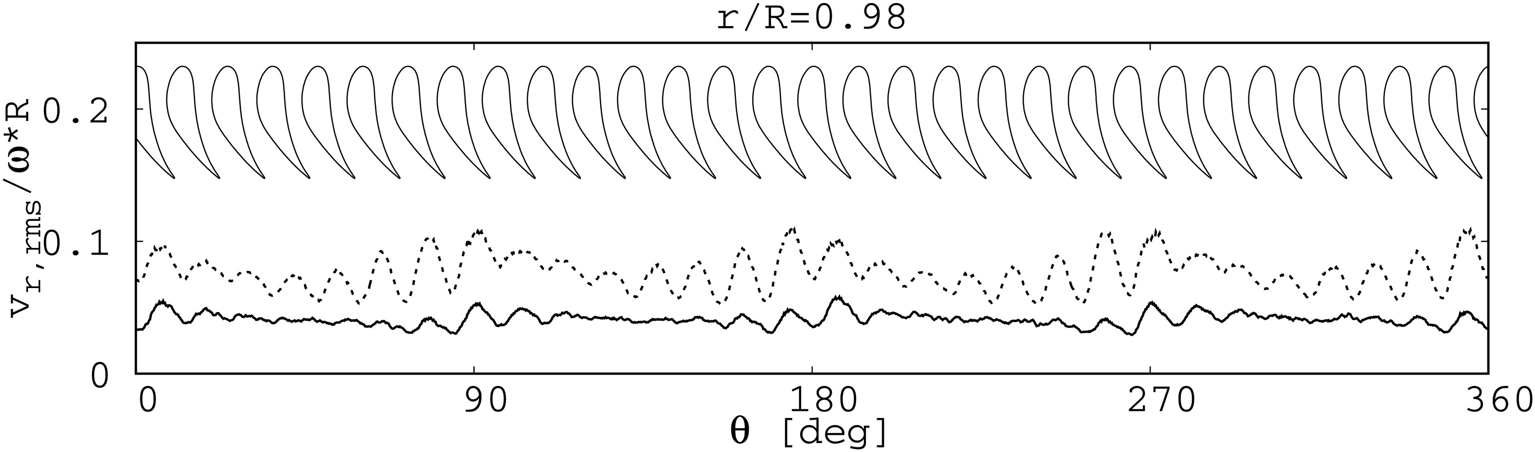
Figure 6 compares the radial distributions of the time averaged velocity components and pressure inside the wheel space at the fixed azimuthal position Θ=0∘. The distributions in two axial positions are investigated, i.e., near the stator wall at x/sc=−8.7 and near the rotor wall at x/sc=0.5 (see Figure 3). Due to the lower mass flux in CW1K (−), the cooling gas undergoes a stronger acceleration in the circumferential direction than in CW2K (…). The distributions of the radial velocities indicate the disk pumping effect, where the cooling gas is radially pumped outward near the rotor wall and flows radially inward in the stator boundary layer, which generates a large vortex structure in the time averaged flow field. The exact position of this vortex seems to depend on the cooling gas mass flux. The time averaged pressure level inside the wheel space is similar for both cooling gas mass fluxes. The pressure is normalized by the time and azimuthally averaged pressure inside the rim seal gap at r/R = 0.98. The deviation between both cases is less than 1%. Figure 7 shows the radial distributions of the rms values in the same axial and azimuthal positions. The rms values for the azimuthal velocity in CW1K (−) are lower than those in CW2K (…), while this behavior is reversed for the radial velocity. The pressure fluctuations show the strongest deviation. In CW2K, the pressure rms values are almost constant. In CW1K, they fluctuate significantly about a mean value which exceeds the rms values in CW2K by a factor two. To identify the reason for the increased pressure fluctuations, the instantaneous flow field inside the wheel space is investigated more thoroughly. The pressure signals inside the wheel space have been recorded over 3 full rotor rotations and sampled in 408 radially distributed bins along the stator wall. For these signals cross-correlations are computed relative to the signal at location r/R=0.98. The results are depicted in Figure 8. The square pattern for CW1K (left) indicates the existence of a standing wave inside the rotor-stator wheel space. For CW2K (right), no distinct pattern can be observed.

Figure 6.

Time averaged radial distributions of the velocity components and the pressure at two axial positions; CW1K (−), CW2K (…).

https://journal.gpps.global/f/fulltexts/129704/JGPPS-00096-2020-01.06_min.jpg

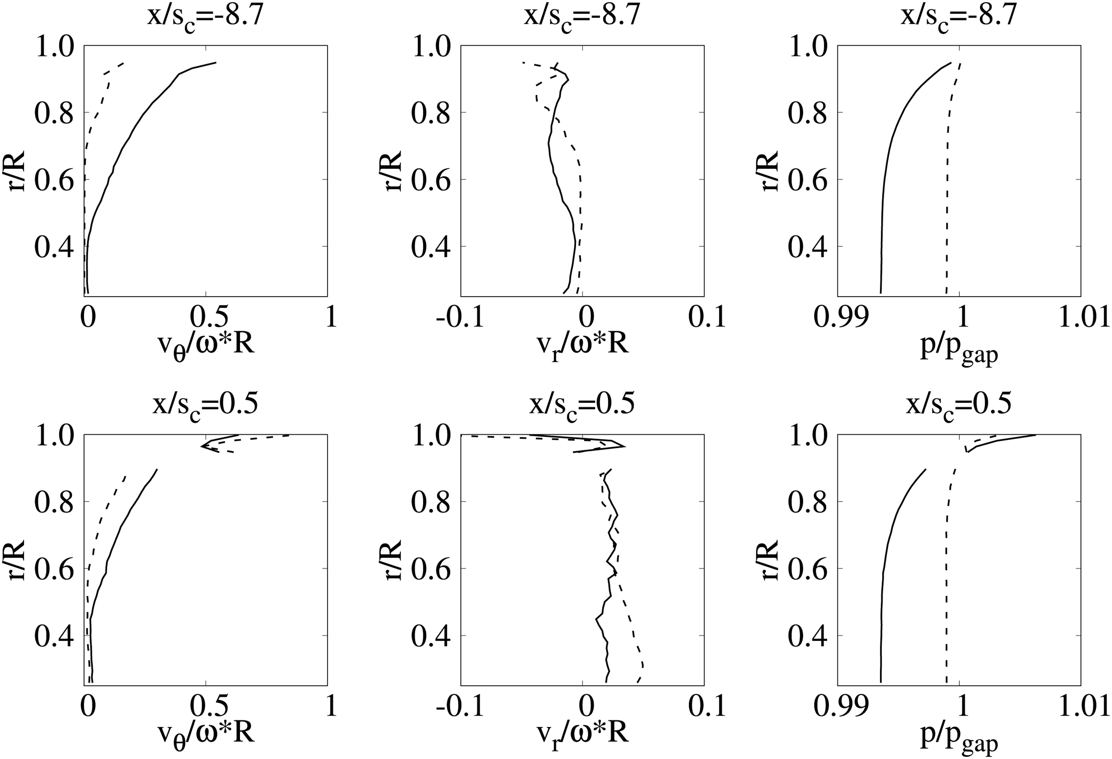
Figure 7.

Radial distributions of the velocity components and the pressure fluctuations at two axial positions; CW1K (−), CW2K (…).

https://journal.gpps.global/f/fulltexts/129704/JGPPS-00096-2020-01.07_min.jpg

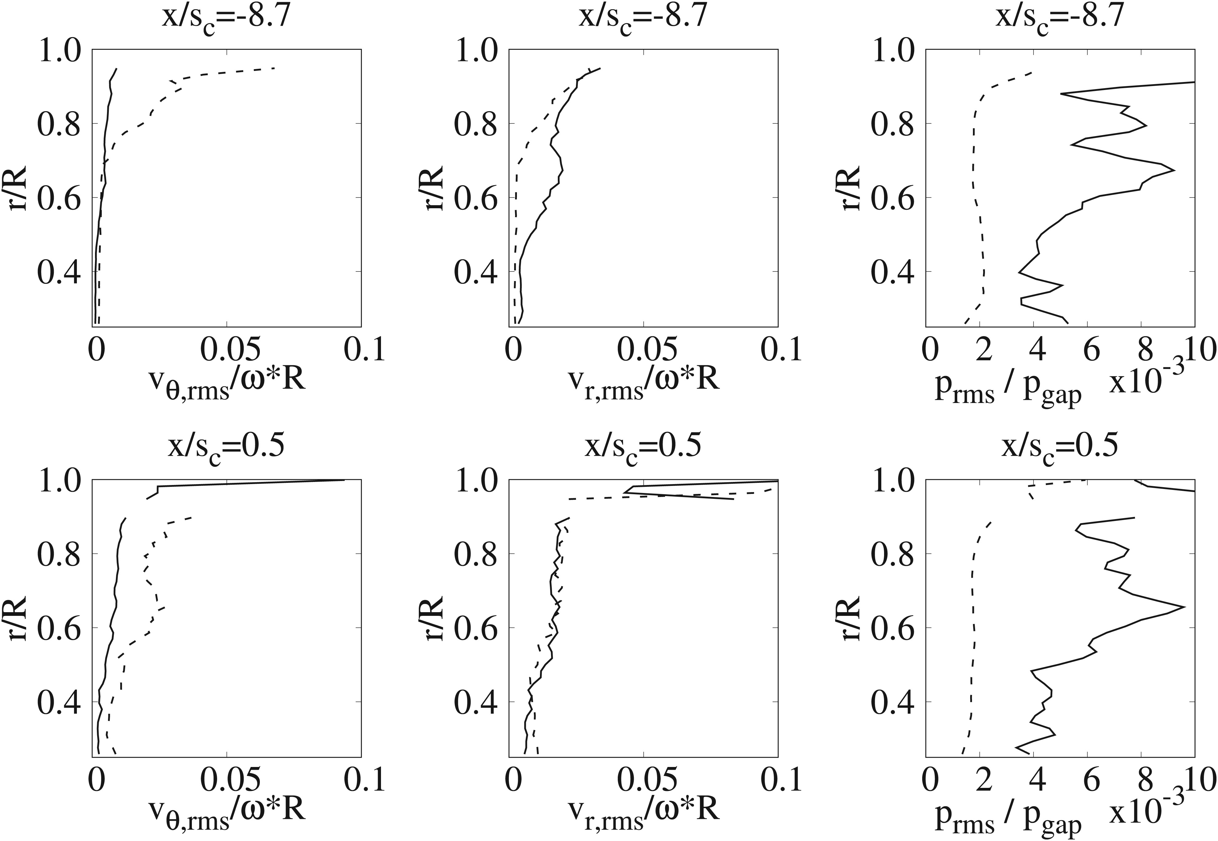
Figure 8.

Cross-correlations computed from the pressure fluctuations along the stator wall inside the wheel space; CW1K (left), CW2K (right).

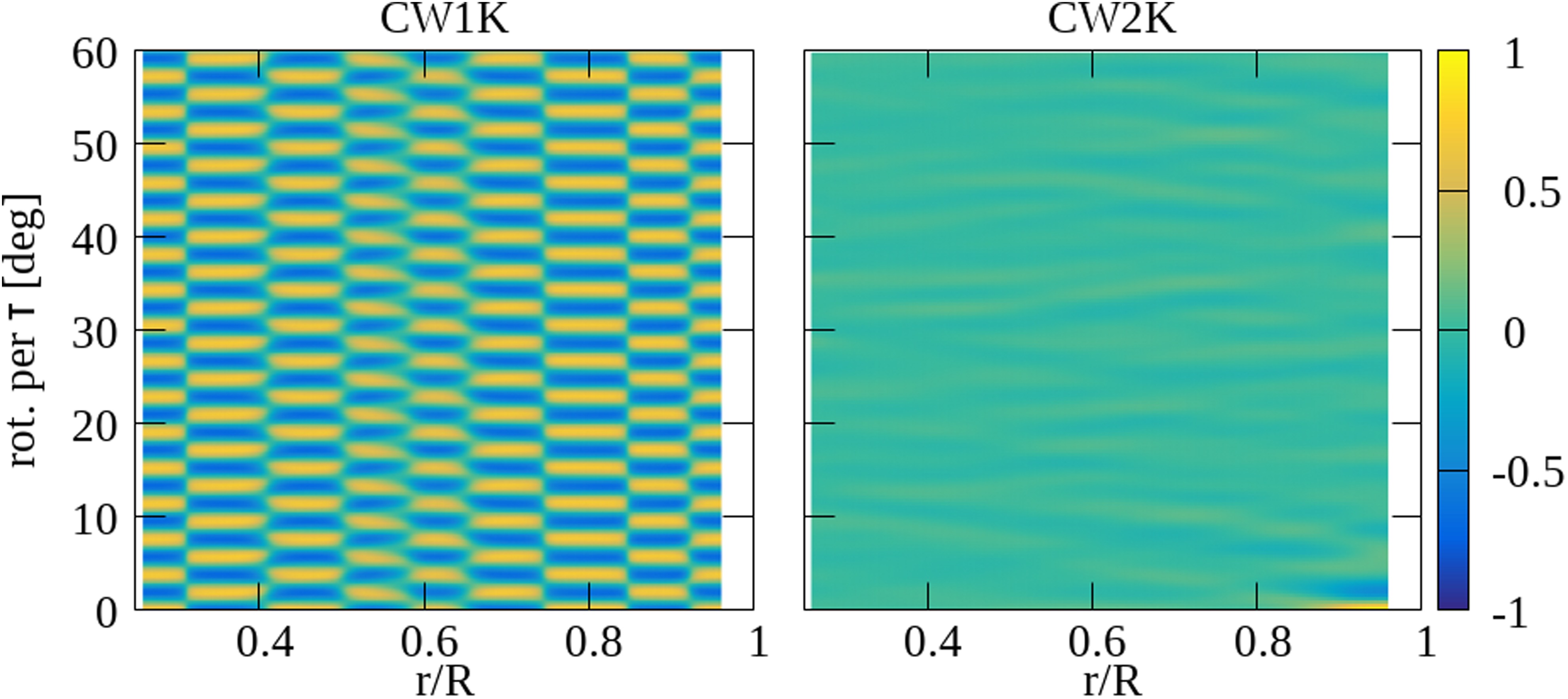
https://journal.gpps.global/f/fulltexts/129704/JGPPS-00096-2020-01.08_min.jpg

This is further confirmed when the energy spectra computed form these cross-correlations are investigated. Figure 9 shows that the energy spectrum for CW1K (top) features a distinct peak at a frequency of approximately 94.33 times the rotor speed n, which exists along the entire stator wall. For the sake of conciseness only the spectrum at the radial position r/R=0.6 is shown. The energy spectrum of CW2K (bottom) only shows a minor peak at the blade passage frequency (BPF) f/n=62. Note that the low local minima and maxima in the pressure rms values of CW1K in Figure 7 coincide with the nodes of the standing wave seen in the respective cross-correlation in Figure 8.

Figure 9.

Energy spectra computed from cross-correlations of the pressure fluctuations along the stator wall inside the wheel space; CW1K (top), CW2K (bottom); x/s_c = −8.7.

https://journal.gpps.global/f/fulltexts/129704/JGPPS-00096-2020-01.09_min.jpg

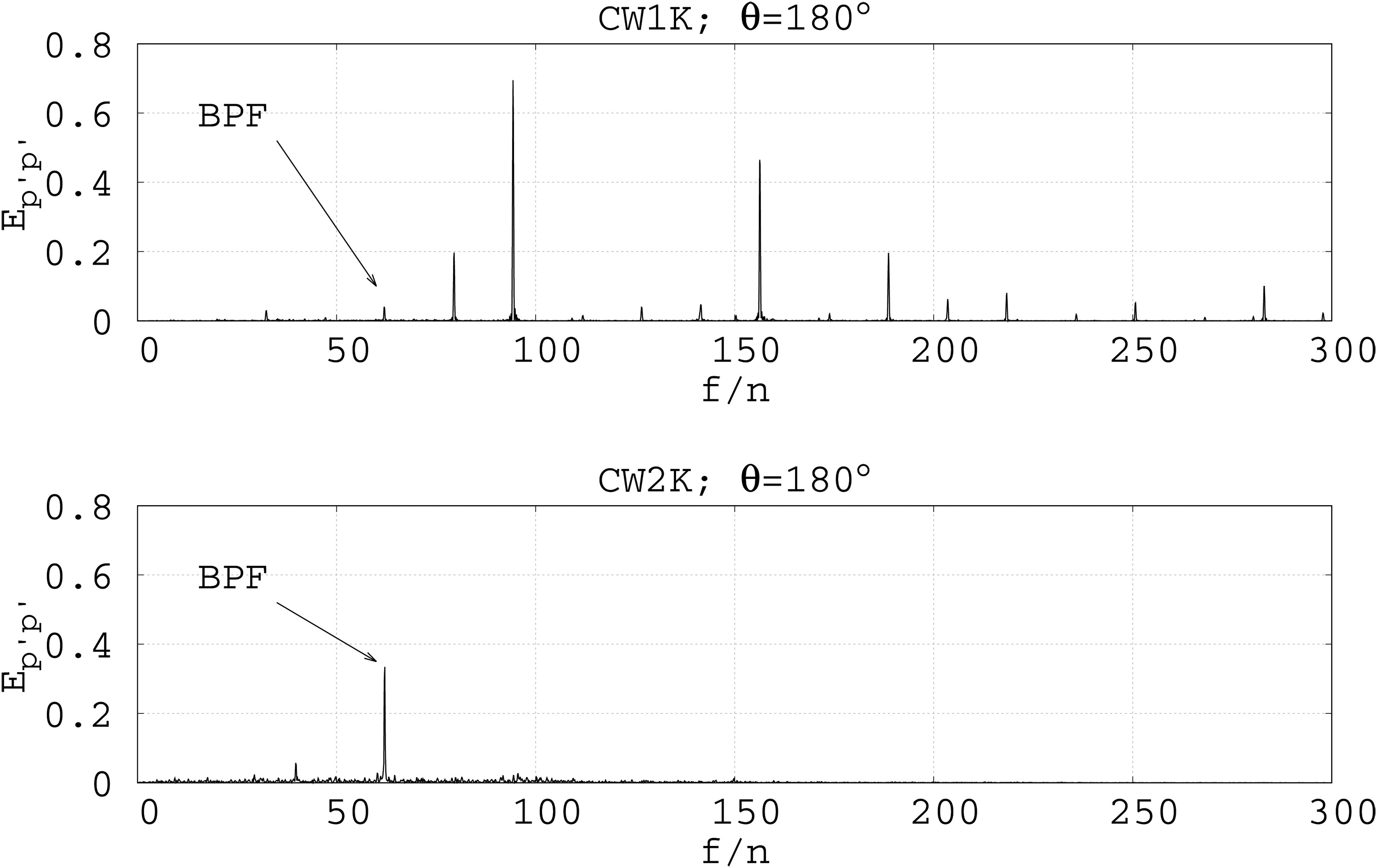
This dominant frequency in CW1K is also found in the instantaneous flow field inside the rim seal gap at r/R=0.98. The signals of the pressure and the effective radial velocity were recorded over 3 full rotor rotations along the entire circumference in 1,440 equidistantly spaced positions. Using the same procedure as described for the energy spectra in Figure 9, the energy spectra of the pressure fluctuations and the fluctuations of the effective radial velocity inside the rim seal gap are obtained. Due to the page limit the energy spectra are only shown for the position Θ=180∘. The pressure energy spectrum of CW2K (bottom) in Figure 10 only evidences the blade passage frequency at f/n=62. For CW1K (top), however, not only the blade passage frequency but a wide range of frequencies from f/n=30 to f/n=300 is apparent. The most dominant frequency is the one which has already been determined inside the wheel space at f/n≈94.33.

Figure 10.

Energy spectra computed from cross-correlations of the pressure fluctuations inside the rim seal gap; CW1K (top), CW2K (bottom); r/R = 0.98.

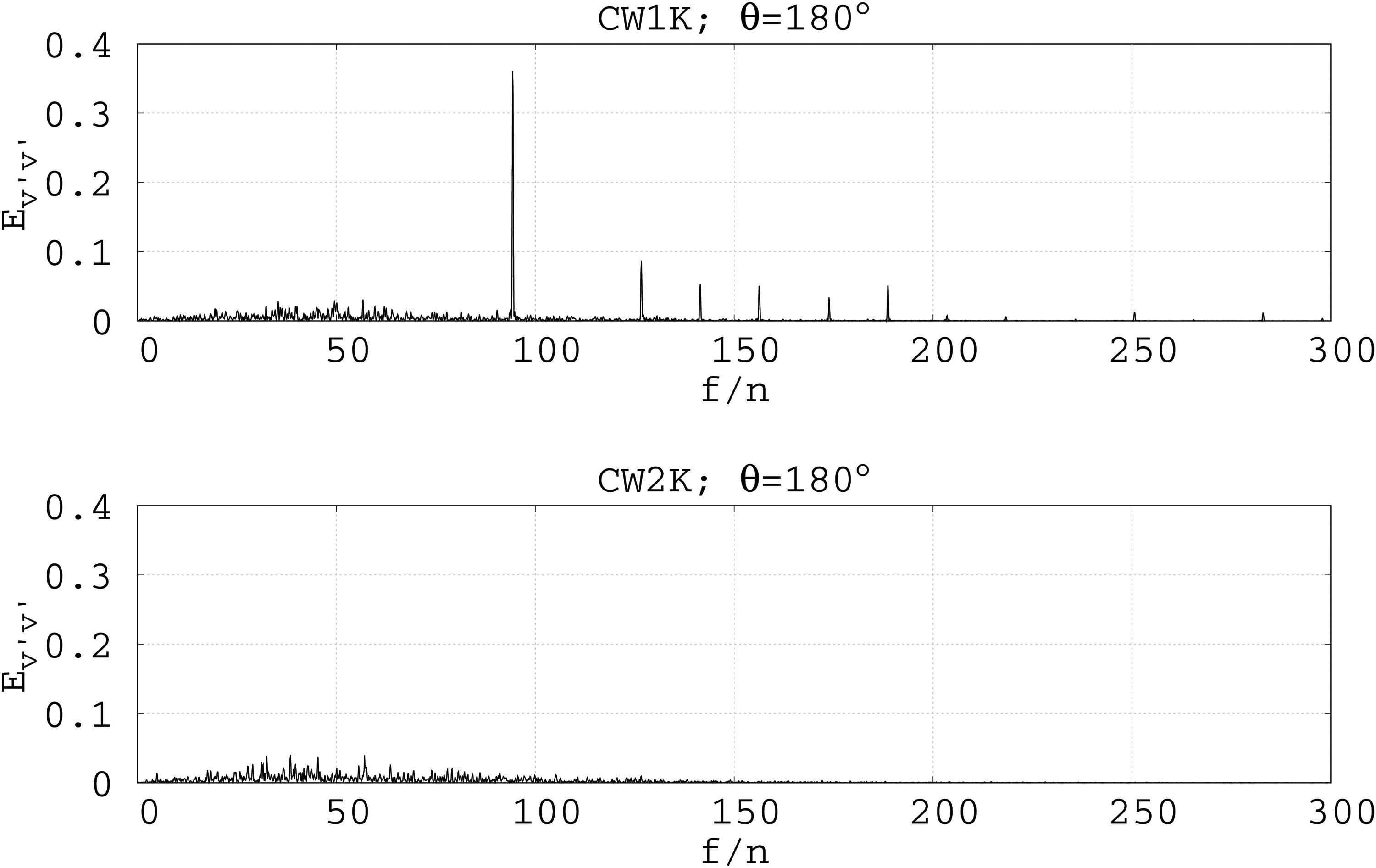
https://journal.gpps.global/f/fulltexts/129704/JGPPS-00096-2020-01.10_min.jpg

The energy spectrum of the effective radial velocity fluctuations for CW1K in Figure 11 (top) shows the same frequency as the pressure fluctuations for CW1K in Figure 10, however, with differently pronounced amplitudes. Below the dominant frequency f/n≈94.33 only a band of elevated frequencies is observed. This is also apparent for CW2K (bottom).

Figure 11.

Energy spectra computed from cross-correlations of the effective radial velocity fluctuations inside the rim seal gap; CW1K (top), CW2K (bottom); r/R = 0.98.

https://journal.gpps.global/f/fulltexts/129704/JGPPS-00096-2020-01.11_min.jpg

The acoustic eigenfrequencies of a closed pipe can be calculated by

(12)

f=m2⋅L⋅a,

with a the speed of sound, L the length of the resonator, and m the order of the harmonic. Inside the wheel space the Mach number is low and the speed of sound almost constant. For CW1K, the ratio of the speed of sound and the circumferential speed is approximately a/ωR=2.853. Using the height of the wheel space L=R−(2⋅d+sc)−rh=86.65mm the harmonics can be determined. The data are listed in Table 2.

Table 2.

Harmonics of a closed pipe normalized by rotor speed f/n.

m	7	8	11	12	13
Theory	84.17	96.20	132.27	144.29	156.32
LES	79.53	94.33	126.6	141.5	156.3
rel. Error	−5.5%	−1.9%	4.2%	−1.9%	−0.01%
m	16	17	18	21	24
Theory	192.39	204.42	216.44	252.51	288.59
LES	188.7	203.5	218.3	250.6	283.1
rel. Error	−1.9%	−0.5%	0.9%	−0.8%	−1.9%

Of course, to approximate the wheel space by a closed pipe is pretty crude, since the mean pressure increases radially, and the mean flow velocity is not zero. Nevertheless, the 8th harmonic lies very close to f/n≈94.33.

The comparison of the LES data for CW1K from Figure 10 with the theoretical finding shows a good match. The strongest deviations between the theoretical values and the LES occur for the frequencies being close to a multiple of the blade passage frequency, i.e.

(13)

fn=x⋅62.

Apparently, the rotor-stator interaction and the turbulent fluctuations inside the shear layer between the main flow and the exiting cooling gas excite several of the wheel spaces’ harmonics. This, in turn, results in the development of a standing wave inside the wheel space.

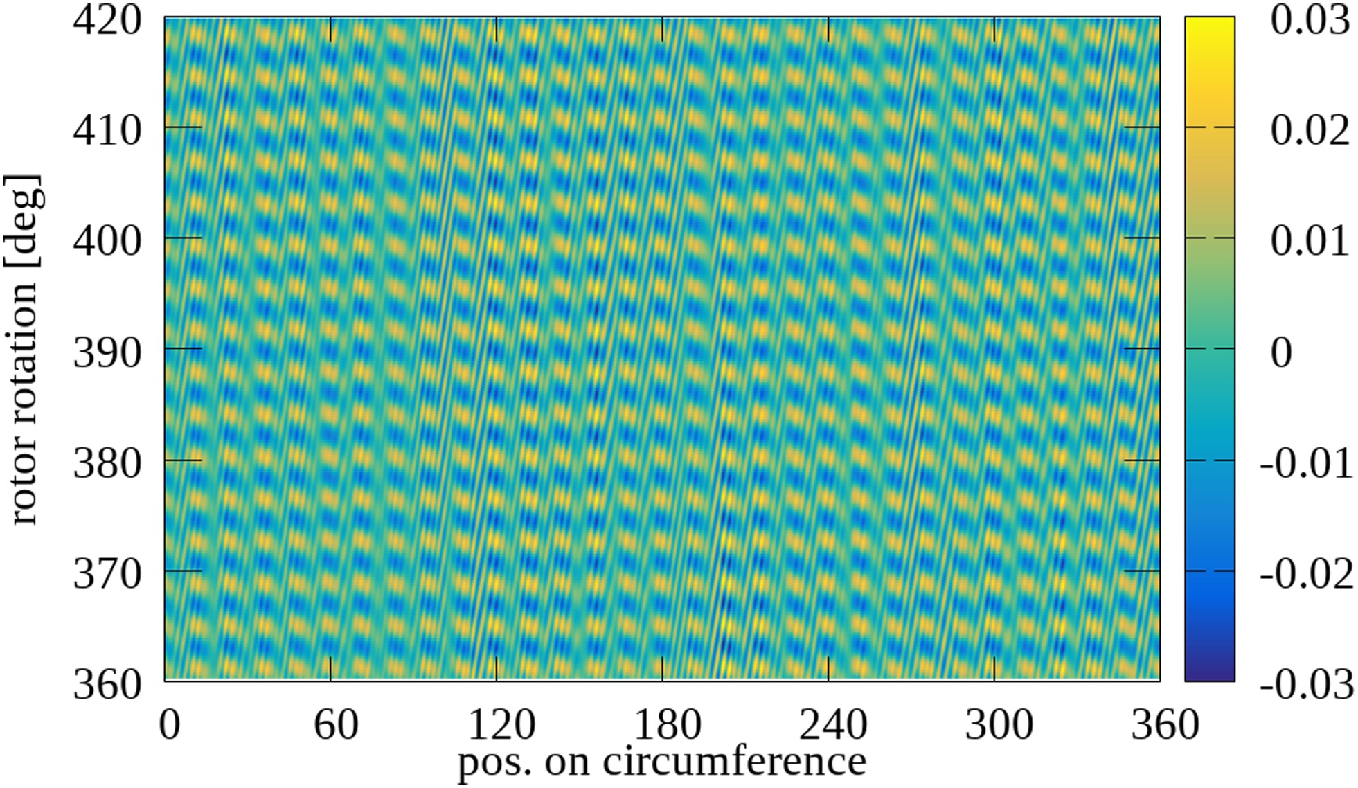
To analyze the impact of the dominant 8th harmonic at f/n=94.33 a fourth-order Butterworth bandpass filter is applied to the flow field of the effective radial velocity inside the rim seal gap. The result is shown in Figure 12 for a time period of 60∘ rotor rotation. A square pattern consisting of 30 fields in the azimuthal direction and a strong fluctuation in time is evident for the filtered effective radial velocity v~r. The 30 azimuthal fields correspond to the 30 stator blades. The temporal fluctuation repeats approximately every 3.82∘ rotor rotation and corresponds to the standing wave inside the wheel space. Interestingly, this temporal fluctuation leads to alternating positive and negative values of the effective radial velocity with an amplitude of the same order as the mean effective radial velocity inside the rim seal gap (Figure 4). Hence, the standing wave triggers alternating cold gas egress and hot gas ingress. Therefore, it has a major impact on the cooling effectiveness.

Figure 12.

Filtered effective radial velocity v~r/ωR inside the rim seal gap at r/R = 0.98; CW1K.

https://journal.gpps.global/f/fulltexts/129704/JGPPS-00096-2020-01.12_min.jpg

The impact of the 8th harmonic on the cooling effectiveness is displayed by the radial distribution of the time and circumferentially averaged cooling effectiveness for CW1K and CW2K in Figure 13.

Figure 13.

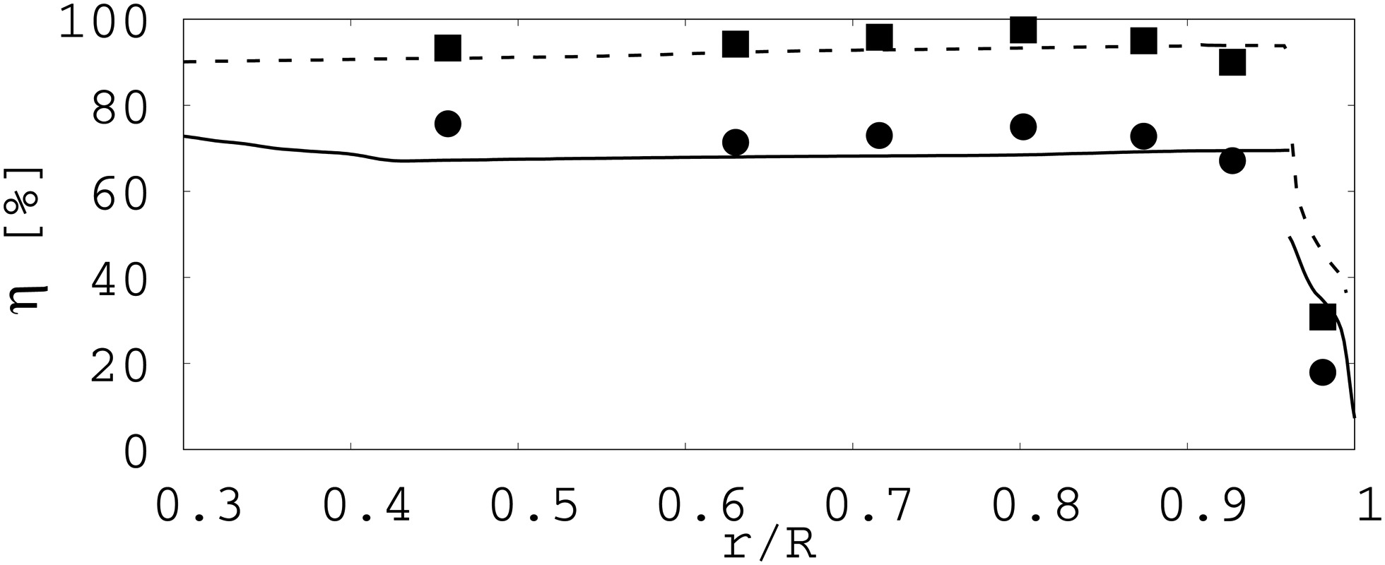
Radial distribution of the time and azimuthally averaged cooling effectiveness; LES: CW1K (−), CW2K (−−−), exp. data (Bohn and Wolff, 2001): CW1K (∙), CW2K (▪).

https://journal.gpps.global/f/fulltexts/129704/JGPPS-00096-2020-01.13_min.jpg

The cooling effectiveness is computed by

(14)

η=Y(r)−YhgYcg−Yhg,

where Y is the concentration of a tracer gas mixed into the cooling gas. The concentration is obtained from a passive scalar transport equation. The subscripts hg and cg denote the concentrations at the main flow and the cooling gas inlet. In both cases the LES results match the experimental data from (Bohn and Wolff, 2001) convincingly. For CW1K, the cooling effectiveness is significantly reduced compared to CW2K, since none of the wheel space’s harmonics are excited for CW2K.

Conclusions

The flow field for two cooling gas mass flow rates of a one-stage axial flow turbine has been investigated. Approximately 40 full rotor rotations were necessary to reach a statistically converged flow field.

It was shown that the reduction of the cooling gas mass flux has only little effect on the time averaged flow field inside the wheel space. The instantaneous flow field, however, is strongly influenced by the amount of cooling gas. For the lower cooling gas mass flux (CW1K), several of the wheel space’s harmonics are excited. This leads to the development of a standing wave inside the rotor-stator wheel space, which has a significant impact on the radial velocity inside the rim seal gap. Over one time period of that wave, cooling gas is blown out of the wheel space, followed by a suction of hot gas from the main annulus into the wheel space. For the higher cooling gas mass flux (CW2K), the wheel space’s harmonics are not excited.

The suction of hot gas into the wheel space in CW1K, caused by the excited 8th harmonic of the wheel space, results in a significantly reduced cooling effectiveness compared to CW2K. In brief, it can be concluded that there is a critical cooling gas mass flux above which the turbulent fluctuations inside the rotor-stator cavity are stabilized.