Introduction

The design of modern, efficient turbomachinery requires the consideration of secondary flow during early design stages (Cumpsty, 2010). In order to do so, the numerical tools used during the design are subject to continuous improvements. The design tools must account for unsteady flow phenomena in addition to steady-state or time-averaged secondary flow.

This paper presents and analyses unsteady flow phenomena measured in the cavity outlet of a turbine shroud labyrinth seal. Unsteady pressure fluctuations such as those reported in this paper have often been found in rim seal cavities. However, there are currently no studies the authors could find in open literature focussed on similar phenomena inside shroud cavities at turbine blade tips. The occurrence of the unsteady fluctuations, as evident in the pressure spectrum measured in the data at hand, may be explained satisfactorily by means of a simple kinematic theory presented in this paper.

In analysing the data, the following questions are addressed: (1) What is the cause of the unsteady pressure fluctuation in the labyrinth seal cavity outlet? (2) Which parameters influence the occurrence of the unsteady phenomenon? (3) Can the phenomenon be reproduced in CFD, i.e. modelled correctly?

There is previous research, both experimental and numerical, into unsteady flow phenomena in rim seal cavities in axial turbines. However, the similarity of unsteady flow phenomena observed in the rim cavities to those in tip shroud cavities reported in this paper is remarkable as shown in the results section below.

Beard et al. (2017) conducted an experiment on a rim seal test rig operated without mainstream air and without blades in the main channel. They identify a flow structure with 27 to 29 lobes in the rim seal rotating at an angular speed of ωs/Ω≈0.8, i.e. approximately 80% of the rotor speed. The study shows that increasing the rotational speed or the sealing mass flow reduces the number of lobes. The corresponding numerical studies were conducted by Gao et al. (2017). LES and URANS simulations in the latter study show reasonably good agreement with steady-state measurements within the disc cavity when compared with experimental data. Unsteadiness at a similar distinct peak frequency can only be found in the LES. The authors suspect the discrepancies in number of lobes, structure, and rotational velocity to be caused by the limited circumferential sector of the numerical model or other approximations.

Boudet et al. (2006) investigate the rim seal of an axial turbine by means of numerical simulations. The results show fluctuations at frequencies lower than the blade passing frequency. Further simulations show that the instability develops inside the seal cavity. The authors associate the phenomenon with Taylor-Couette instability, as the conditions for the flow regime are met inside the rim seal. There is no information concerning the rotational frequency of the fluctuations.

Numerical simulations with two set-ups are conducted by Rabs et al. (2009). In the first numerical simulation, the guide vanes and blades are omitted, resulting in a simplified turbine rim cavity model. The pressure distributions show regions with high and low pressure in circumferential direction due to Kelvin-Helmholtz vortices. In a second simulation, a full model of a 1½-stage turbine is modelled. Here, the vortices appear at high non-dimensional sealing air mass flow rates and are suppressed by the interaction of the guide vanes and the blades for low and medium flow rates. The magnitude and frequency of the occurrence is decreased compared to the simplified model.

Boutet-Blais et al. (2011) conducted numerical simulations of a simplified turbine rim seal environment without blade and vanes. Large-scale structures with 29 regions of high and low pressure inside the seal cavity were identified, which rotate at ωs/Ω≈0.79. The study notes that the frequency corresponding to this effect is far more energetic than that of the blade passage. Furthermore, it shows that the presence of these large-scale structures directly influences the seal effectiveness.

Cao et al. (2004) study the interaction of rim seal and annulus flows by means of numerical computations as well as experiments. They identify unsteady flow structures with 11–14 nodes inside the rim seal rotating at slightly less than rotor speed. The unsteadiness causes peaks in the spectrum in the range of 600–800 Hz. Further examination suggests that the number of nodes around the annulus varies over time.

Horwood et al. (2018) conducted a combined experimental and computational investigation. The study also identified structures, which rotate at an angular velocity of ωs/Ω=0.81…0.94 and ωs/Ω=0.92…1.03 in simulation and experiments, respectively. The study names Kelvin-Helmholtz instabilities as the cause. In a later publication, Horwood et al. (2020) examine further operating conditions. The peak-frequency and amplitude of the phenomena are found to be dependent on the sealing purge flow. The statement concerning the cause of the large-scale structure is amended to include Taylor-Couette instabilities.

Hualca et al. (2020) state that the positions of vanes and the presence of blades affect the rotating structures. The frequency of signal peaks is weakly dependent on the vane position and the sealing mass flow. Without the rotor blades, structures with 34 to 40 lobes that rotate with ωS/Ω=0.71…0.98 were identified. With rotor blades, the number of lobes is reduced to 22 to 28 and the structures rotate with ωS/Ω=0.96…1.12.

Numerical simulations by Jakoby et al. (2004) show three low pressure regions inside the cavity, which rotate with ωS/Ω=0.80. With an increase in the cooling air mass flow, the phenomenon disappears. Similar findings are presented by Julien et al. (2010). Large-scale structures with 30 lobes are detected for no and low purge flow conditions. The coherent structure in this study rotates at ωS/Ω=0.87 and 0.80, respectively. In the case of a high purge flow condition, only smaller pressure pulses deeper inside the cavity instead of large-scale structures can be found.

Schaedler et al. (2016) also detect low frequency pressure fluctuations in an experimental and numerical investigation. The structures are dependent on the purge mass flow as the band of frequencies with elevated amplitudes is shifted to higher frequencies when the purge mass flow is increased. It is not present for the highest injection rate. The number of lobes (8 and 22, respectively) and angular velocity (ωS/Ω=0.82 and 0.93, respectively) are derived from the numerical simulation. The pressure fluctuations have a significant impact on the noise level as an increase of up to 18 dB can be detected when the structures are present.

Using URANS-based CFD-simulations of a stepped labyrinth seal, Wein et al. (2018) found a nodal structure rotating at approximately 76% of the shroud rotational speed. The rotating nodes were found to cause a variation in size of the cavity vortices in the swirl chamber between two sealing fins. The nodal structures were found to be suppressed at some operating points. While this was attributed to a large dimensionless cooling flow rate CW>18,000 in one case, the cause was not entirely clear in a second case.

It may be noted that some of the studies mentioned above show that rotating structures affect the sealing efficiency and lead to ingestion of hot air into the rim seal cavity. This serves to emphasise the importance of understanding the unsteady secondary flow in turbomachinery.

The following paper is organised into four main sections: In the first section following the introduction the test facility, instrumentation, and the numerical model are described. The theoretical background is outlined in the second section, detailing a simple kinematic model to explain the data presented in the results. Before the results are presented, the analytical methods used in this study are defined in the third section of this paper. In the fourth section, the experimental results are presented and discussed. The data is also compared to CFD simulations to verify to which extent the observations can be reproduced in numerical models.

Experimental facilty & numerical model

The data presented in this paper was recorded using a labyrinth seal test rig with a rotating seal carrier disk. The flow tested is limited to shroud leakage flow, isolating the cavity flow from interaction with the main flow in a turbine. The test rig is introduced in more detail in Kluge et al. (2019). It is designed to mirror the shroud cavity geometry of the axial turbine in operation at the Institute of Fluid Dynamics and Turbomachinery at Leibniz University Hannover. The characteristic turbine parameters on which the test rig is based may be found in Biester et al. (2012) and Henke et al. (2012, 2016).

Design

A longitudinal section of the rig is presented in Figure 1. The flow path is shaded in blue colour and the flow direction is indicated by arrows. Air enters the test rig radially through a volute, which imposes a constant swirl angle flow. The outlet is formed by a second volute, which minimises the circumferential inhomogeneity (Kluge et al., 2019). The flow enters the vertical annular flow channel and passes the labyrinth seal formed by an interchangeable outer contour ring and a disc carrying the labyrinth seal. The rotating components of the test rig are shaded red. A rotating disc, driven by an electric motor, serves as labyrinth seal carrier without blades. The pre-swirl of the flow and the rotational speed of the disc in combination result in flow kinematics similar to those in the turbine test rig (Henke et al., 2016). In both rigs, the cavity geometry is identical, the pressure ratio across the labyrinth seal is the same and, thus, the leakage mass flow may be expected to be equal, and the rotational speeds are the same. The swirl angle of the flow upstream of the cavity inlet is the same within ±2.5∘.

Figure 1.

Longitudinal section of the labyrinth test rig (enlarged detail of shroud cavity in Figure 2).

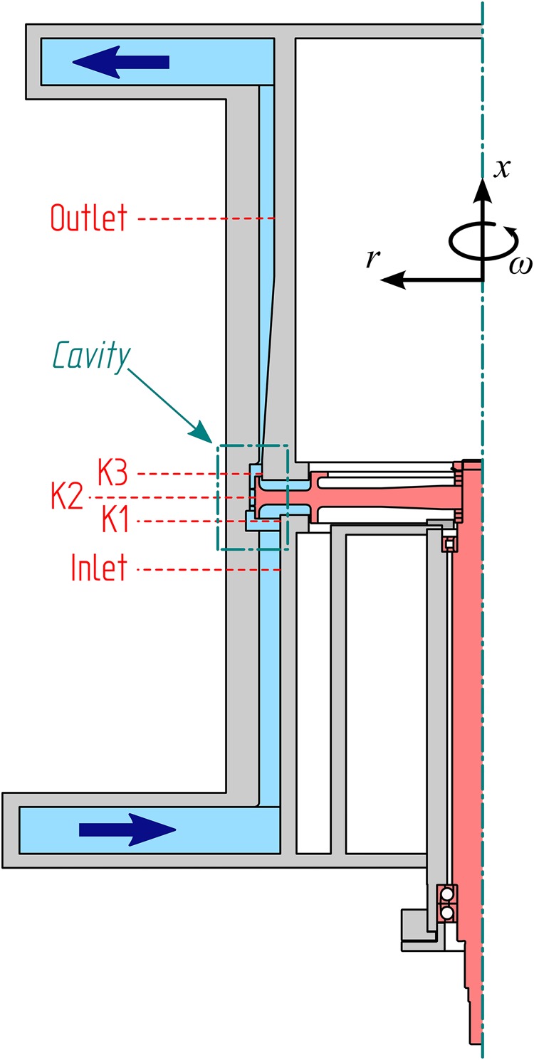
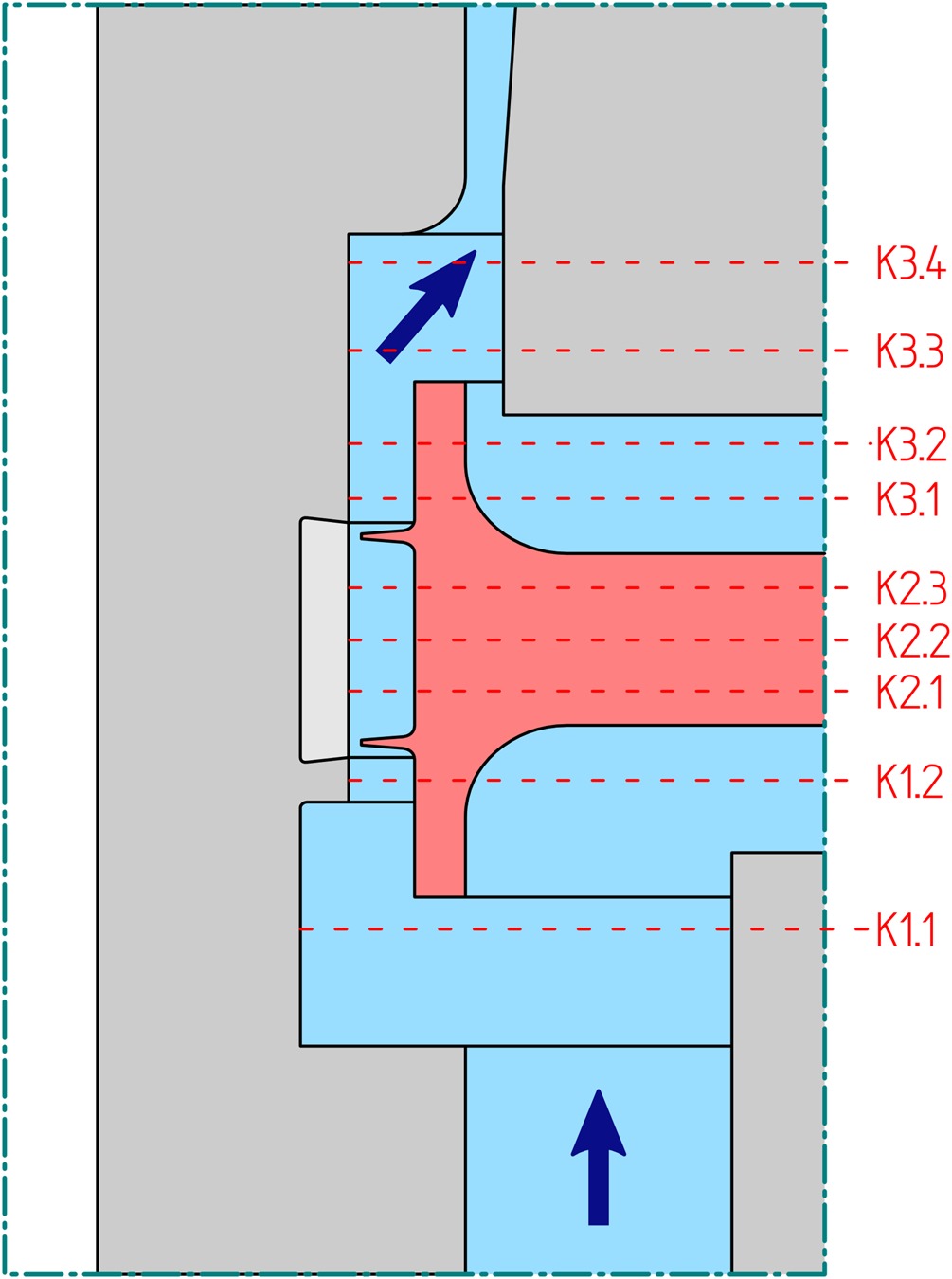
The inlet and outlet planes represent the beginning and end of the control volume in all CFD simulations. The boundary conditions are measured in these locations. The labyrinth seal cavity is subdivided into the cavity inlet (K1), swirl chamber (K2), and cavity outlet (K3), cf. Figure 1.

The entire test rig between inlet and outlet volute is rotationally symmetric. The flow path is free from obstructions such as struts to eliminate external excitation of unsteadiness.

Instrumentation

Detailed measurements of pressure and temperature are recorded in the cavity inlet (K1) and outlet (K3) as well as the swirl chamber (K2), cf. Figure 2. The instrumentation is listed in more detail in Kluge et al. (2019).

Figure 2.

Longitudinal section of the labyrinth seal cavity (cf. Cavity in Figure 1).

Total and static pressure as well as total temperature are measured in the inlet and outlet plane of the test rig. All data is recorded synchronously to provide the boundary conditions for the analysis of time-resolved pressure measurements.

To record unsteady flow phenomena inside the inlet and outlet cavities, both are instrumented with time-resolving pressure sensors (Kulite XCQ-062) in the axial positions K1.1 and K3.3, cf. Figure 2. Two circumferential locations are available in the cavity inlet spaced circumferentially 180° apart. Preliminary measurements have shown that no significant source of unsteadiness is present inside the cavity inlet. The cavity outlet is instrumented at α=0∘, 7.5°, 22.5°, and 57.5° circumferentially. An additional position at 180° is available. The operating point in the experiment is defined by the reduced mass-flow rate and the reduced rotational speed to obtain constant axial and rotational Mach numbers independent from ambient conditions.

Theory

The following kinematic model serves to explain the spectral footprint of the unsteady measurements reported in the results section of this paper. The spectrum found in the data shows periodic signal components, which are non-harmonic to the rotor frequency (as shown in an exemplary spectrum below). The model described here is referred to during the analysis of the data.

The model consists of rotating nodal structures. Multiple modes are superimposed while rotating at a common speed. The physical nature of the nodes themselves is arbitrary, however, in the present data they manifested as pressure fluctuations. An example of a single mode is shown in Figure 3. This structure consists of a distinct number N of pressure lobes equally spaced over the circumference (spacing β). It rotates at an angular speed ωs.

Figure 3.

Schematic of the rotating coherent structure with N=8 nodes, angular relations, and exemplary sensor positions.

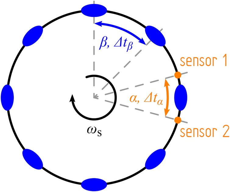
Inside the cavity, a minimum of two sensors are mounted, spaced at a given angle α. The frequency

may be detected in unsteady pressure traces recorded by both sensors. The time lag while one lobe passes through the angle β=(2π/N) is defined by

Accordingly, the time lag

defines the duration of the passage of one lobe through the angle α. The latter defines also the time shift between the two signals. The time lags Δtα and Δtβ are determined by cross-correlating the two signals.

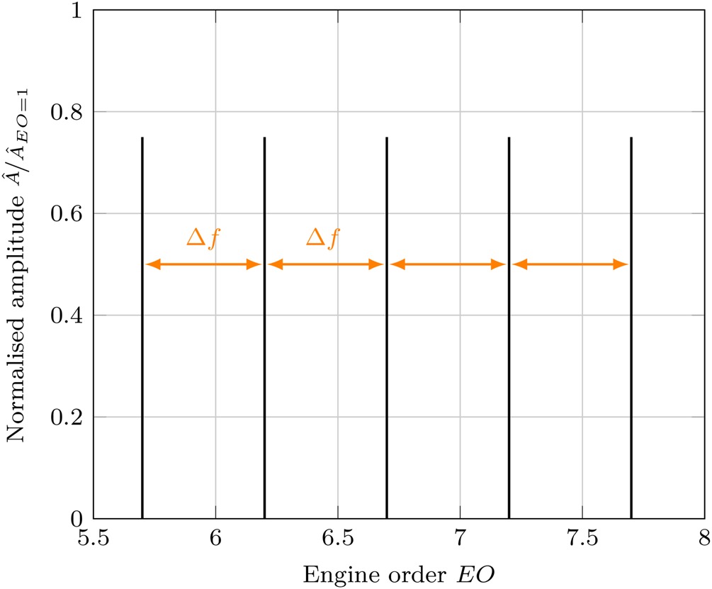
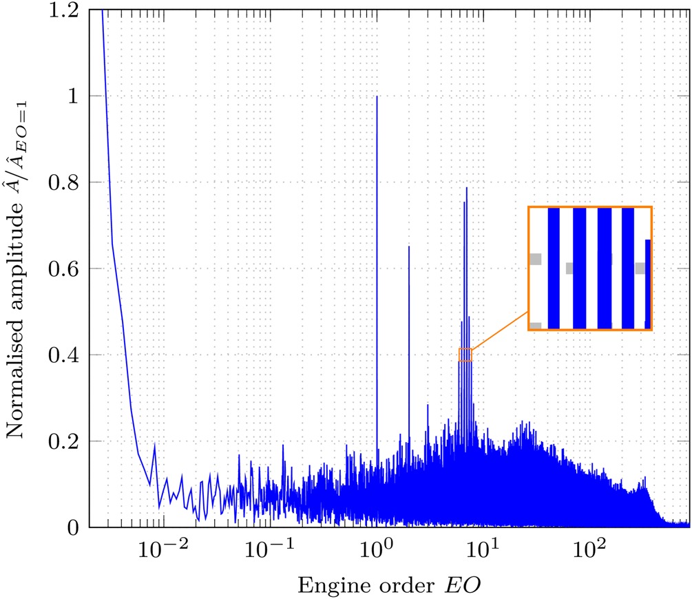
Rotating periodic structures cause a distinct frequency response. When multiple modes, which differ only in their number of pressure lobes Ni but not in ωs, are superimposed, the sensors detect a corresponding number of distinct frequencies. In this case, the amplitude spectrum of the signal trace shows peaks, which are evenly spaced by

where the individual frequencies are given by

An example of such a spectrum is given in Figure 4.

Figure 4.

Spectral response due to five superimposed nodal structures with Ni=N1+k rotating at a common speed ωs.

Methodology

The methods used for the analysis of data in this study are defined in this section. They are applied to experimental as well as numerical data. First, all data is low-pass filtered for anti-aliasing by a first-order Butterworth filter with a cut-off frequency of 90 kHz, i.e. less than half of the sampling frequency of 200 kHz. Second, spectral analysis of the data is performed by means of a fast Fourier transform with a von-Hann window function.

The number of nodes and rotational speed of individual rotating modes are identified by cross-correlating signals from different sensors. An example of the cross-correlation is given in Figure 5. To isolate individual modes, the signals are filtered by tenth-order Butterworth band-passes.

Figure 5.

Cross-correlation of filtered signal traces are used to determine parameters describing unsteady phenomena.

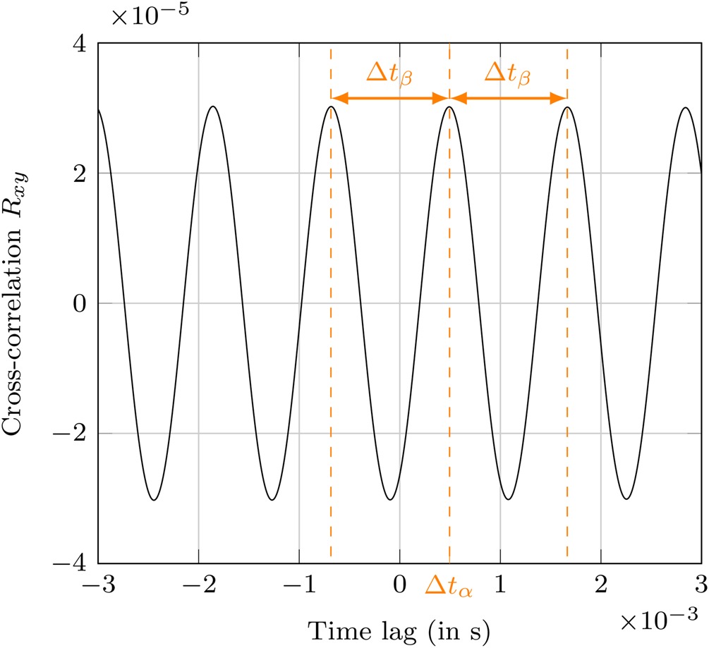
By cross-correlation, Δtα is determined as the first maximum to the right of the origin. Δtβ is equivalent to the time lag between two adjacent maxima (cf. Figure 5). In the case of large numbers of nodes or large angles between correlated sensors, i.e. α>β, erroneous readings occur. In this case, the true time lag of the two signals is given by

While Δtβ can be identified unambiguously in the cross-correlation results, the readings of Δtα may be ambiguous. The latter value must be confirmed by correlating decreasing angles between two sensors. It is most likely that the smallest spacing between two sensors gives the true value for Δtα.

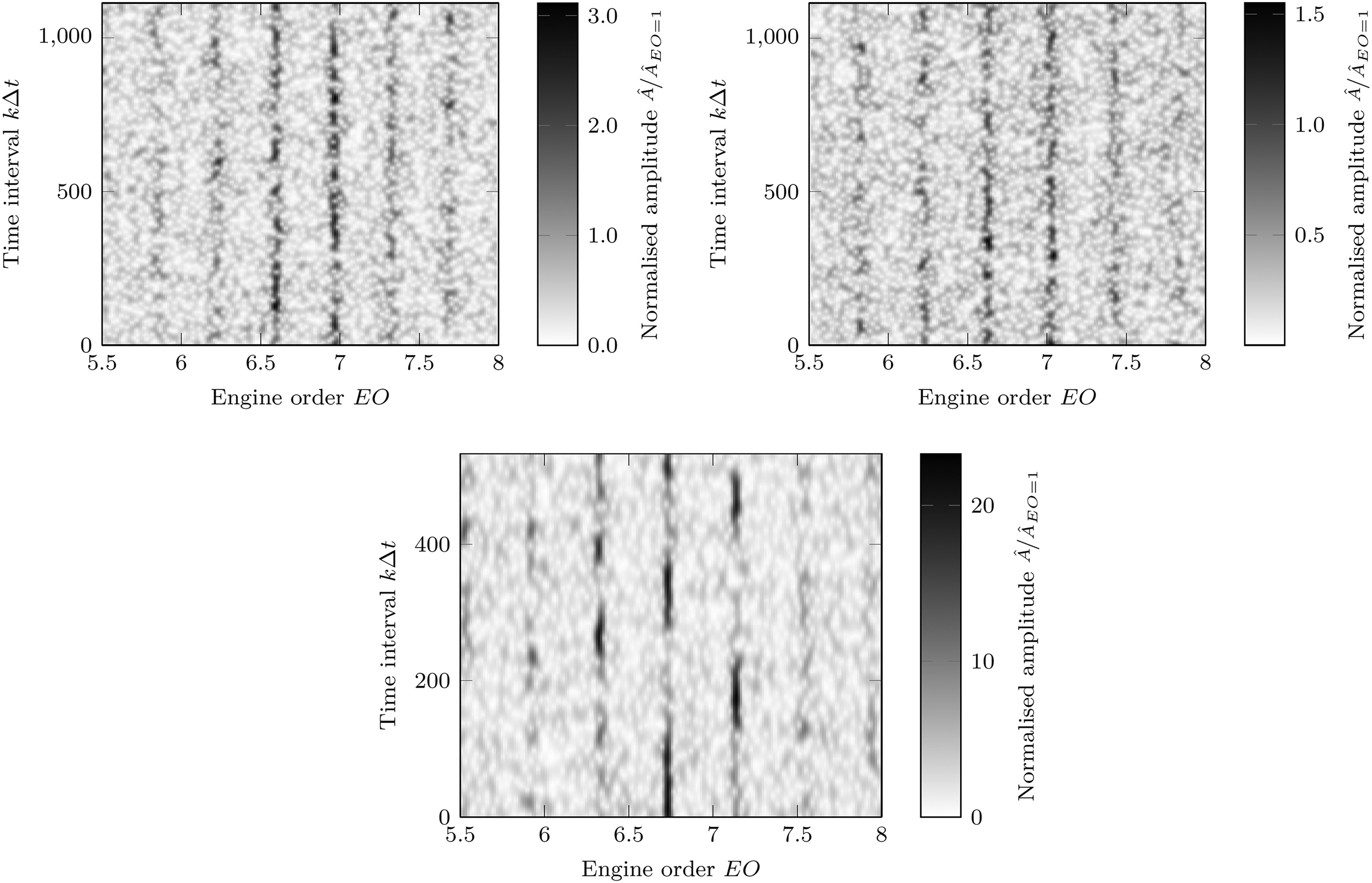
As indicated in the previous section, multiple modes with varying nodal numbers are superimposed to produce the spectral response found in the data. To determine whether truly synchronous superposition or varying nodal numbers occur, the variation of the spectrum over time is visualised in the form of waterfall diagrams. Ideally, a spectral analysis for each rotor revolution would be conducted. However, due to the high angular velocity, a sufficient resolution of the target frequency band cannot be achieved. Instead, the spectral analysis is performed for a sliding window of the signal trace. A length of 50 revolutions leads to a sufficiently fine resolution of Δf≈1.5Hz (cf. Equation 9).

In an effort to analyse the parameters influencing the occurrence of unsteady pressure fluctuations presented in the results, the theoretical axial velocity cax∗ of the flow inside the seal clearance is determined. To this end, the following approximations are necessary. The clearance is calculated a priori, taking into consideration the centrifugal strain of the disk at each operating point (cf. Kluge et al., 2019). Due to the constraint of the leakage jet by vortices forming in the labyrinth seal, the annulus area may be approximated by the area in the seal clearance. The temperature in the shroud area (K2.2) is approximated by the mean value of the temperatures inside the cavity inlet (K1.1) and outlet (K3.3). With the pressure and mass flow measured in situ, the theoretical incompressible velocity in axial direction may be calculated. The cavity flow coefficient

is defined, relating the theoretical incompressible axial velocity to the circumferential speed at the seal clearance. This parameter has proven to be well suited for characterising the unsteady flow field, as will be shown in further detail below. This parameter is not to be confused with the integral stage flow coefficient at the blading of a turbine.

Results and discussion

Measurement data of multiple operating points is available for analysis. The unsteady phenomenon, which is the subject of this study, is present in the spectrum at three operating points (cf. Table 1). A summary of all operating points, including those, which feature no unsteady fluctuations, is given in Table 2 in the appendix. In the first part of this section, the results of the aerodynamic design operating point (ADP) are presented in detail. The results for alternative operating points are presented more briefly further below, highlighting differences and common aspects of the rotating structures found.

Design operating point

Figure 6 shows the amplitude spectrum of one sensor in the cavity outlet at the design operating point. Various signal components are evident in distinct peaks in the spectrum. The peaks at the integer multiples of the engine order (EO) are associated with harmonic signal components caused by the revolving rotor. In the band of EO=5.5 to EO=8 there are multiple peaks that cannot be explained as easily and indicate unsteady and non-harmonic flow phenomena. A closer look at this frequency band reveals that these peaks are equidistantly spaced by Δf≈42.6Hz and form the distinctive pattern introduced above (cf. Figure 4). Each peak in the amplitude spectrum corresponds with one modal structure with a distinct number of nodes. Further analysis by cross-correlation shows the number of nodes varies from N=16 to N=21. The significance of this frequency response is evident, as the amplitude of the peaks is 40…80% of the amplitude at an engine order of unity. The spectral response of all three other sensor traces in the cavity outlet at K3.3 (Figure 2) is similar. Hence, the extent of this phenomenon is not spatially confined to one sensor location.

Figure 6.

Amplitude spectrum of one sensor in the cavity outlet at OP 1.

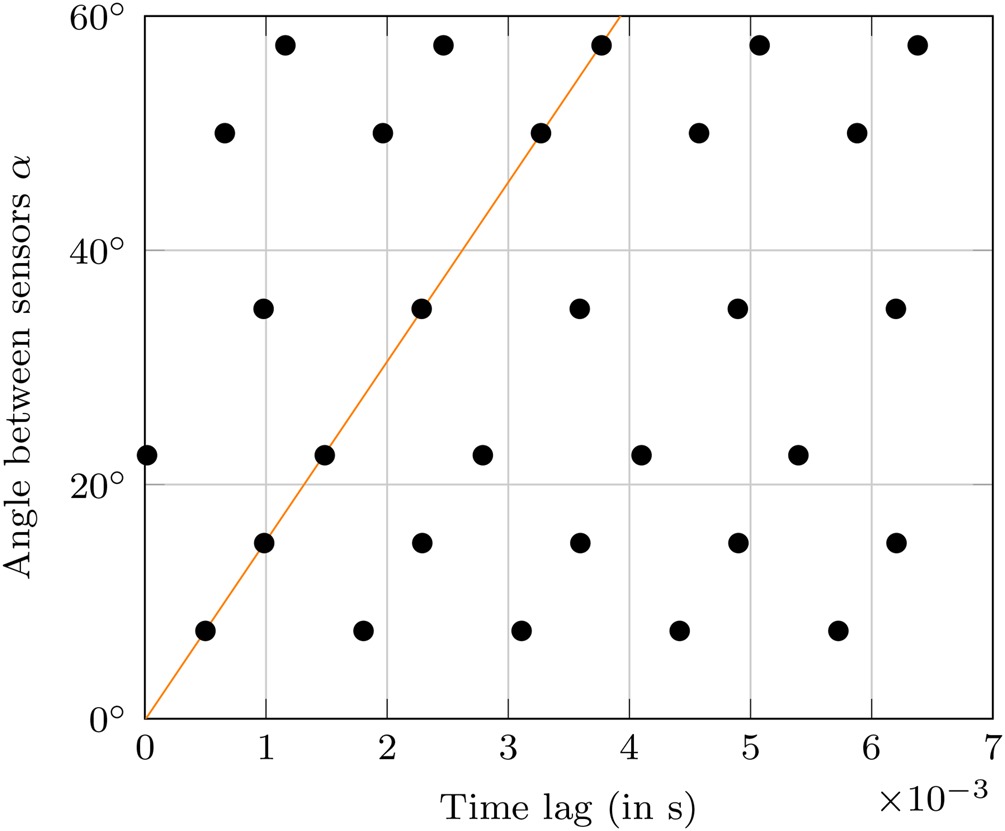
With the four sensors, six pairwise cross-correlation combinations are available to identify the rotating structures in the cavity. Figure 7 shows the results for one isolated peak in the amplitude spectrum at the ADP, i.e. for one of the superimposed nodal modes. The first five maxima to the right of the origin are plotted to account for the relation in Equation 7. Nevertheless, it appears plausible that the smallest sensor spacing yields the true result for Δtα. This interpretation is confirmed by the high correlation coefficient R2=1 of the regression function added to the plot. The slope of the regression function itself is equivalent to the angular speed of the mode ωs≈0.365Ω. Thus, the coherent structures found in this study rotate at a significantly lower relative speed than those in rim seals reported in open literature.

Figure 7.

Cross-correlation results for the signal component in the amplitude spectrum of the ADP at EO=6.6.

The development of the rotating structures over time is analysed in a waterfall diagram in Figure 8. Five vertical lines are distinctly identifiable, which correspond to the frequency pattern in the amplitude spectrum in Figure 6, i.e. the rotating structures featuring different numbers of nodes as identified by cross-correlation. The data at operating points 1 and 2 suggests that multiple modes are superimposed. For operating point 3, the data appears to suggest that only one mode is present for each point in time with the number of nodes varying. This would suggest a periodic breakdown and re-forming of these structures.

Figure 8.

Waterfall diagrams of OP 1 (ADP) with Δt≈0.43s (top left), OP 2 with Δt≈0.43s (top right) and OP 3 with Δt≈0.86s (bottom).

Influencing parameters

The previous discussion focused on operating points at which the described flow phenomenon occurs. It was found, however, that not all operating points actually feature this unsteady flow structure. Furthermore, no such pressure fluctuations are measured in the cavity inlet at any operating point precluding a causal link of the unsteadiness in the cavity outlet to upstream effects. Spectral analysis of accelerometer signals recorded at the rotor bearings eliminates vibrations as a source for the unsteady signals.

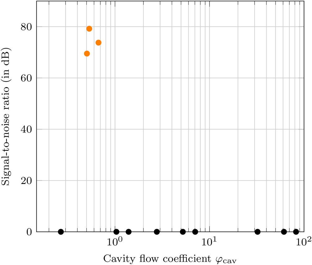
As depicted in Figure 9, the occurrence of unsteady flow structures in the outlet cavity appears to be dependent on the cavity flow coefficient φcav. As discussed above, the axial velocity cax∗ is not measured directly; it is a theoretical value instead. The operating points at which the unsteady flow phenomenon does occur, feature a velocity ratio between φcav=cax∗/U≈0.5…0.75. For operating points with φcav>1, the unsteady fluctuation is apparently suppressed. A lower boundary appears to exist as well as indicated by the operating point with φcav=0.28. The signal-to-noise ratio, as well as the relative rotational speed ωs/Ω are remarkably similar for all operating points investigated. The noise level is determined by eliminating the deterministic signal components by deconvolution (Kluge et al., 2015) of the signal. Thus isolating the deterministic components, the stochastic components of the signal remain. From those, the noise level is calculated as the root mean square of the stochastic signal components.

Figure 9.

Signal-to-noise ratio as an indication of the presence of the unsteady flow regime.

Numerical simulation

Similar flow phenomena are observed in URANS simulations of the test rig. To compare the experimental and numerical results, the unsteady pressure is analysed at monitor points identical in position to the unsteady pressure sensors in the experiment. Figure 10 shows the amplitude spectrum of the unsteady pressure at operating point 1. There are several distinct peaks in the frequency band of EO=5…7.5, forming a similar frequency pattern to the experimental data presented in Figure 6. The distance between two peaks is approximately 46.3 Hz compared to 42.6 Hz in the experimental data. Additional patterns can be seen at EO=11…14, 17…20, and 23…26, though much lower in intensity. As these are multiples of the EO of the non-harmonic pressure fluctuation it is likely that they are higher-order harmonics of this structure.

Figure 10.

Amplitude spectrum of the numerical simulation at ADP (monitor point location identical to actual probe).

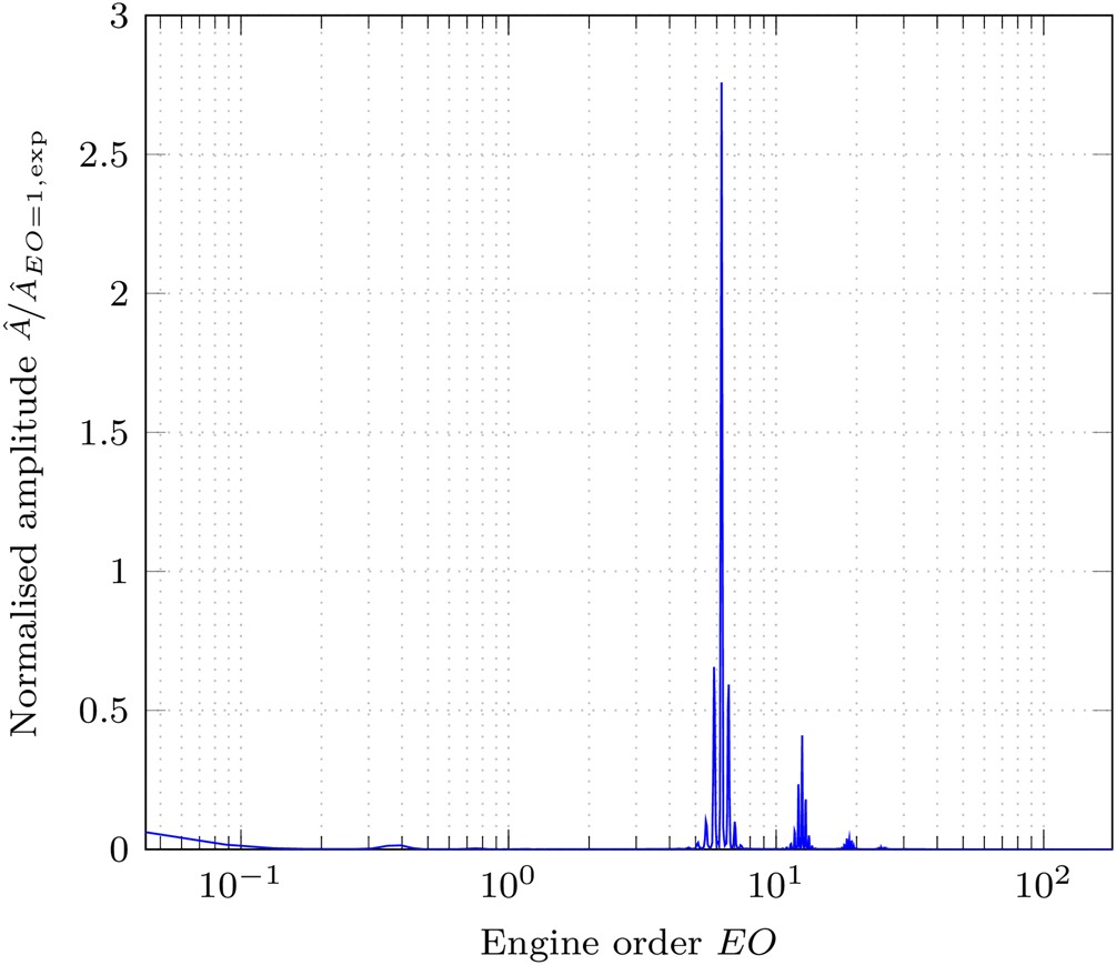
The amplitude is more than three times higher than that of the experiment. It is important to note that the numerical set-up describes a perfect rotor without eccentricity or other imperfections, which is why no peak at EO=1 exists.

The results of the cross-correlation for the peak at EO≈6.6 is displayed in Figure 11. From the cross-correlation, the number of nodes is derived as N=16 and the structure is rotating at ωs≈0.39Ω. The angular velocity is over-predicted by 7% compared to the experimental data while the number of nodes is in the range of the experimental results. It is important to note, however, that the accuracy of the cross-correlation is limited due to the comparatively lower sampling frequency, i.e. the time step of the simulation.

Figure 11.

Cross-correlation of the pressure signal from the URANS simulation of the ADP for the signal component at EO=6.6 with a linear regression correlation coefficient R2=0.9997.

Conclusions

Unsteady pressure fluctuations are observed in the outlet of a labyrinth seal cavity modelling a tip cavity of a shrouded turbine. These fluctuations are non-harmonic to the rotor speed and a kinematic model can be used to explain the spectral signature of the phenomenon. The fluctuations are similar to observations in rim seal cavities reported in literature. Based on the data at hand, no certain conclusion with regard to the aerodynamic cause, e.g. Taylor-Couette vortices or Kelvin-Helmholtz instabilities, may be drawn. Shallow cavity modes may be eliminated as the source of the unsteadiness based on the linear frequency pattern in the amplitude spectrum. Additionally, mechanical vibration of the rotor is ruled out as the cause of the unsteady pressure.

The occurrence of the unsteady pressure fluctuations is shown to depend on the cavity flow coefficient φcav defined in this paper, i.e. the ratio of a theoretical axial velocity of the leakage flow and the circumferential velocity of the shroud. The fluctuations are present in the signal spectrum only while this flow coefficient is in a narrow range of approximately 0.5 to 0.75. Additional measurements and simulations are required to confirm and narrow down the limits of this range.

URANS simulations are shown to reproduce the pressure fluctuation. The spectral signature is very similar to the experimental data. There are small discrepancies in the number of nodes and the angular velocity at which the modes rotate. The discrepancies may be due to the limited sampling frequency defined by the time step of the numerical simulation. Additionally, the frequency resolution may be improved by longer simulations.

Future CFD simulations of additional operating points will serve to confirm or contradict the dependency of unsteady pressure fluctuations in the labyrinth seal cavity outlet on the ratio of axial flow velocity and rotational speed of the shroud. If confirmed, the phenomenon may be analysed further for the underlying aerodynamic causes of the fluctuation based on the simulations. A forthcoming publication will show that LES simulations are even more suitable for modelling the physical phenomena described in the present publication than RANS-based CFD.

Nomenclature