
Introduction
As the spatial resolution and internal calibration stability of IR cameras has improved, they have become more popular as research instruments in the gas turbine heat transfer community. It is common practice to calibrate the camera (IR radiometric value) against a region of known temperature (typically by thermocouple measurement) in the field of view (FOV) of the camera. The in situ calibration, whilst typically having the disadvantage of less accurate surface temperature measurement (thermocouple instead of RTD, as it would be common in dedicated calibration instruments), has the significant advantage of directly accounting for poorly characterized target surface emissivity, angle variation and transmissivity of elements in the optical path (windows in pressure vessels typically being the most significant). This is the prime reason for it being the most common method for target surface temperature evaluation (over methods involving separate out-of-experiment calibrations, and associated correction methods). Typical methods for instrumenting the target surface include embedding a thermocouple in the surface, or adhering it to the surface by means of an adhesive layer. Data is acquired simultaneously from both the IR camera and the thermocouple at a fixed location in space (i.e. fixed pixel location for the IR camera), resulting in a direct calibration for the target surface. Any thermal resistance (an adhesive layer, for example) between the thermocouple and the target surface will lead to a measurement error by the thermocouple in situations where there is through-wall heat flux. The presence of an adhesive layer will also cause a lateral temperature disturbance locally near the thermocouple junction. This complicates the formation of an accurate calibration curve, because of the high sensitivity to the selection of the thermocouple junction location (often just a few pixels wide) in a region of high lateral temperature variation. Additional uncertainty in the calibration chain can arise if an adhesive layer forms on the outer face of the thermocouple during its installation, due to the thermal resistance between the thermocouple junction and the surface being visualized. Indeed, a similar effect is often deliberately introduced in the form of a thin paint layer, in an effort to render the entire surface of uniform emissivity.
Literature relating to practice for IR calibration experiments
In the case of highly non-uniform wall heat transfer and surface temperature gradients (typical of, for instance, film cooling environments), high spatial resolution is required to fully characterize the complex thermal field. IR thermography is a perfect candidate for this type of applications as it offers both high spatial and thermal resolution. The accuracy of quantitative IR measurements relies on calibration experiments performed to correlate the radiometric signal from the camera to a known temperature. In turbine research environments (namely, represented by wind tunnels operating at either low- or high-speed conditions, with surface temperature variations), bespoke in situ experiments are required to calibrate the IR camera at the nominal test conditions. In situ tests are performed to correct for poorly characterized target surface emissivity, view angle variation, and transmissivity of elements in the optical path.
It is common practice when carrying out in situ calibration tests to compare the radiometric data to a thermocouple temperature at the thermocouple location in the IR image. A number of thermocouples are therefore embedded or bonded to the surface with an adhesive layer, and the temperature measured by the thermocouples used for calibration should cover the complete temperature range of interest.
Martiny et al. (1996) presented an in situ calibration technique for quantitative infrared measurements. The raw detector signal from the infrared camera was compared to the temperatures measured with thermocouples. The function between raw detector value and object temperature was cast in the form of the Plank equation. The latter included three parameters, which were used for a best-fit approximation. The resulting non-linear system of equations was solved numerically and the calculated parameters were used to estimate the corrected temperature of the body.
Schulz (2000) presented a quantitative infrared approach applied to film cooling research. Their work described the theoretical aspects and methods related to in situ calibrations. Examples of film cooling investigations using infrared thermography were also presented. In their experiments, a number of thermocouples were embedded in the surface and used to directly calibrate the radiometric signal from a single IR camera.
Ochs et al. (2009) proposed a technique to overcome the issue related to thermocouples being located in regions of high surface temperature gradients. The technique allows for data extrapolation with improved accuracy when calibrating the radiometric data to the thermocouple temperature. The approach was based on the determination of three of four calibration parameters by a pre-calibration run and a subsequent in situ calibration to estimate the value of the fourth parameter. They claimed that fewer thermocouples were necessary for the in situ calibration, and that thermocouples did not have to cover the entire temperature operating range (making therefore possible to discard the thermocouples located in regions of high temperature gradients). The method was applied to the thermal investigation of transonic trailing edge cooling and film cooling of a flat plate.
Despite the conspicuous number of papers on the application of IR thermography on film cooling research, we can find no mention of the effect of the calibration arrangement on the accuracy of surface temperature measurements. As it will be shown later, there is a strong sensitivity of the primary sources of error in the calibration to variations in the parameters involved in the measurement setup. In fact, various parameters such as adhesive/paint thickness and thermal conductivity substantially affect the temperature measured by the thermocouple and therefore can lead to increased overall uncertainty in the calibration process.
This paper presents a parametric study on the influence of the measurement layout on the temperature measured by the thermocouple. The influence of a number of physical parameters is assessed in the context of their effect on the difference between thermocouple temperature measurement used for calibration and the temperature of the surface seen by the IR camera. A new instrumentation methodology is proposed which has significant advantages over more conventional methods, in that it mitigates the primary sources of error. The method offers a low thermocouple measurement error in the presence of through-wall heat flux and a high accuracy in localizing the reference thermocouple in regions of high surface temperature gradients. In the proposed layout, a low conductivity substrate is implemented to locally minimize the through-wall heat flux, and a high thermal conductivity layer is bonded to a thermocouple by means of thermally conductive paste. The high conductivity layer is designed to operate at low values of the Biot number, namely that uniform spatial temperature is reached during the test. An area including several pixels at uniform temperature is therefore available in the IR image, leading to substantially reduced error when calibrating the radiometric signal to the true wall temperature measured by the thermocouple.
It is hoped that results from this paper will be useful to researchers to understand the influence of the physical parameters involved in the calibration experiments, and to quantify the systematic primary error introduced by the system layout in the surface temperature measurement.
Assessment of errors associated with conventional measurement systems
We now consider typical errors in the most common thermocouple temperature measurement and calibration systems. This discussion is progressed under two headings: sensitivity of surface temperature measurement to adhesive and paint layers; and sensitivity of surface temperature measurement to pixel selection in regions of high temperature gradient.
Sensitivity of surface temperature measurement to adhesive and paint layers
In this section, we assess the sensitivity of the surface temperature measurement to the structure of the surface measurement system. In particular, we consider the effect of adhesive and paint layers on the temperature measured by the thermocouple. We use a one-dimensional steady-state heat transfer model to consider the impact of thermal conductivities and thickness of such layers in a number of common surface measurement systems.
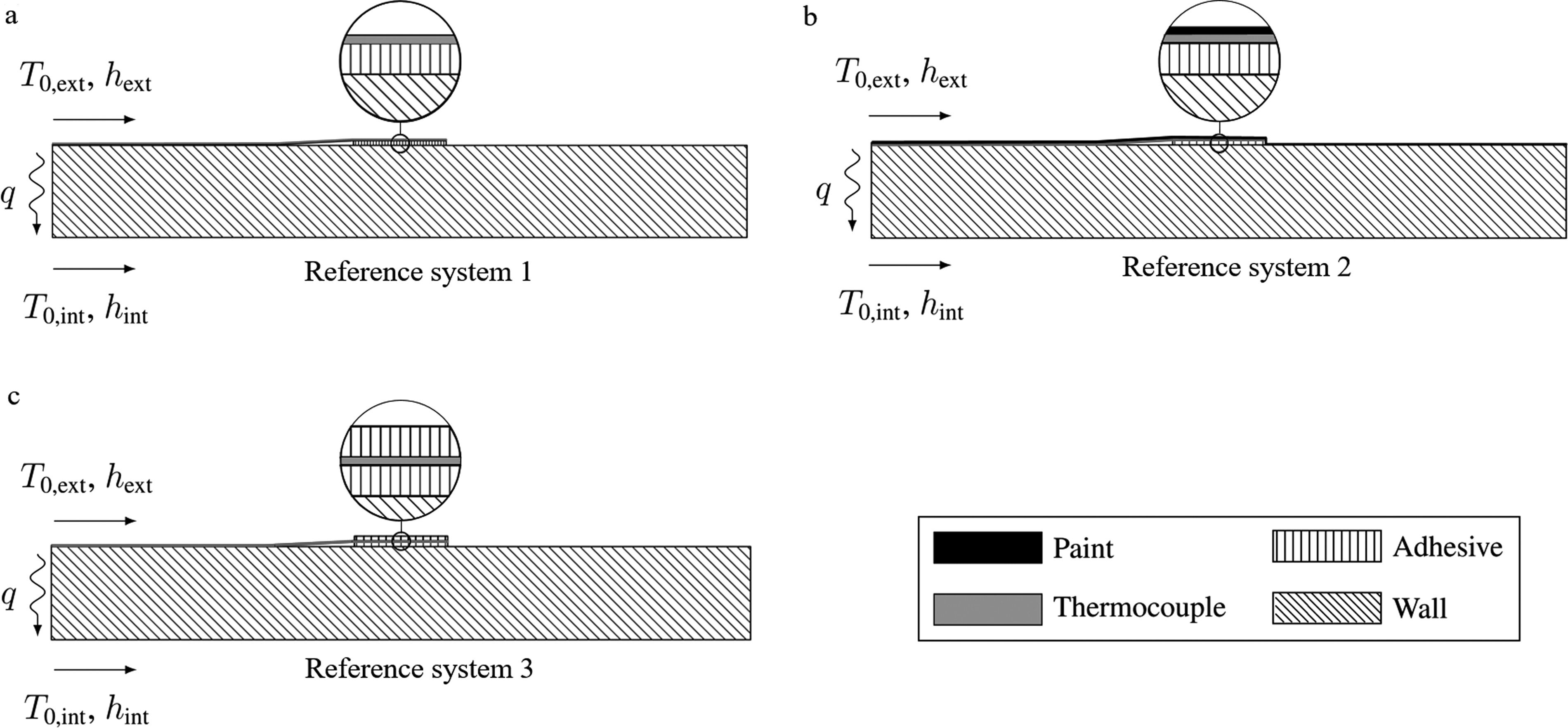
Figure 1 shows three conventional surface measurement systems used for in-situ IR calibration. We refer to these as reference systems 1 to 3. The systems are: (1) thermocouple over adhesive; (2) over-painted thermocouple over adhesive; (3) thermocouple between adhesive layers. Reference system 1 is representative of a typical foil thermocouple (used to minimise surface aero-thermal disruption) adhered directly to a surface. Reference system 2 is a modified version of system 1, in which the foil thermocouple is additionally over-painted to render the surface of uniform emissivity. Reference system 3 represents a foil thermocouple that is adhered between adhesive layers (sometimes used either for robustness, or arising due to unintentional over-coating with glue when adhering with resin-based glue).
Figure 1.
Diagrams of the reference systems (scale 4.5:1): (a) thermocouple over adhesive; (b) over-painted thermocouple over adhesive; (c) thermocouple between adhesive layers.
In the analysis of these systems, the wall is subject to a (hot) external flow at total temperature
Table 1.
Wall boundary conditions.
Table 2.
Wall thermal properties.
| Property | Symbol | Value |
|---|---|---|
| Wall thickness | 1.50 mm | |
| Wall conductivity | 11.7 W m−1 K−1 |
In the analysis of these systems, we differentiate between three types of measurement error: (1) error between the thermocouple measurement and the surface temperature directly above the thermocouple junction; (2) error between the thermocouple measurement and the surface temperature near the thermocouple junction; (3) the error between the thermocouple measurement and the true undisturbed wall temperature (without the presence of the thermocouple, or any associated surface treatment, for example thin over-paint layers). Errors of type 1 are the direct error arising in the calibration process when selecting a pixel directly above the thermocouple junction to compare against the thermocouple data. This error is intrinsic in all calibration processes and is difficult to remove. Errors of type 2 arise when there is lateral surface temperature variation, when either the selected pixel in the IR image is not the one directly above the thermocouple junction, or where there is a requirement to average a region in the vicinity of the thermocouple. Errors of type 3 (between the thermocouple measurement and the true undisturbed wall temperature) are most relevant for thermal analysis of a particular component, when the effect of all instrumentation (including thin paint layers) must be accounted for.
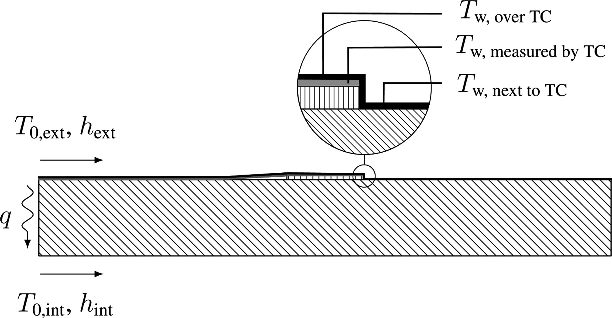
These errors, presented in a form normalised by the total temperature difference between the streams, are defined by Equations (1)–(3). The temperatures used in these definitions (except for the true undisturbed wall temperature) are defined in Figure 2. In this paper we are concerned with measurement errors of type 1 and 2
Reference system 1: thermocouple over adhesive
Since the thermocouple junction in reference system 1 (Figure 1a) is exposed (not covered by paint or adhesive), the measured temperature by the thermocouple is the same as the temperature directly above the thermocouple junction. Therefore, reference system 1 is not affected by errors of type 1; i.e.
In the presence of through-wall heat flux, the adhesive layer underneath the thermocouple causes errors of type 2
Figure 3 presents
Figure 3.
Analysis of reference system 1, showing β
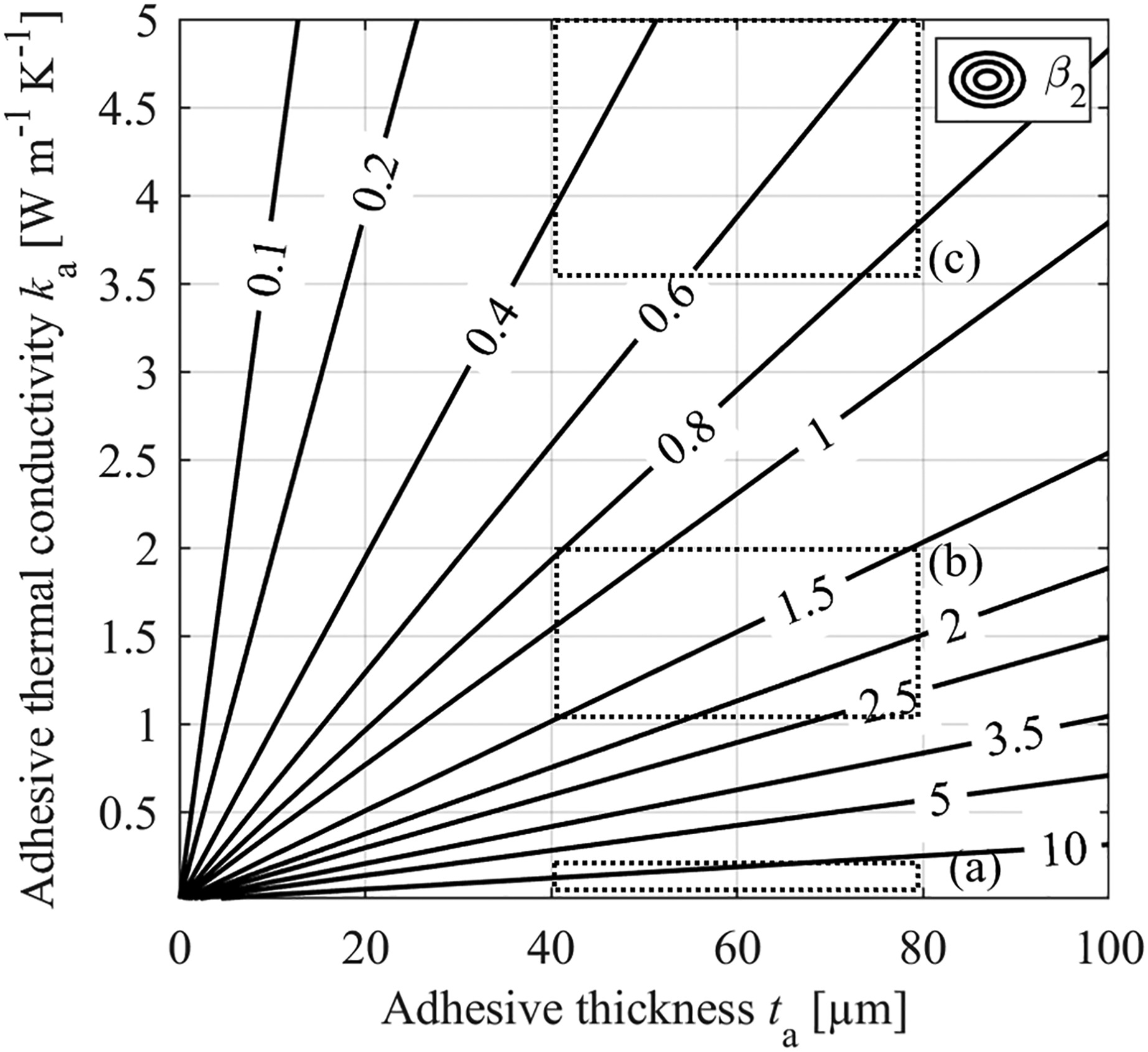
A foil thermocouple with a standard epoxy bonding layer would typically have an adhesive layer thickness of 40.0–80.0 μm. Although epoxy adhesives offer a high bonding strength, typical thermal conductivities of these adhesives are very low: typically in the range 0.100–0.200 W m−1 K−1 (Lee and Neville, 1967). This range of values is marked in the figure as (a). For the through-wall heat flux conditions considered (Table 1), the error for the worst-case estimated values of thermal conductivity and layer thickness can be up to 20.0% of the total temperature difference between the streams. Even at the best-case end of the estimated range errors of 7.0% are likely. It is clear that using instrumentation systems of this type it is necessary to be extremely careful with installation effects. Even so, using such systems for high-accuracy calibration systems would appear to be a risky proposition.
An alternative option would be to use a thermally conductive epoxy, which has a thermal conductivity in the range 1.00–2.00 W m−1 K−1. This situation is marked as (b) in the figure. Even for thermally conductive epoxy, the estimated range of errors is between 0.80 and 3.00% of the total temperature difference between the streams. Although the use of high conductivity epoxy partially mitigates the errors arising in high through-wall heat flux situations, errors can still be high in the context of high accuracy calibration requirements.
An improved option might be to use a high thermal conductivity (and low electrical conductivity) adhesive. Such adhesives would typically also have a bonding layer thickness in the range 40.0–80.0 μm, with a thermal conductivity in the range 3.50–5.00 W m−1 K−1. This range of values is marked in the figure as (c). For best-case estimated values of thermal conductivity and layer thickness, the error is estimated to be at least 0.30% of the total temperature difference between the streams. The measurement error can be up to 0.90% for the worst case. However, the typical tensile strength of high thermal conductivity adhesives is considerably lower than standard epoxy resins (1.00–2.00 MPa, versus more than 20.0 MPa for common epoxy resins) and this is a serious consideration in high-speed flow environments.
Reference system 2: over-painted thermocouple over adhesive
It is a common practice in IR thermography to spray a thin layer of paint over the entire target surface (including the reference thermocouple) to render the surface of uniform emissivity. This situation is shown in Figure 1b. In the presence of through-wall heat flux, the over-paint layer acts as an additional thermal resistance, and raises (for higher mainstream gas temperature) the surface temperature (visualised by the IR camera) with respect to the thermocouple measurement. This leads to errors of type 1. The effect is rather different to that of underside adhesive, which raises both the thermocouple temperature and the wall temperature above it, leading to errors of type 2 where pixels near to, but not directly above the thermocouple are considered as part of the calibration process. Because nearby pixels (not over the adhesive layer on which the thermocouple is mounted) would tend to register lower temperature in an IR image, the type 2 error is generally of opposite sign to the type 1 error.
Matt black acrylic paint is commonly used in IR thermography, and has a thermal conductivity in the range 0.500–1.50 W m−1 K−1 (Raghu and Philip, 2006). With well-controlled spraying, a layer thickness as low as 10.0 μm is possible. Figure 4 presents errors of type 1 and 2 (
Figure 4.
Analysis of reference system 2, showing β β
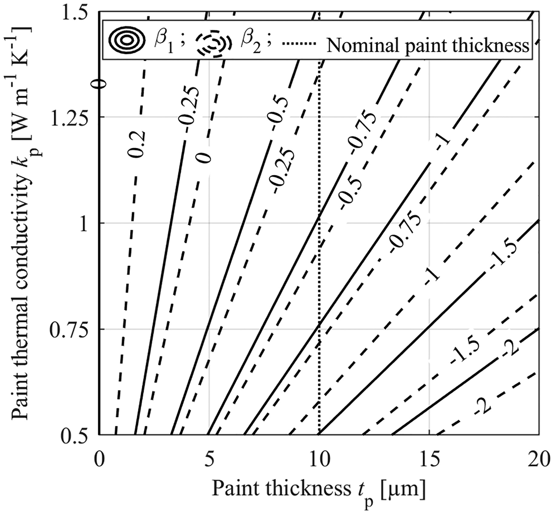
Figure 4 shows type 1 and type 2 errors,
Reference system 3: thermocouple between adhesive layers
During the thermocouple installation a layer of adhesive can form over the thermocouple junction, adding further thermal resistance. Figures 5 and 6 show the contours of
Figure 5.
Analysis of reference system 3, showing β
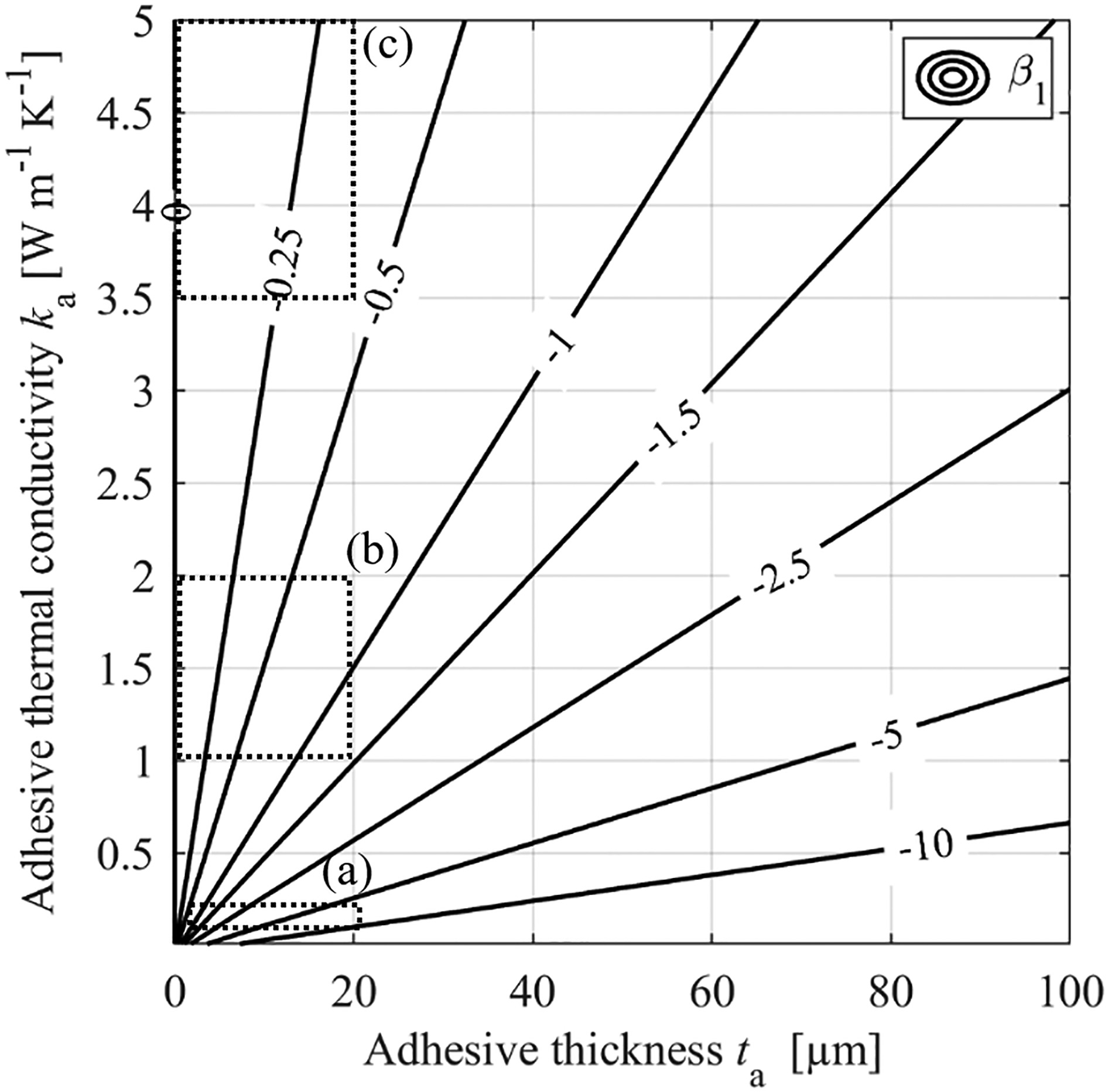
Figure 6.
Analysis of reference system 3, showing β

Adhesive over the thermocouple has the effect of introducing error between the local (directly above the thermocouple) external wall temperature and the thermocouple temperature, and is a cause of
So far as
A typical adhesive layer thickness over the thermocouple can be up to 20.0 μm. For standard epoxy adhesives (region marked as (a) in Figure 5), the direct calibration error
Concerning
We numerically assessed the dependency of the thermocouple temperature on the measurement layout and physical properties of the adhesive used. We observed that the measurement error strongly depends on the location, thickness and thermal conductivity of the adhesive layer in the presence of through-wall heat flux. In practice, poorly characterized adhesive/paint thermal properties and thicknesses could lead to significantly large measurement errors and increased overall calibration uncertainty.
Sensitivity of surface temperature measurement to pixel selection in regions of high temperature gradient
To calibrate IR camera output to a measured wall temperature, radiometric values are recorded against thermocouple readings. In this process it is required that the thermocouple reading is as representative as possible of the local surface temperature. If the region of the thermocouple is sufficiently isothermal, the temperature directly above the thermocouple location can be taken. Errors for this situation have been discussed. Where the surface is non-isothermal—on account of disruption by the thermocouple system for example—the error associated with region selection must also be considered. In this case, two errors must be considered: the error between the thermocouple and wall temperature directly above the thermocouple
When IR images are taken, it is typical to select a region of several pixels around the thermocouple junction location to establish an area-averaged radiometric value on the target surface. Moderate lateral temperature gradients are possible because of the nature of the components being studied, as shown, for example in the results of Kirollos et al. (2017), which are reproduced in Figure 7. The figure shows a nozzle guide vane non-dimensional surface temperature presented as overall cooling effectiveness θ (the complete definition of θ is described in Kirollos et al., 2017). The part was fully cooled (both external film and internal convective cooling) and was operated at conditions non-dimensionally representative of an engine. In these demonstration measurements, a thin foil K-type thermocouple was used (indicated in Figure 7) to calibrate IR data. The thermocouple installation scheme was like reference system 2 (Figure 1b): over-painted thermocouple over adhesive.
Figure 7.
Example of overall cooling effectiveness (θ
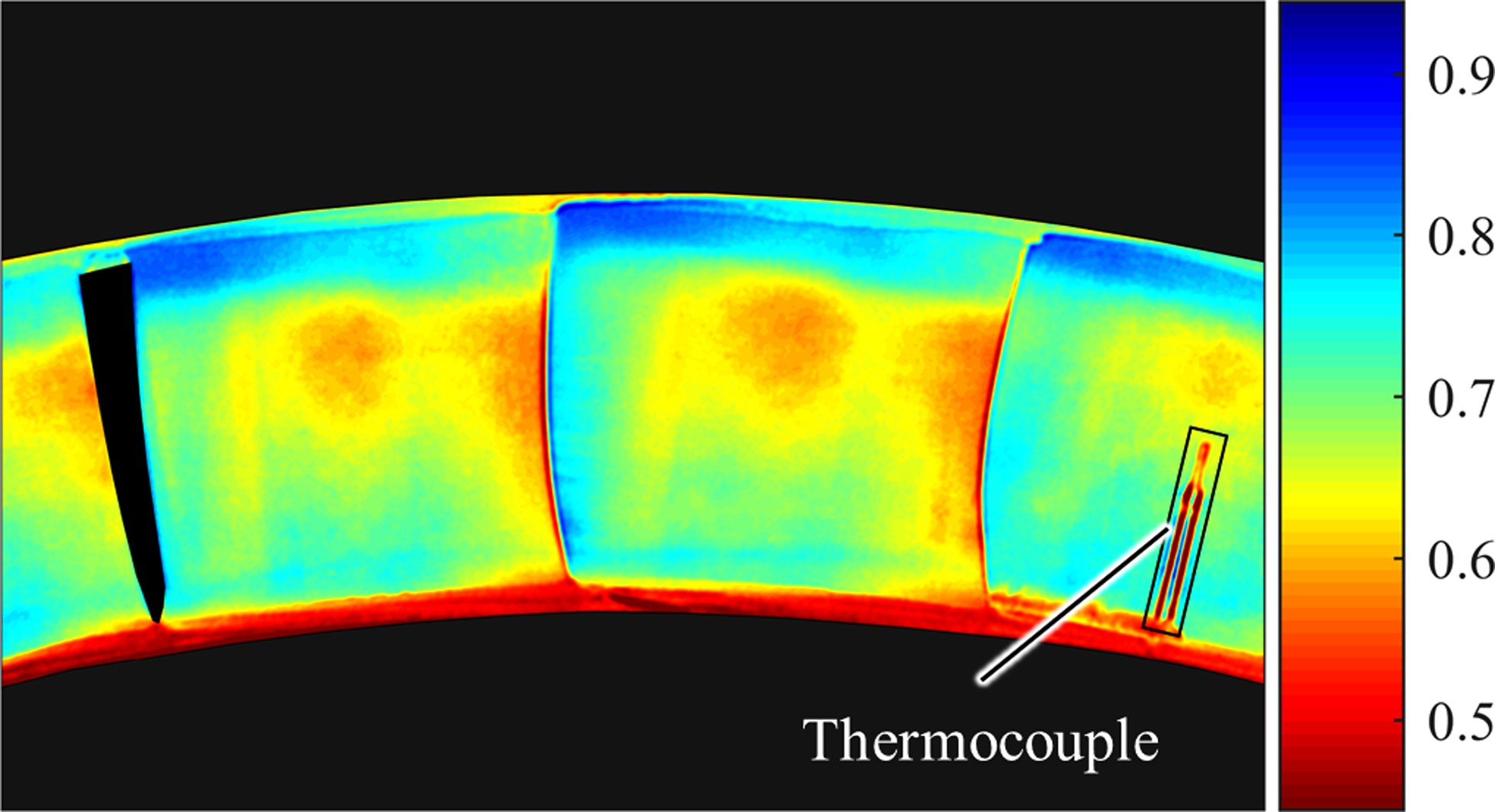
The thermocouple wires are visible in Figure 7 because of the change in surface temperature due to the variation in thermal resistance with respect to the undisturbed surface. This primarily results from a thin layer of epoxy under the leads.
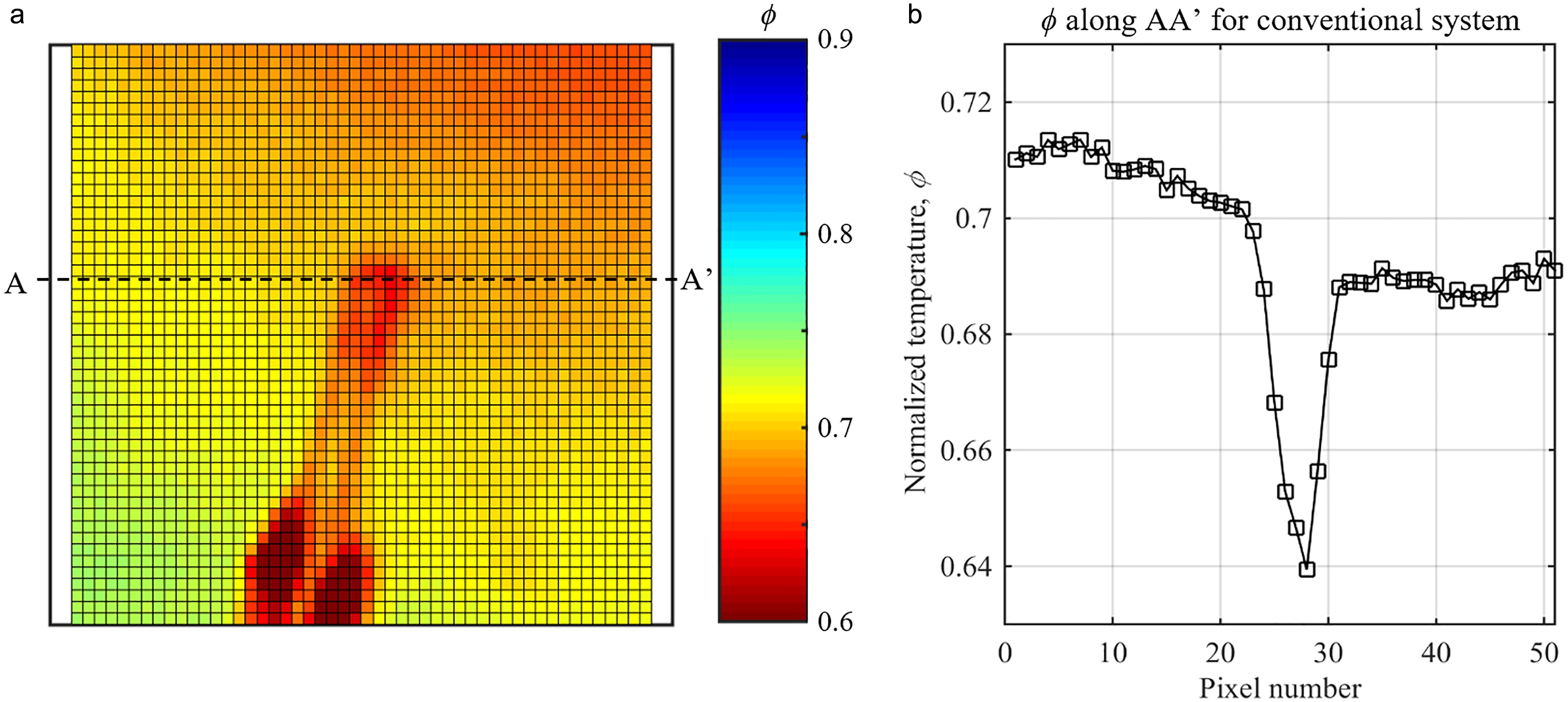
A detail view of the results of Figure 7 is presented in Figure 8a in terms of normalized temperature
Figure 8.
Conventional calibration system (reference system 2): (a) surface plot of ϕ ϕ
where
It is clear that the moderate lateral temperature gradients on the vane surface are compounded by high temperature gradients local to the thermocouple, caused by the disturbance of the thermocouple construction.
This is emphasized by Figure 8b, which shows the lateral distribution of normalized temperature along the line AA′ through the thermocouple junction. Individual points represent single pixels in the IR image. Significant lateral temperature variation is apparent. This situation is very common even with the most careful instrumentation scheme. In this example it is clear that two sources of error must be considered. To reiterate: we must consider the error between the thermocouple measurement and wall temperature directly above the thermocouple junction
Proposal for an improved measurement system
We now propose an improved measurement and calibration system (for in situ IR calibration) optimised to reduce measurement error in environments with significant through-wall heat flux and/or lateral temperature gradient. The proposed system is shown in cross-section in Figure 9. We refer to this as reference system 4.
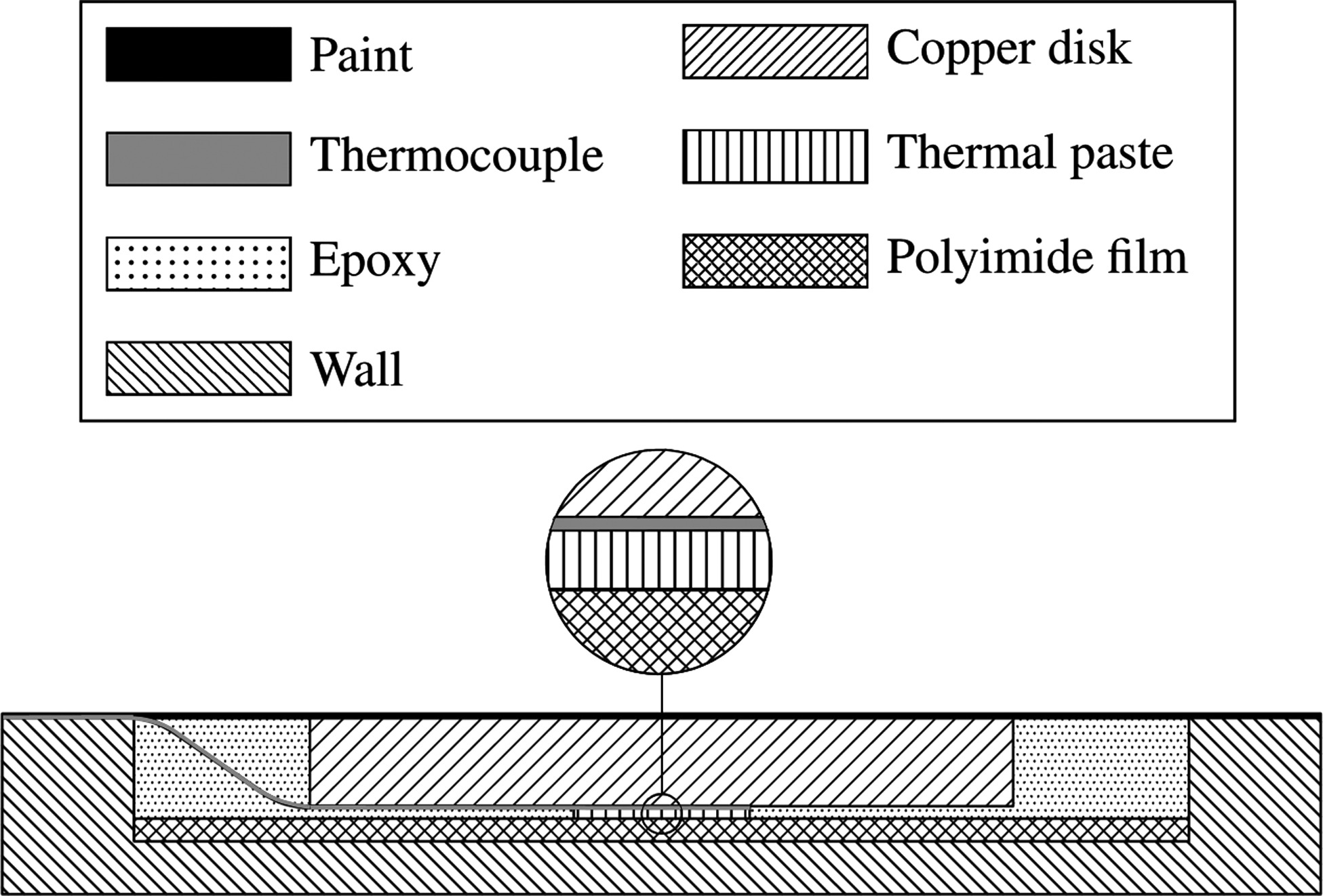
In the assembly, a thin-foil K-type thermocouple is bonded between a disk of copper (high thermal conductivity) and a polyimide film (low thermal conductivity). The thermocouple is in direct contact with the bottom face of the copper disk and a layer of thermal paste is applied under the thermocouple and on its sides to adhere it to the copper disk. The copper disk is held in place using an epoxy adhesive and the whole assembly is installed at the trailing edge of the vane—a region of low surface curvature—and is arranged flush with the surface to minimize boundary layer disruption. A layer of matt black paint is applied over the calibration and the target surfaces to render them of uniform and equal emissivity. Figure 10 is a photograph (plan view) of the system assembled on the suction side of a HPNGV before over-painting. The cavity into which the assembly was assembled was machined using a 6 mm diameter flat-bottom cutter to a depth of 0.7 mm. The copper disk is 4 mm in diameter and is 0.5 mm thick. The disk geometry can be scaled to suit the application. In situations where wall thickness is limiting, where there are high lateral gradients of mainstream gas temperature, and where the surface area of the sensor cannot be sufficiently reduced (on account of the field of view and minimum desired pixel count on the sensor) to ensure a sensor aspect ratio that gives approximately isothermal conditions, a practicable sensor mounted on the surface of interest may not be sufficiently isothermal to meet the requirements of the calibration. In this unusual combination of circumstances, the sensor can be moved off the surface of interest, to another location within the field of view. Table 3 lists the thickness and thermal conductivity of each element in the assembly.
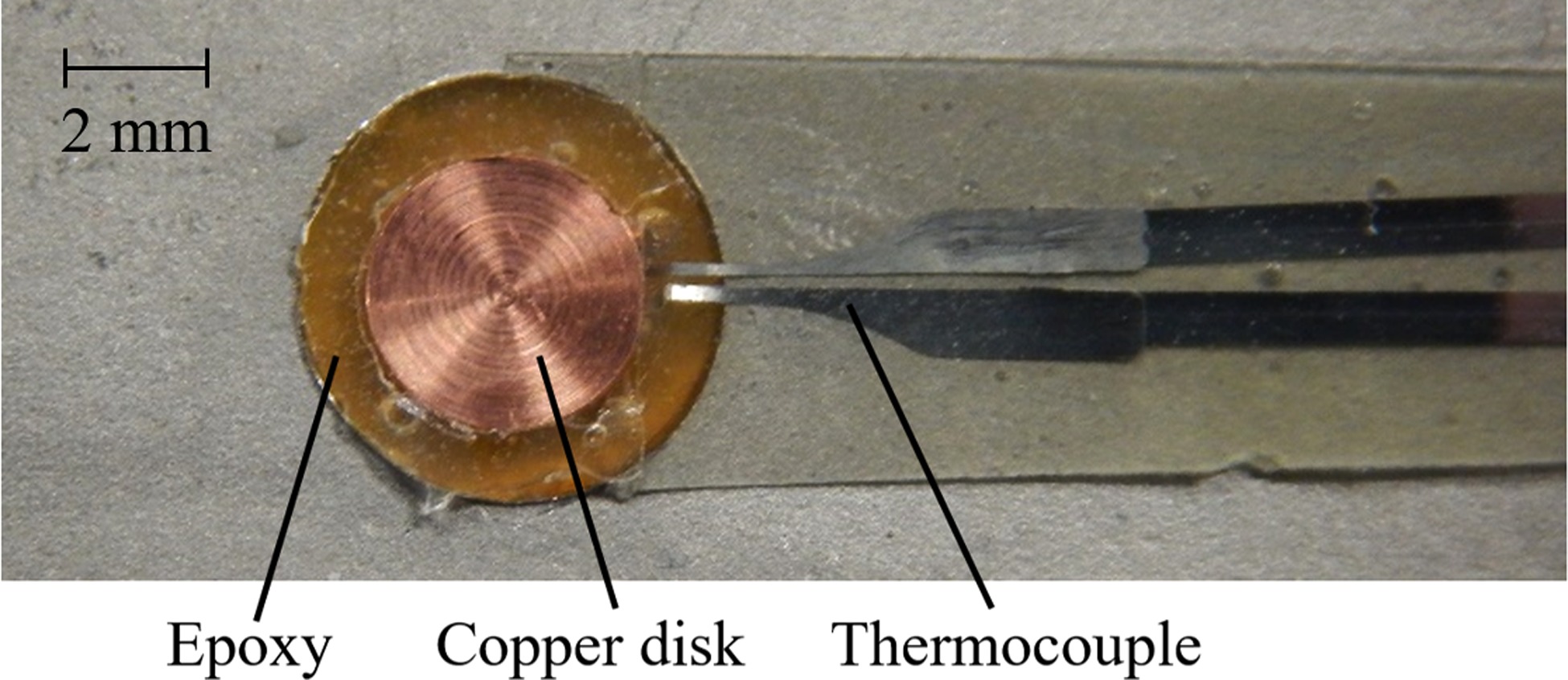
Table 3.
Properties of the elements in the assembly.
The proposed measurement system offers several advantages over conventional approaches, specifically:
the low thermal conductivity of the polyimide layer reduces the through-wall heat flux, and in combination with the copper layer, reduces the temperature difference between the thermocouple junction and external surface. This reduces the error between the thermocouple and the wall temperature directly above the thermocouple
we create a region in the IR camera field of view which is both larger and more isothermal than is typically provided on the target surface with a conventional application of the thermocouple, thus reducing errors associated with thermocouple localized in regions with high temperature variation (β2). In this arrangement the error between the thermocouple and the wall temperature local to but not directly above the thermocouple junction is no longer relevant, because we thermally isolate the calibration patch from the local environment.
the thermocouple junction is protected from the testing environment, allowing the measurement system to be used in high-speed flows.
Demonstration of the proposed measurement system
In this section, we demonstrate how the proposed measurement system (reference system 4) provides a large isothermal region in the FOV of the IR camera, while maintaining a low measurement error of type 1
To assess the errors in reference system 4, we created a one-dimensional steady-state heat transfer model of the system shown in Figure 9. The main source of error in the assembly of reference system 4 is the low thermal conductivity of the matt black paint layer applied over the copper disk, which has a range 0.500–1.50 W m−1 K−1 (Raghu and Philip, 2006). Figure 11 presents the contours of
Figure 11.
Analysis of reference system 4, showing difference between measured and true external surface temperature as a function of paint thickness and conductivity.
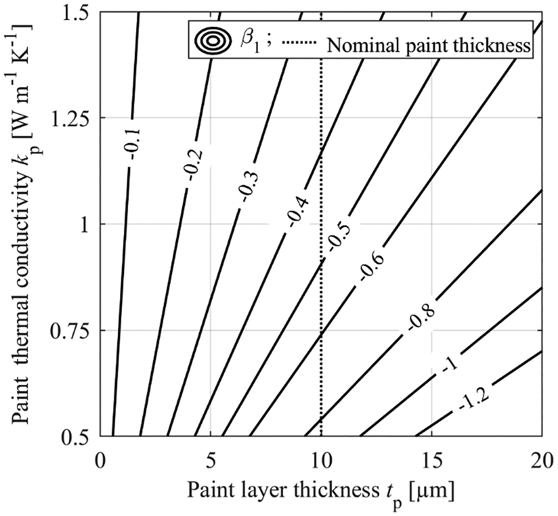
For a nominal paint layer thickness of 10.0 μm and the worst-case estimated value of paint thermal conductivity,
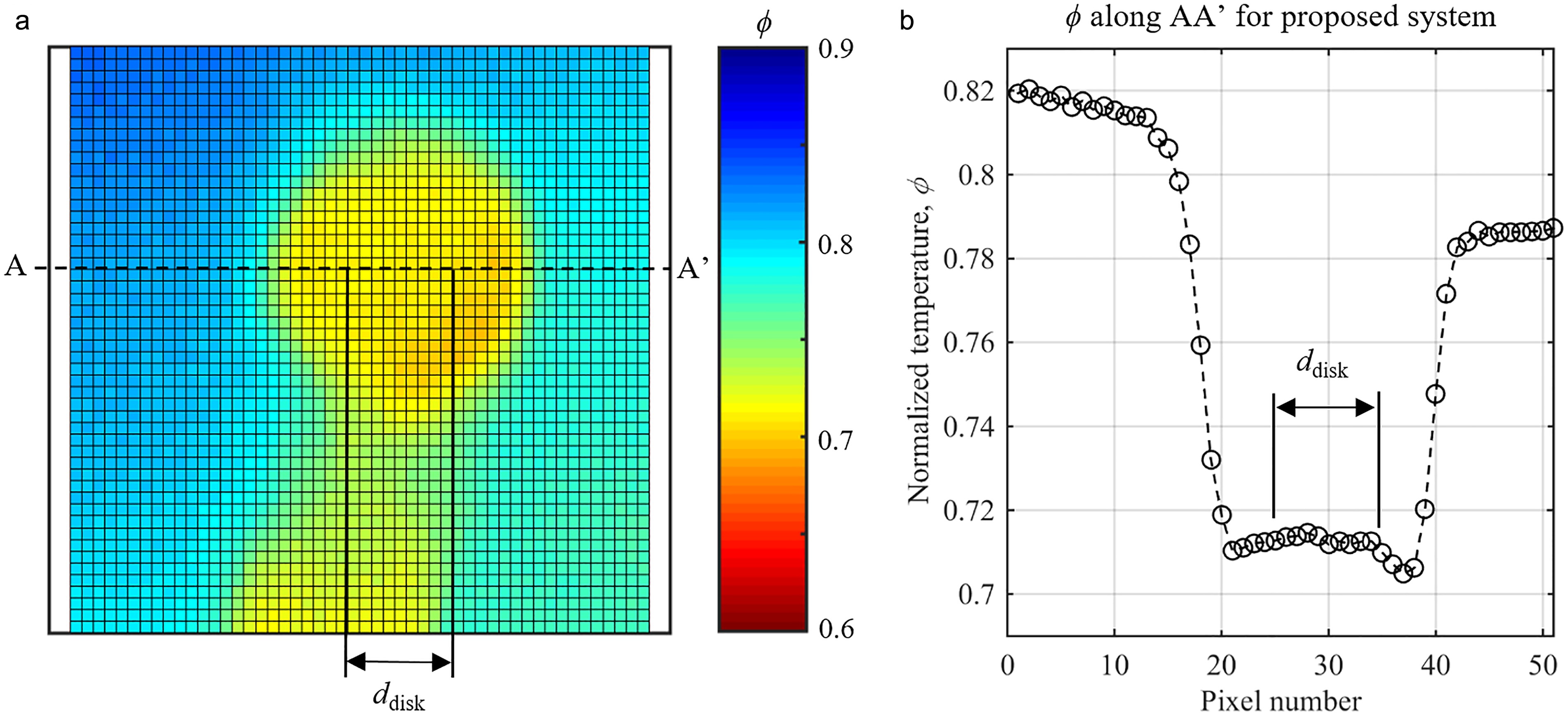
Figure 12 shows the experimental results from reference system 4 in terms of normalized temperature
Figure 12.
Proposed calibration system (reference system 4, see Figure 10): (a) surface plot of ϕ ϕ
Conclusions
In this paper, we present a systematic study of the sensitivity of two types of measurement errors (
Analysis of system 1 shows a wide range of
Analysis of system 2 shows that paint over the thermocouple increases
Analysis of system 3 show that an adhesive layer over the thermocouple leads to increased
Analysis of a proposed new system (system 4) shows that
The work of this paper is developed in response to the lack of data presented in the literature on the effect of typical calibration arrangements on the errors arising in in-situ IR calibrations in environments with high through-wall heat flux and lateral temperature gradient. It is hoped that this paper will present a framework for quantifying such errors in typical calibration arrangements, and that by adoption of the proposed technique error in the calibration process might be substantially reduced.