
Introduction
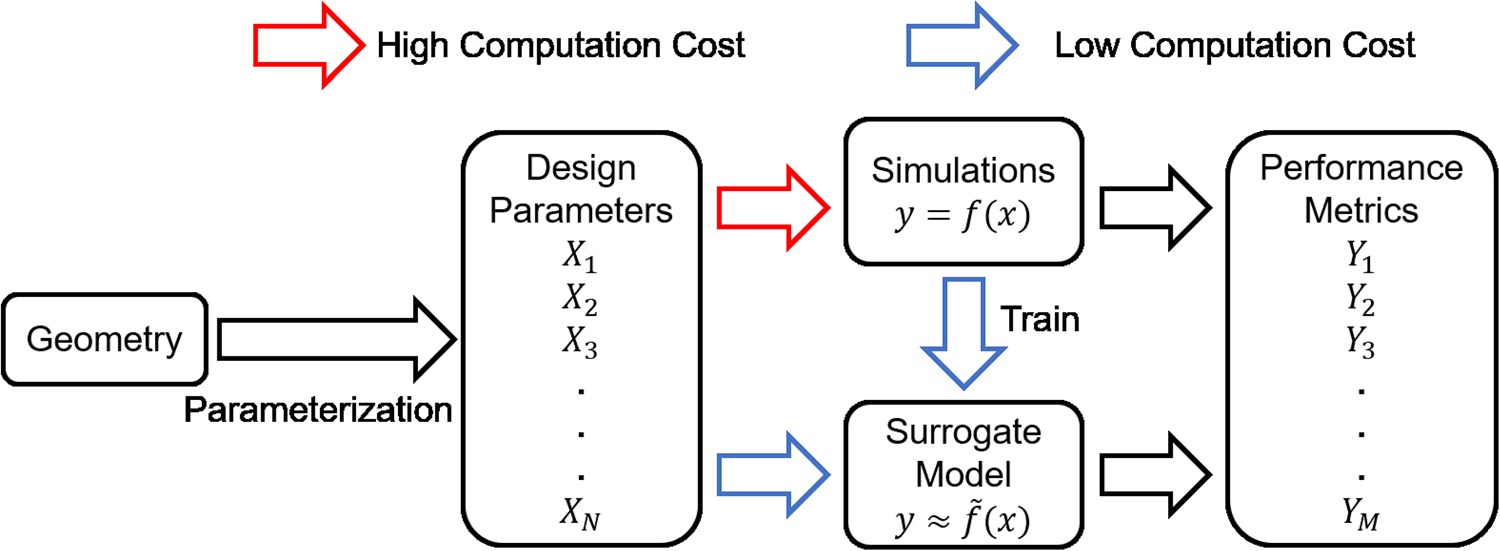
Surrogate model is widely used to accelerate the process of design and optimization of turbomachinery (Kipouros et al., 2007; Samad and Kim, 2008; Samad et al., 2008; Lee and Kim, 2009; Lee et al., 2014; Schnoes et al., 2018; Persico et al., 2019). It can predict the performance of new designs by utilizing previous results from numerical simulations or experiments rather than performing similar simulations or experiments repetitively. In the recent decades, a lot of surrogate model methods have been developed and applied in the industrial applications, for example, (1) Polynomial Response Surface Method (Myers et al., 2016; Hecker et al., 2017; Shuiguang et al., 2020); (2) Kriging Model (Sakata et al., 2003; Jung et al., 2021); (3) Radial Basis Function and Extended Radial Basis Function (Gutmann, 2001); (4)Artificial Neural Network (Mengistu and Ghaly, 2008); (5)Support Vector Machine (Lal and Datta, 2018). Figure 1 shows the process of existing surrogate model method, and one key step in this process is manual parameterization, which is to choose some important geometric parameters according to the experience of researchers to describe the geometry. In this step, if too few parameters were used, some geometric information will be lost because it is insufficient to describe geometries with high-order surfaces (e.g., airfoils and blades). On the other hand, using too many parameters or choosing irrelevant parameters will cause problems of over-fitting (Claeskens and Hjort, 2008). It is recognized that manual parameterization is the bottleneck that prevents further improvement of the performance of surrogate model method in terms of both accuracy and flexibility.
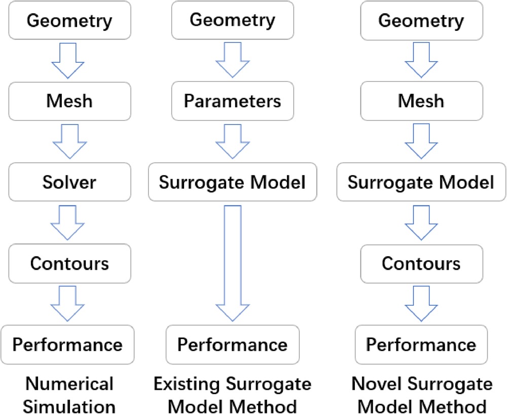
In this paper, a novel surrogate model method is presented, which establishes a mapping relationship between the surface meshes of fluid domain and two-dimensional distributions of fluid variables (in the form of contour maps) with Graph Neural Networks (GNNs), Convolution Neural Networks (CNNs) and a Conditional Variational Autoencoder (CVAE). Figure 2 shows the differences among numerical simulation used as analysis tools, the existing surrogate model method and the proposed novel surrogate model method. The new method can process the bounding surfaces of the fluid domain from the surface meshes used in the numerical simulations and extract relevant geometric features according to their significance to the result. Compared with the existing surrogate models, new method contains less uncertainties introduced by manual parameterization. This new method also allows different types of designs from different sources to be used because the geometry input to the model is the surface mesh, not user-defined parameters. In addition, the new method has the ability of predicting two-dimensional distributions of variables (in forms of contour maps) by utilizing CNNs to process the images.
Figure 2.
Comparison among numerical simulation, existing surrogate model method and novel surrogate method.
The ability of predicting two-dimensional distributions of variables is achieved by the application of CNNs. With the combination of convolutional layers, it can extract information from images, and recognize the convolutional result with multi-layer perceptron (Valueva et al., 2020). In this study, CNNs are used to predict the contours based on the latent distribution.
The ability of processing surface mesh is achieved by the application of GNNs. The nature of the graphic operation of GNNs make it capable to process the non-Euclidean domain by defining the connectivity of mesh points, while CNNs are only able to process regular Euclidean data like figures. Among existing GNNs variants (Scarselli et al., 2009), GNNs are categorized into three types: Recurrent GNNs, Spatial GNNs and Spectral GNNs. In this study, the surrogate model is built based on Spectral GNNs for its strengths in extracting features from meshes with large number of vertices (Wu et al., 2020). Spectral GNNs are built on signal processing theory. The key step, convolutional operation, is done by Chebyshev polynomial approximation (Hammond et al., 2011). In this study, GNNs are used to extract geometric information by optimizing parameters in the neural networks via back propagation of loss. This is to pick relevant information based on the feedback of prediction error, which avoids loss of geometric information and over-fitting problem. Also, the input of the new surrogate model can be both unstructured mesh and structural mesh thanks to the ability of GNNs to process non-Euclidean data.
Methodology
In this section, this non-parametric surrogate model method is introduced “top-down” by its architectural designs, namely, framework, blocks and then layers. Finally, the loss function used to train this surrogate model is demonstrated.
Framework of non-parametric surrogate model
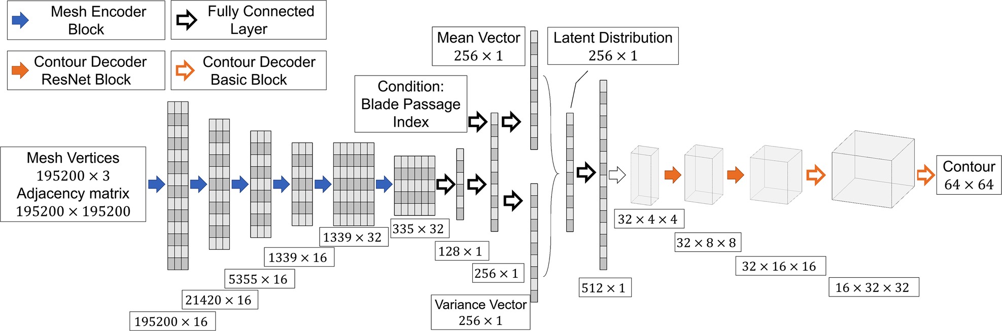
The framework of this new surrogate model method is shown in Figure 3. The mesh encoder block is a GNN encoder, which is to pick important geometric features from surface meshes. And the decoder block is a CNN decoder, which is to reconstruct the contours. Between the mesh encoder and contour decoder, there is a bottleneck that maps the extracted geometric information to latent flow variable distribution. The mapping relationship built through bottleneck needs much less training samples than directly mapping mesh vertices to contours because its input and output dimensions are much smaller. Also, it is easier to build a latent distribution for variational interface based on latent representation of geometric information in the bottleneck. The conditions in the model is blade passage index, which is to label different blade passages since the flow condition is asymmetric in the demonstration. In other applications, it can also be inlet boundary condition, material property and other important factors.
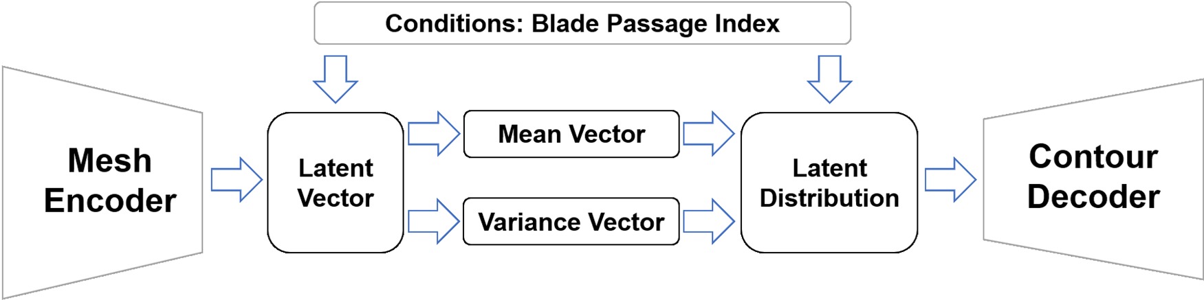
The structure of this surrogate model is basically a CVAE, which is an extension of AutoEncoder (AE). It is to compress graphical data to a latent vector and then reconstruct the graph with the latent vector. The neural network is trained to reconstruct the graphs with less error. Variational AutoEncoder (VAE) uses variational inference to estimate the latent vector rather than directly encoding from input graph (Blei et al., 2017). The latent vector z can be estimated by observation vector x using the following equation:
However,
Blocks in non-parametric surrogate model
The surrogate model presented in this paper contains two types of blocks: mesh encoder blocks and contour decoder blocks. The mesh encoder and contour decoder each consists of several blocks, the number of which depends on the size of mesh vertices and contour pixels. More mesh encoder blocks means a smaller latent vector, which contains less geometric information. But larger latent vector needs more training cases to prevent over-fitting.
Mesh encoder blocks
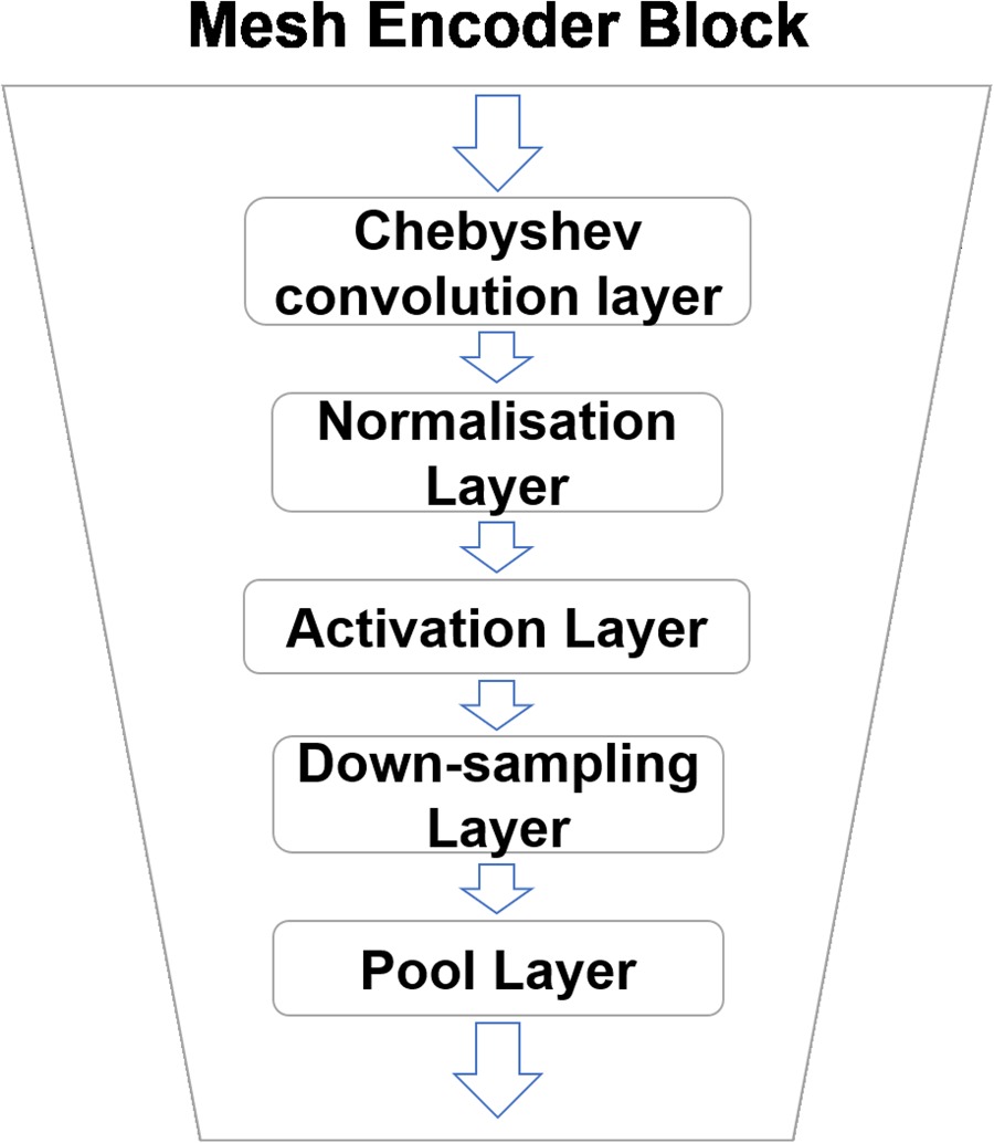
The structure of mesh encoder block is illustrated in Figure 4. One block has a Chebyshev convolution layer, a normalization layer (batch normalization), an activation layer (the rectified linear unit function), a down-sampling layer and a pooling layer (max pooling layer). The Chebyshev convolution layer is to scan the mesh vertices with Chebyshev polynomial filter and change the dimension of mesh vertices vectors. The normalization layer is to normalize the value of vectors in the same batch. And the activation layer is to zero the negative value in the vector. The down-sampling layer is to drop out irrelevant vertices based on the transformation matrix. The pooling layer is to keep the largest value and discard other values in the filter, which reduces the dimension of the vector. After several blocks, relevant geometric information is picked to form the latent vector. During a training process, the optimizer will optimize the parameters of each layer according to the loss function. In this way, the mesh encoder can keep important geometric information and discard insensitive information.
Contour decoder blocks
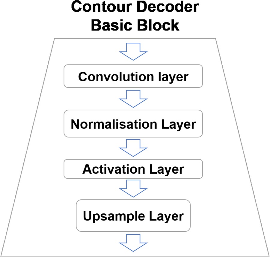
Contour decoder block is shown in Figure 5, which has four layers: a Chebyshev convolution layer, a normalization layer (batch normalization), an activation layer (the rectified linear unit function) and a upsampling layer. Convolution layer is to change the dimension of vector with convolutional filter. And then the vectors in the same batch are normalized by normalization layer. Activation layer is to zero the negative value in the vector. Upsample layer is to increase the number of elements in the vector. After several blocks, a latent distribution of large size is expanded to a contour of smaller size.
Two important layers in non-parametric surrogate model
Chebyshev convolution layer
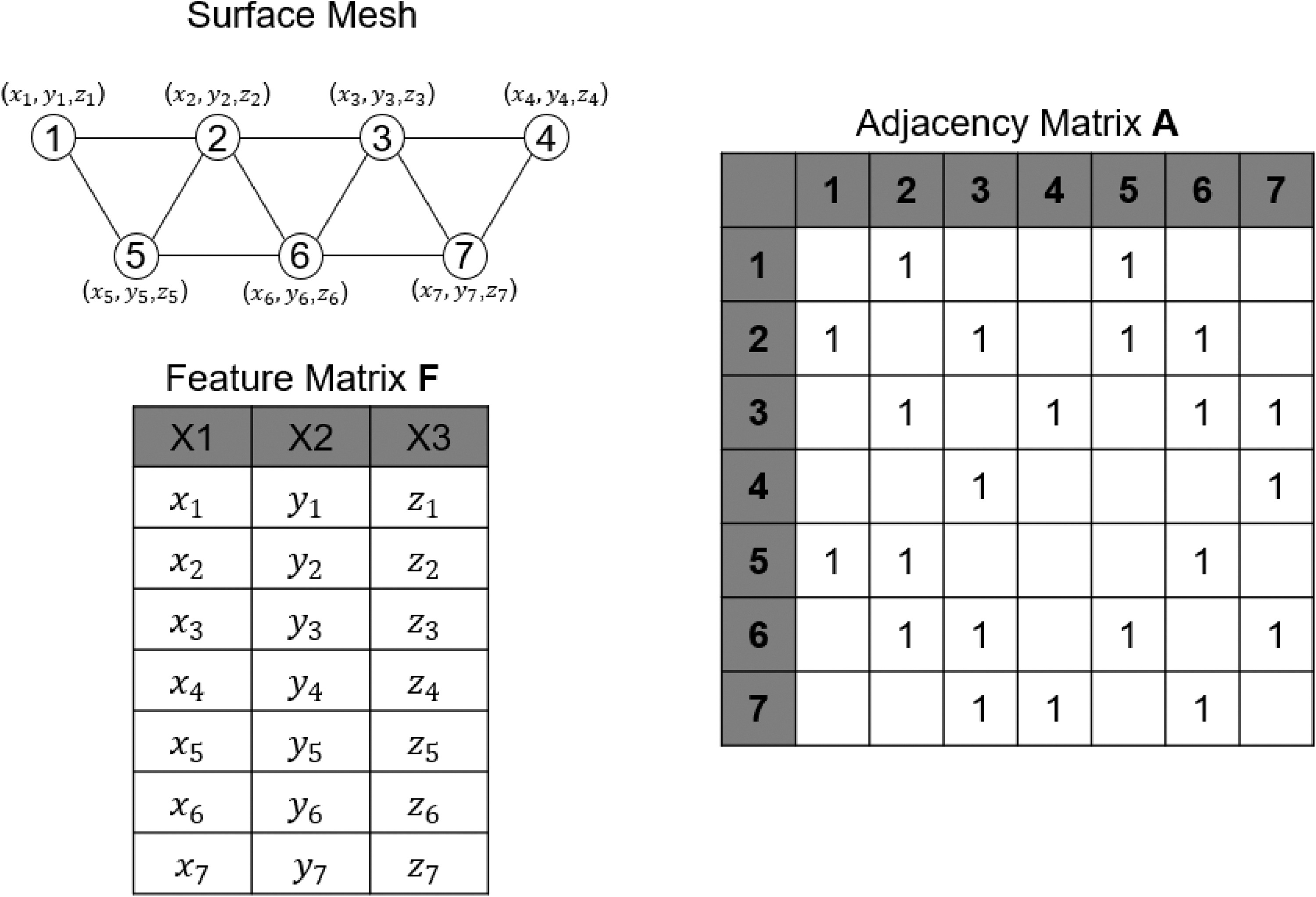
In this paper, as shown in Figure 6, the surface mesh M of the design is defined by the coordinates of vertices V and edges
The most important layers used in the mesh encoder is the fast spectral convolution layer, demonstrated in (Defferrard et al., 2016). The mesh convolution operator
To reduce the computational cost, convolution is conducted by a kernel
where
with the initial condition
With the mesh filter shown above, the fast spectral convolution layer can be expressed as the following equation with
where
Mesh sampling layer
Another important layer used in the mesh encoder is the mesh sampling layer, which includes the down-sampling layer and up-sampling layer in autoencoder (Ranjan et al., 2018). In the encoder, important information is chosen by down-sampling layer and irrelevant information will be discarded.
The convolution layers used in this study represents mesh in multi-scales so that mesh sampling layer can capture the local and global geometric information. The down-sampling operation is conducted by a transform matrix
Loss function
The loss function of the neural network consists of three types of losses: mean squared error (MSE) loss, Kullback-Leibler divergence (KLD) loss and structural similarity loss.
MSE measures the average of pixel-wise error between the contours predicted by model
KLD (Kullback and Leibler, 1951) measures the difference between one probability distribution and the reference probability distribution. In variational autoencoder, KL loss is the sum of all the KLD between the components in latent distribution and the standard normal distribution. With minimizing the KL loss, the latent distribution is closer to the standard normal, which can improve the interpolation and extrapolation ability of the surrogate model. KLD can be defined by:
(7)
As it is to measure the KLD between the components in latent distribution and the standard normal
where
Structural similarity loss measure, or SSIM (Wang et al., 2003), is a method to measure the similarity between two figures. Here, it is used to optimize the neural network to make predicted contours and simulated contours more structurally similar. It is defined by:
where
Finally, the loss function of the surrogate model is defined by the following equation:
where three coefficients
Demonstration of non-parametric surrogate model and application
In this section, the process of building a non-parametric surrogate model for LPES is introduced in details.
Introduction of low-pressure steam turbine exhaust system
LPES is designed to maximize the recovery of the kinetic energy leaving the low-pressure steam turbine and convert it to static pressure rise for the condenser. It usually consists of three parts: an axial-to-radial diffuser, an asymmetric collector, and an extension.
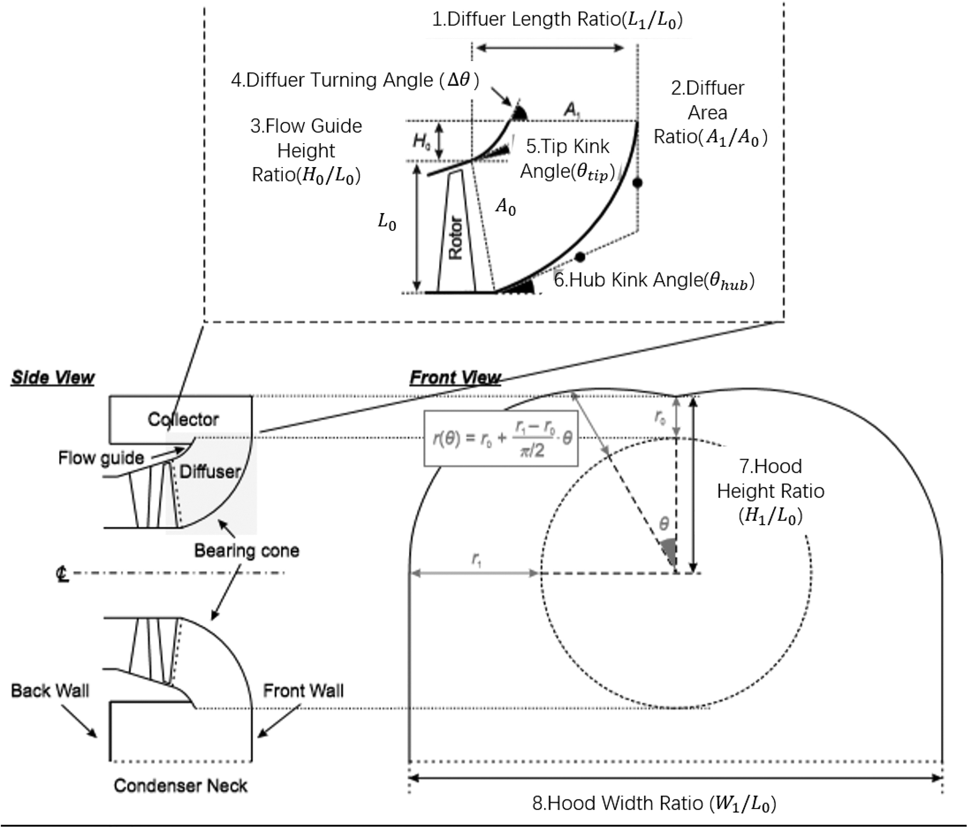
It is quite challenging to build surrogate model for LPES with the existing surrogate model methods because parameterization of geometry is problematic. Figure 7 shows a parameterization method to define the geometry of the system from (Ding, 2019), namely, the diffuser length ratio
Figure 7.
A typical down-flow type low-pressure exhaust system for large steam turbine. Figure adapted from (Ding, 2019).
In this surrogate model, there are two sets of LPES geometries defined by different parameterization methods. One is defined by 95 parameters, the other one by 66 parameters. The first one firstly defines the cross-section of diffuser and collector, and then revolves it with an ellipse equation to generate circumferential distribution. It also has asymmetric features in extension. The second one directly defines the cross-section along the axial direction with ellipse equations. Two genetic-based optimiztion systems with these two sets of parameters are used to accumulating dataset for surrogate model. With two types of geometries, the ability of processing geometries from different sources can be tested.
Mesh generation
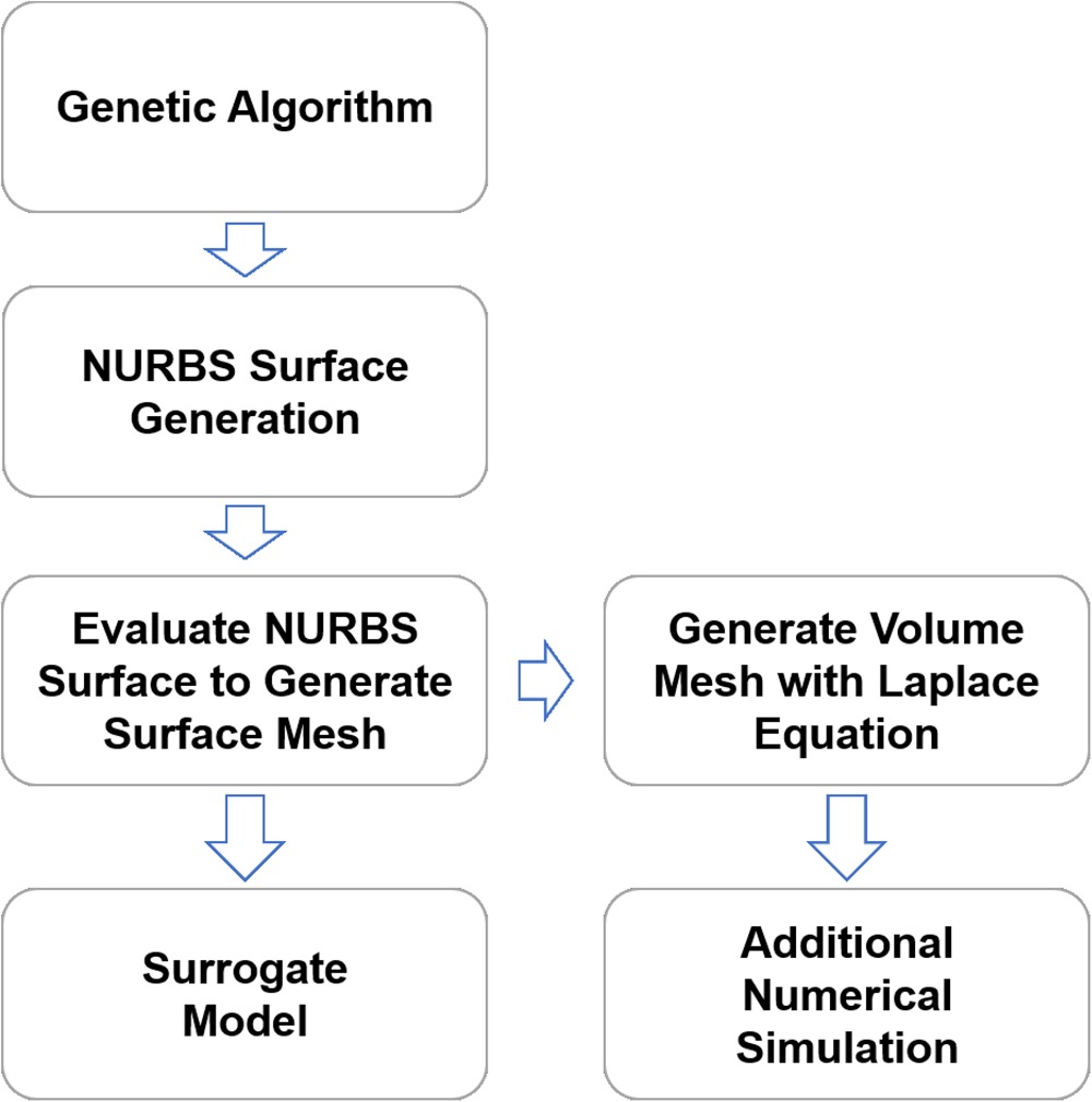
The mesh generation process is shown in Figure 8. It starts from the coordinates of control points given by genetic algorithm. The control points are used to generate Non-Uniform Rational B-Spline (NURBS) surfaces, and then evaluate the NURBS surfaces to generate the surface mesh. These surface meshes, shown in Figure 9 are the input of surrogate model. Volume meshes are generated with the elliptic mesh generation method similar to (Spekreijse, 1995), which is by solving Laplace equation:
The boundary condition is defined by the coordinates of surface mesh. Since the Laplace equation represents a potential field, equipotential lines do not intersect and are orthogonal at vertices. The volume mesh can be generated by solving x, y, and z coordinates potential field respectively. And the refinement of mesh can be done by refining the surface mesh, and then the volume mesh is also refined because surface mesh is the boundary condition of Laplace equation. The surface mesh can be refined by re-evaluating the NURBS surface with different distribution functions. This mesh generation method is also able to generate meshes for the fluid domain with the same topology, regardless changes in geometry.
Numerical simulation setup
Simulation domain
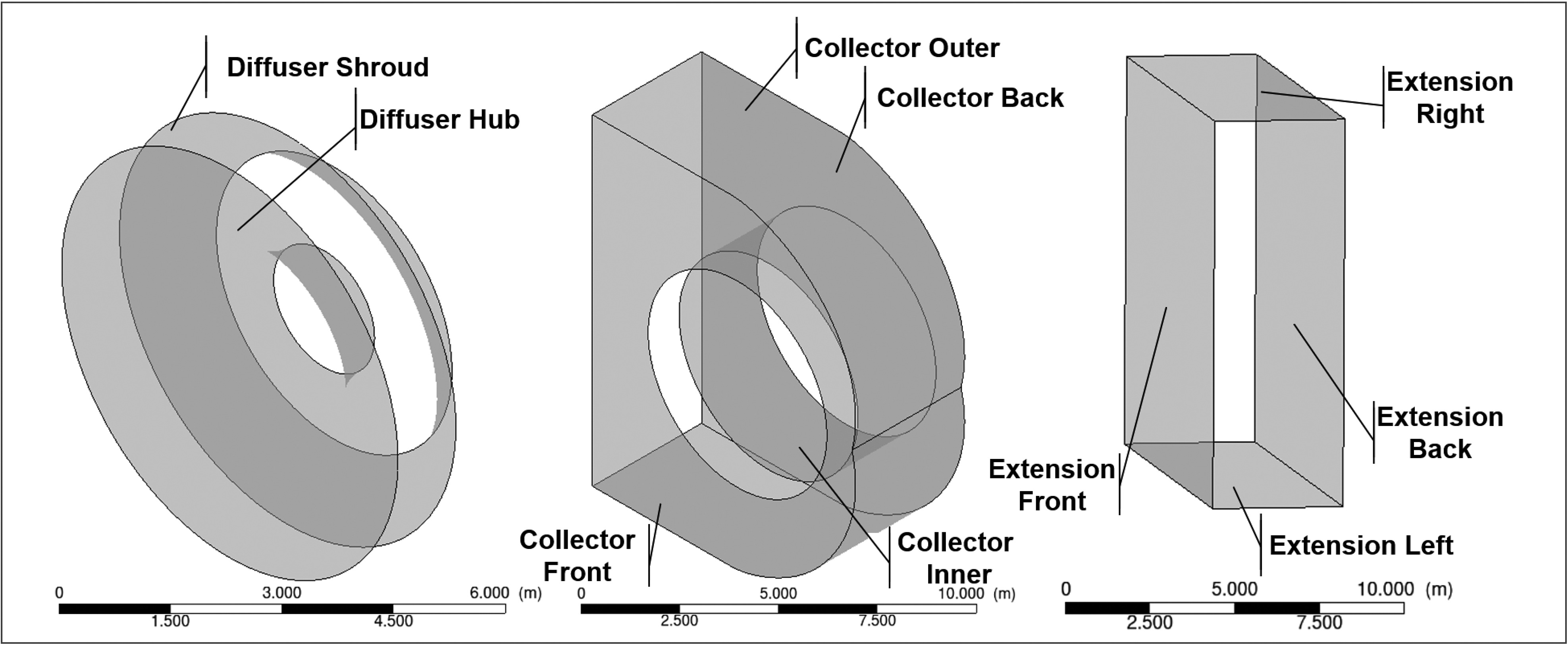
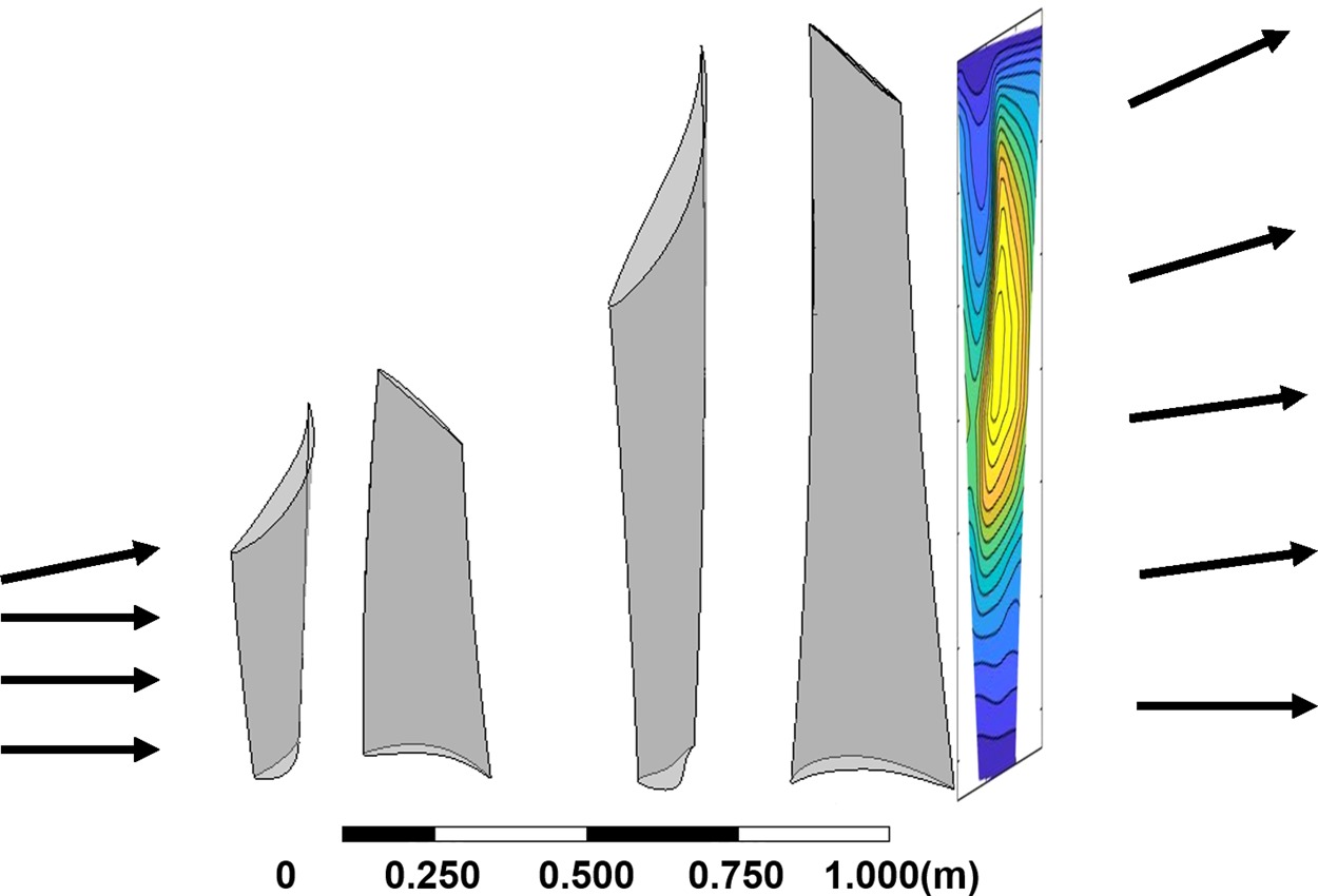
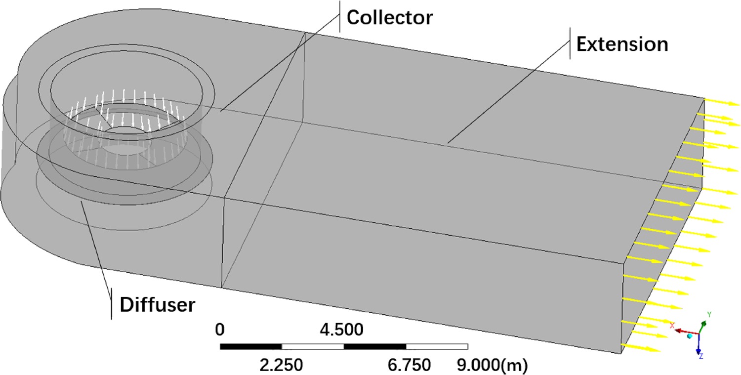
The fluid domain of numerical simulations includes: the last two stages of low-pressure steam turbine, an axis-asymmetric axial-to-radial diffuser, a collector and an extension. Figure 10 shows the geometry of two turbine stages, which represents the last two stages of a typical large steam turbine. It can generate a representative inlet boundary condition for the exhaust system. Figure 11 shows the geometry of the axial-to-radial diffuser, collector and extension in the downstream. The stage-hood interface treatment method is multiple mixing plane method with four blade passages. Each of them generates inlet boundary condition for a 90-degree diffuser section (Ding, 2019).
Simulation setup
The solver used for the numerical simulations is Ansys CFX, which is a widely-used commercial CFD solver for the research community and industry. The simulation is a Reynolds-averaged Navier–Stokes (RANS) simulation, which uses
The inlet boundary condition is applied at the inlet of the simulation domain, which has total pressure and total enthalpy. The flow direction at the inlet is normal to boundary. And the outlet of the simulation domain is at the end of extension, which is applied with static pressure boundary conditions. The flow direction at the outlet is also normal to boundary. To perform the part-load simulations, the total pressure is reduced at the inlet to reduce the mass flow rate and work output. The static pressure at the outlet is 6.2 kPa according to the steam property at the condenser. For the property of the working fluid, steam, IAWPS data has been used, which is embedded in CFX and also widely used in the research community and industry.
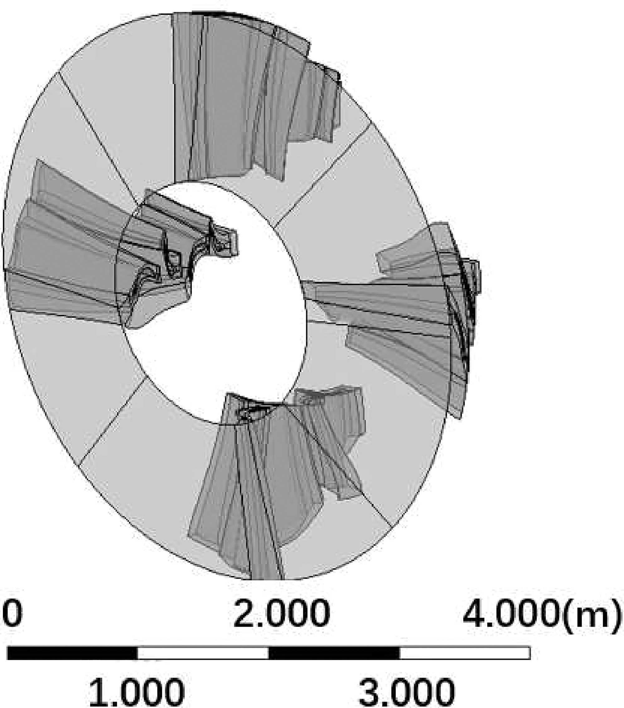
Another setup worth mentioning is the interface treatment method between stages and the inlet of the diffuser. Because the downstream of the diffuser are asymmetric, it is necessary to model the circumferential non-uniformity. The multiple mixing plane method (Burton et al., 2013) is used in this study. Figure 12 shows only four-blade passages are simulated to generate inlet flow conditions for the low-pressure exhaust hood, which means the outlet boundary condition of one blade passage are copied to cover a 90-degree section of the diffuser. Multiple mixing plane method, though losing accuracy with only 4 blade passages, can reduce the computational cost considerably.
Processing of numerical simulation results
The objective of GA-based optimization is to increase power output of the last two low pressure steam turbine stages. It is calculated by the difference between the total energy fluxes pass through inlet and outlet of the last two stages, which is summed value of all the elements of contour map of energy flux. Assuming the system is adiabatic, the power of each element is obtained by the product of local total enthalpy and local mass flow rate:
Since the inlet boundary condition is known in the simulation, only the total enthalpy contours and mass flow rate contours at the outlet of the last two stages are extracted from numerical simulations to generate power contours as shown in Equation 12, which will also be the output of the surrogate model. Because of the multiple mixing plane method, there are four blade passages for each simulation, and five workload conditions for each design. Admittedly, there is certainly some uncertainties in the numerical simulations, but it is not primary concern in this paper since the key of this study is to develop a new surrogate model method.
Neural network setup
The neural network is built under the framework of Pytorch. Figure 3 shows the main structure of network. Figure 13 shows the change of feature dimension through the network. The input is 10 bounding surface meshes of fluid domain, which have 195,200 vertices in total. All the samples need to be interpolated to the same number of mesh vertices to represent the geometry at the same details level. Therefore, the input data is the coordinates of vertices
Test result
In this demonstration, 550 cases are used for training, and the test dataset has 32 cases. Each case contains total enthalpy flux distribution contours for 4 blade passages at 5 workload conditions (640 contours in total).
Figure 14 is to demonstrate the ability of predicting contours and capturing flow features. It shows some representative contours of the test cases, which presents some typical flow features of 5 workload conditions. Most flow features are predicted well in Figure 14, which provides more information than existing surrogate model methods. For example, the separations in the near hub regions are well captured in the contours of 50% workload condition. And the vortices are also well predicted in the contours of 70% workload condition. These information can tell users the reason of performance improvement during the optimization process rather than only several performance metrics.
Figure 14.
Contour results of numerical simulation and machine learning of some typical flow features at five workload conditions. (50 % 60 % 70 % 85 % 100 % 1 × 10 4 kJ / s
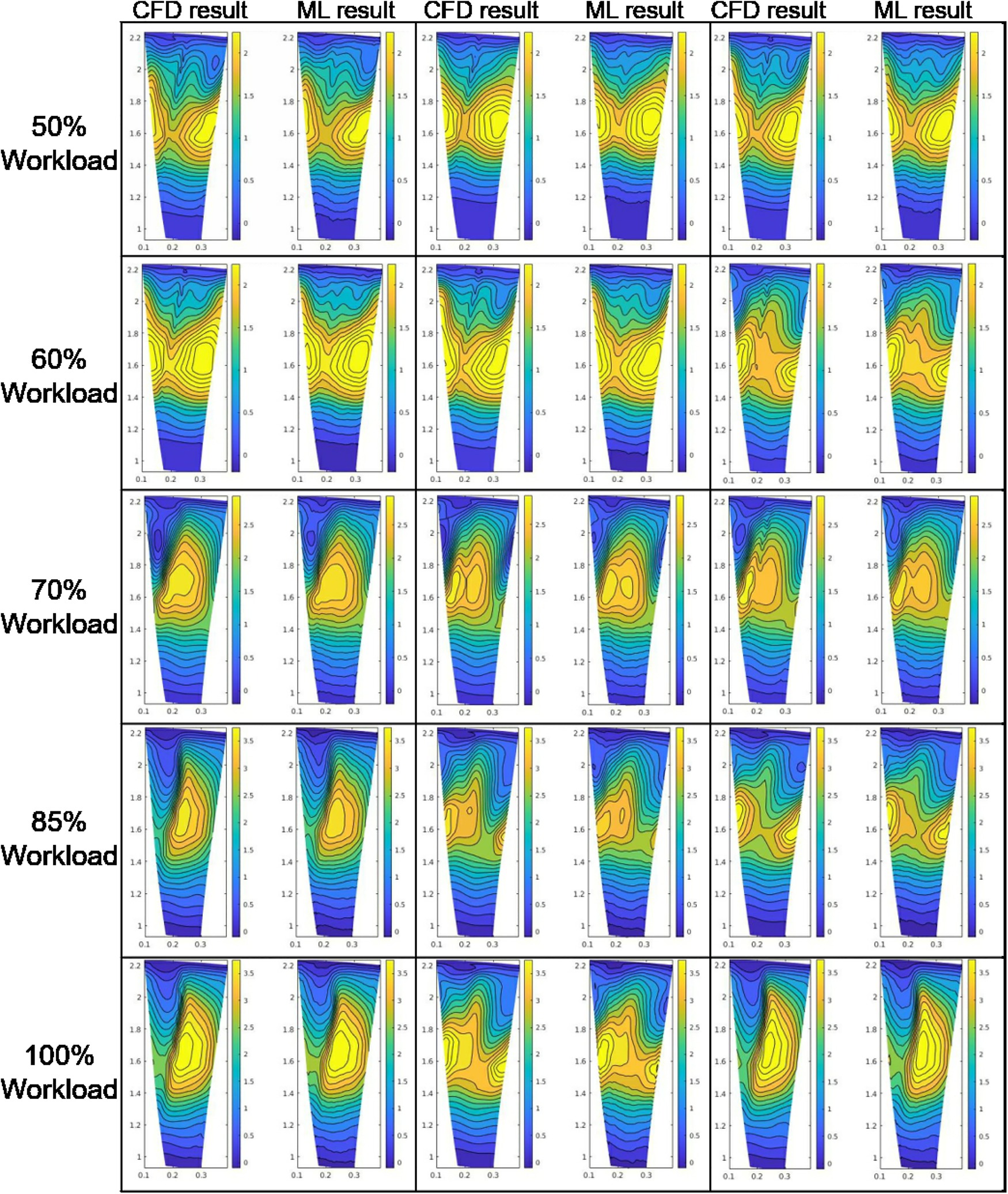
Table 1 summarizes the results of all 640 test contours. The averaged summed value error of dataset is 0.86%, which is able to screen suitable designs and accelerate the optimization process. The last few optimization iterations may still rely on numerical simulation. Also, test dataset is consist of two sub-datasets that contain geometries defined by two parameterization methods, both of which have 16 cases and 320 contours. In Table 1, The similarity measure of sub-dataset1 and sub-dataset2 are 0.9580 and 0.9609 respectively, which has no significant difference. This proves the generalization capability of the proposed method in processing geometries defined by different parameterization methods.
Table 1.
Summary of result. Sub-dataset1 are geometries defined by 95 parameters and sub-dataset2 are defined by 66 parameters.
Figure 15 plots the predicted performance against results from numerical simulations. Most of points are close to

Discussion
The new surrogate model method established a mapping relationship between the surface mesh of fluid domain and two-dimensional distribution of flow variables. Using GNNs to extract geometric information, the application of this new method can be extended beyond the area of aerodynamics optimization. Thanks to its ability of processing both structured and unstructured mesh, it is also applicable in various problems in different fields, which are solutions of partial differential equations, traditionally using finite element analysis and electromagnetic analysis methods.
This method can also be used as an inverse design method. It can be achieved by exchanging the input and output of the mapping relationship built in this paper. To be more specific, users can import the desired two-dimensional distributions of physical properties into the contour encoder, and the designs could be created by the mesh decoder.
In the application scenarios, one common problem of surrogate model method is users do not know whether they can trust the result of surrogate model or not. If the new design is quite different from designs in the training dataset, it is better to perform numerical simulations. To tackle this problem, the new method can identify the new design by calculating the KLD of their latent vectors. Higher KLD usually means the new design needs numerical simulation to evaluate its performance.
Conclusion
This study demonstrated a novel non-parametric surrogate model method with application on LPES design and optimization. The new method directly takes surface mesh as the input, which reduces the uncertainties introduced by manual parameterization and loss of geometric information. This feature gives the method greater advantages in building surrogate model for designs with complex geometries. In the test, the average summed value error of 640 contours is 0.86%.
This method also shows high flexibility and compatibility. Because the input of this method is surface mesh of simulation domain, it can take geometries of the same topology as its database. This means it can process geometries defined by different parameterization methods. This feature is very useful for further increasing the size of database of surrogate model using variable sources of data.
Compared with existing surrogate model methods, this new method can also predict two-dimensional distribution of variables (contour maps) based on surface mesh. Contours can help designers to identify physical mechanism, improve designs and for many other purposes. In the test, the average similarity score of 640 contours is 0.9594, which indicates that most of the pertinent flow features have been captured.
The essence of this method is the establishment of a mapping relationship between the surface mesh of the simulation domain and distributions of physical variables on certain two dimensional cut planes. With this method, the optimization process of an engineering system with complex geometry features such as LPES could be accelerated by utilizing the database created by various means to evaluate the performance of new designs.