Introduction

The defining feature of highly transonic turbine stators is the considerable difference between the blade metal angle and the actual flow angle downstream of the trailing edge, namely, the flow deviation. Accurately predicting the flow deviation is particularly relevant during the preliminary design of axial turbines, as small errors can turn into large variations of specific work, power output and efficiency (Osnaghi, 2002).

Several models for estimating the magnitude of the flow deviation are available in literature. Among these, correlations by Traupel (2019) and Ainley and Mathieson (1951) are still widely used to preliminary estimate the deviation during the turbine meanline design. However, although such correlations have been thoroughly assessed for conventional turbine applications using air or steam as working fluids, no analysis has been performed on turbines operating with fluids in the dense vapor thermodynamic state yet. Such machinery is used, for example, in organic Rankine cycle power systems (Colonna et al., 2015). In the thermodynamic cycle, a dense organic vapor (e.g., fluorocarbon, hydrocarbon or siloxane) is expanded in a turbine starting from a thermodynamic inlet state clofse to that of the critical point. These turbines operate with comparatively higher expansion ratios than those characterizing conventional ones. Moreover, the flow is highly transonic/supersonic, arguably leading to significant flow deviations downstream of the stator vane.

Studying the influence of both the non-ideality associated to the dense vapor state and the molecular complexity of the working fluid on the internal flow field is thus paramount to correctly design turbine cascades and accurately predict the flow deviation. The non-ideal fluid dynamics of dense vapor flows is governed by the so-called fundamental derivative of gas dynamics (Thompson, 1971), defined as

(1)
Γ1+ρc(cρ)s=12[γpv+1vγpv(γpvv)s],

where ρ is the density, c the speed of sound, and s the entropy. Equation 1 also introduces the generalized isentropic pressure-volume exponent (Kouremenos and Antonopoulos, 1987), defined as

(2)
γpv=vp(pv)s=vpcpcv(pv)T=γβTp,

where γ is the ratio of the specific heats and βT is the fluid isothermal compressibility. In the dilute gas state, γpvγ and Γ(γ+1)/2, where γ is the ratio of specific heats. Conversely, if the fluid is in the dense vapor state, the γpv value varies over the expansion. As a consequence, the internal flow pattern substantially departs from the one which can be encountered in machines operating with fluids such as steam or air. For example, expansions in convergent-divergent nozzle cascades from supercritical inlet thermodynamic states can exhibit strong non-ideal effects which determine a different shock and expansion pattern from that characterizing ideal gas processes (Romei et al., 2020). Previous works (Giuffré and Pini, 2021; Tosto et al., 2021) pointed out that the average value of γpv over an expansion can be used to measure the influence of non-ideal flow effects on the turbine performance and operation. In particular, compressibility effects in turbomachinery blade rows operating in the non-ideal compressible flow regime can be greatly enhanced or mitigated depending on whether the generalized isentropic exponent γpv is higher or lower than the heat capacity ratio γ of the fluid in the limit of dilute gas (Baumgärtner et al., 2020; Romei et al., 2020). Furthermore, if evaluated under the limit v, both Γ and γpv show a monotonic decreasing trend with the molecular complexity of the fluid (Tosto et al., 2021). In addition, thermodynamic dense vapor states of organic compounds, such as the ones used in ORC power systems, are characterized by values of Γ and γpv which are significantly lower than those characterizing the dilute gas state. Therefore, it is expected that non-ideal flow effects significantly affect the flow deviation downstream of the cascade.

Non-ideal effects also influence the turbine loss breakdown which, in turn, affects also the design of the cascade. Indeed, the presence of strong gradients of thermo-physical properties, together with flow compressibility, affects the dissipation produced by various loss mechanisms, such as those associated to viscous effects in boundary layers, shocks, and mixing at the blade trailing edge. Eventually, this results in optimal designs which are significantly different from those that would be obtained through the application of existing best practices (Wilson, 1987; Giuffré and Pini, 2021).

An additional problem that may arise in ORC turbines is the onset of critical choking conditions, which is intimately connected to the flow deviation. Critical chocking occurs when the meridional Mach number at the cascade outlet reaches unity. This condition differs form the turbine choking conditions, which, in turn, arises when the Mach number in the passage throat reaches unity. When a turbine vane is in critical choking conditions, both its operability and efficiency are severely compromised. Therefore, the design of ORC turbines has to be carried out to avoid critical choking in both design and off-design conditions. Furthermore, in mini-ORC turbines, the expansion ratio is so high that the flow is strongly supersonic and the machine might meet critical choking at partial load (De Servi et al., 2019).

This paper presents a study on the effects of fluid molecular complexity and thermodynamic non ideality on both flow deviation and critical choking. The analysis is first addressed from a conceptual standpoint by resorting to theoretical models. Then, Reynolds Averaged Navier-Stokes (RANS) simulations are performed to obtain quantitative information on the value of flow deviation in a representative transonic ORC turbine vane. Results are compared against trends obtained by reduced-order physical models (ROM) that can be used for design purposes. Finally, a loss breakdown analysis is performed to gain further insights on the mechanisms of dissipation in the boundary layer and in the mixing region and their relation with flow deviation. The paper is structured as follows. Section 2 introduces the concept of corrected mass flow per unit area in swirling flows of dense vapors. Qualitative findings regarding the deviation downstream of a transonic turbine cascade, as well as the role of the isentropic exponent γpv on the flow expansion, are discussed. Section 3 reports the methodology and the results of the numerical assessment conducted on a representative transonic turbine cascade. The trends of both flow deviation (Sec. 3.2) and irreversible entropy generation (Sec. 3.3) with flow compressibility, fluid molecular complexity and thermodynamic non-ideality are discussed. Insights on the physical mechanisms explaining such trends are also provided. The accuracy of the reduced order models is then evaluated against the numerical results. Finally, the main outcomes of this work are summarized in Section 4.

Theoretical background

The corrected flow per unit area, which is a direct measure of the flow capacity of the stage (Greitzer et al., 2004), allows one to conceptually understand the influence of flow deviation on performance of turbine cascades. This quantity is also particularly useful to examine choking regimes.

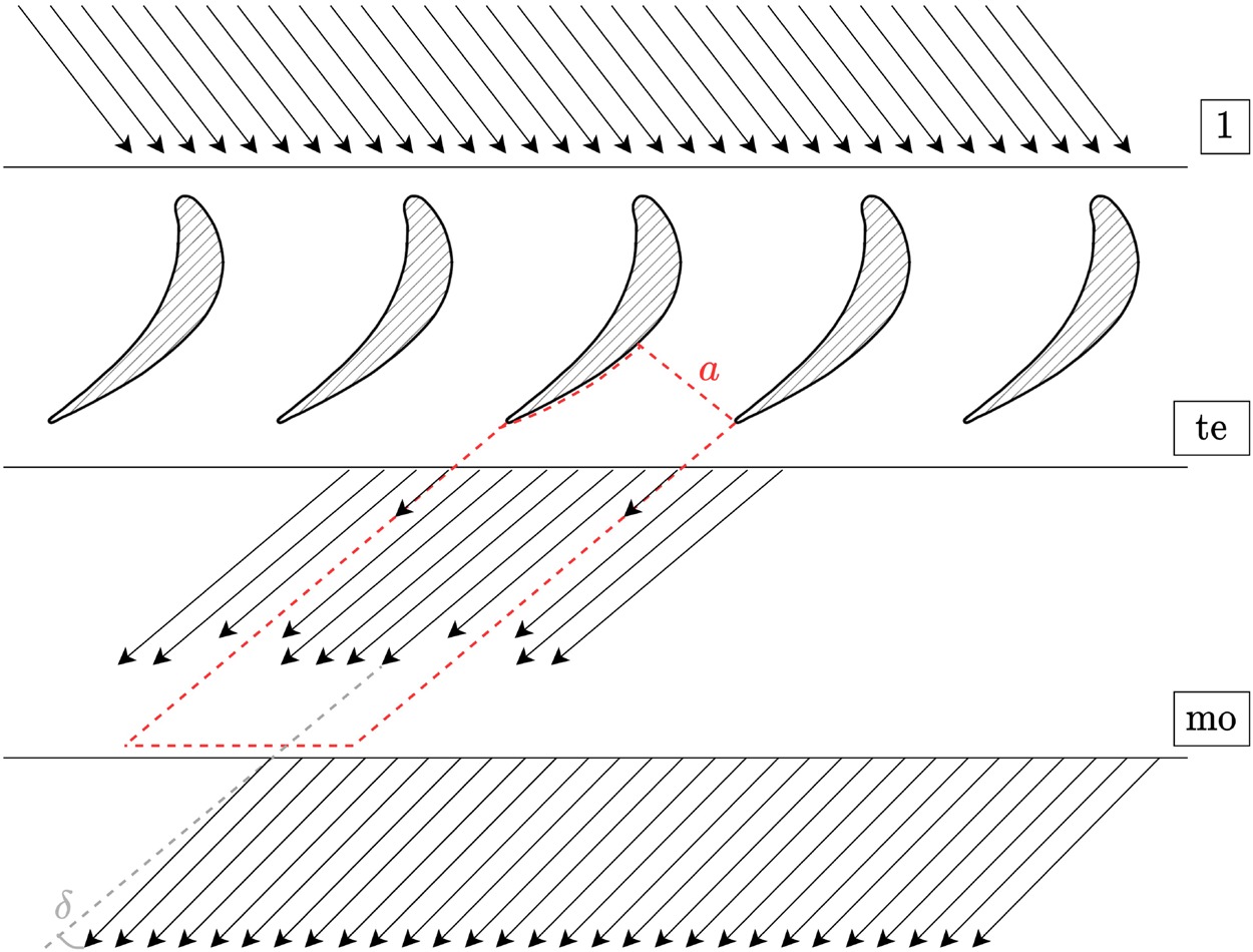
The expression of the corrected mass flow per unit area for ideal gas flows can be rearranged to highlight the role of the swirl velocity component. With reference to Figure 1, the corrected flow per unit area reads

Figure 1.

Axisymmetric swirling flow in a duct with velocity components.

https://journal.gpps.global/f/fulltexts/151659/JGPPS-00129-2022-02.01_min.jpg
(3)
m˙corr=m˙RTtptAγ=TTtρρtVmγRTt=Mmf(M),

where Mm is the meridional Mach number, and

(4)
f(M)=(1+γ12M2)((γ+1)/2(γ1)).

We are here neglecting the swirl component in the radial direction, i.e., ϕ=0 in Figure 1.

Using the relations proposed by Baltadjiev (2012), Equation 3 can be generalized to an arbitrary fluid in whichever state by making use of the isentropic exponent γpv. If the fluid state is sufficiently far from the critical point, the partial derivative in Equation 1 can be neglected, and an analytical relation between γpv and Γ holds. Such approximation has been exploited, for example, in some experimental and numerical works on turbine cascades for ORC power systems (Wheeler and Ong, 2013; Baumgärtner et al., 2020). The general definition of the corrected mass flow is thus given by

(5)
m˙corr=m˙ZtRTtptAγpv=Mm(1+((γpv1)/2)M2)((γpv+1)/(2(γpv1))),

where Zt=pt/(ρtRTt) is the flow compressibility factor defined at total conditions. Further algebraic manipulation leads to

(6)
m˙corrm˙ρtctA=(1+γpv12M2)M21+((γpv1)/2)M2(Vθγpv,tZtRTt)2,

where the second term under the square root is the so-called swirling parameter and denotes the amount of swirl of a given flow. Equation 6 shows the relation between the corrected flow per unit area and the swirling parameter. Using the isentropic relation pt/p=f(M,γpv), which is valid regardless of the thermodynamic state of the fluid (Baltadjiev et al., 2015), Equation 5 can also be rewritten in terms of both pressure ratio and flow (swirl) angle, namely

(7)
m˙corr=(ptp)((γpv+1)/2γpv)2γpv1[(ppt)((1γpv)/γpv)1]cosα.

Note that the accuracy of the results obtained by applying the above equations depends on the actual variation of γpv along an expansion process and is therefore related to the extent of the flow non-ideality, namely on the relative difference between γ and γpv, and to the flow Mach number.

Equations 6 and 7 allow us to investigate the influence of the working fluid and the operating thermodynamic state on the swirling flow developing in turbine cascades. The entity of the deviation of the γpv value from that of the specific heats ratio γ is used to measure the fluid non-ideality. Figure 2 shows the contours of γpv for two fluids at different level of complexity of their fluid molecules, namely siloxane MM and CO2. These processes highlight that flow expansions in such machinery exhibit γpv values that not only non-monotonically vary over the process, but can also be significantly lower than the γ value of the fluid computed in the dilute gas state.

Figure 2.

Thermodynamic temperature-entropy diagrams of CO2 (a) and siloxane MM (b). Pressure and γpv contours are reported. γpv values have been calculated using the relation γpv=γ/(βTp) (see Equation 1), where βT has been estimated resorting to a well-known database of fluid properties (Lemmon et al., 2018). CP and VLE denote critical point and saturation vapor-liquid curve. Figure 2b also shows the expansion processes of cases iMM and niMM, which are discussed in Sec. 3.

https://journal.gpps.global/f/fulltexts/151659/JGPPS-00129-2022-02.02_min.jpg

Table 1 lists the main properties of the fluids investigated in this work, together with the maximum and minimum values of γpv occurring in the thermodynamic region bounded by p<2.5pcr and s>scr. Note that the higher the molecular complexity, the lower the γpv value that the fluid exhibits in the considered thermodynamic region (Tosto et al., 2021).

Table 1.

Characteristic fluid properties of air, carbon dioxide and siloxane MM. γ is the specific heat ratio calculated in the dilute gas state. The lower and upper bound of γpv are those occurring in the thermodynamic region defined by s>1.01scr and by the thermal stability limits of each molecule.

Mmol [kg/kmol]Tcr [K]pcr [bar]γγpv,minγpv,maxΓ
Air28.96132.8238.501.401.442.851.20
CO244.01304.1373.771.290.864.331.13
cyclo-pentane70.13511.7245.711.060.574.111.03
MM162.3518.7019.311.030.394.751.01

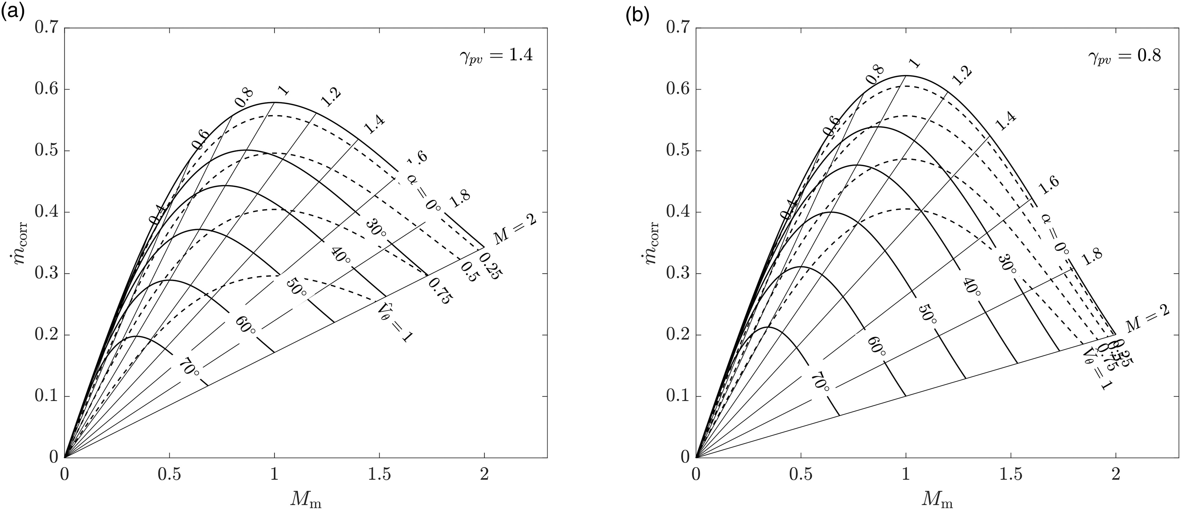
Figure 3 shows the trend of corrected flow per unit area as a function of the meridional Mach number Mm for two values of generalized isentropic exponent γpv. The first γpv value is representative of a dilute bi-atomic gas such as air, while the second one is representative of a dense organic vapor. In the charts, lines of constant absolute Mach number M, swirl angle α, and swirl parameter V^θ=Vθ/γpv,tZtRTt are also displayed. The graphs show that the vertical line corresponding to Mm=1 passes through the maxima of the curves at constant u^θ. This means that critical choking in swirling flows is reached when the magnitude of the meridional velocity component equals that of the speed of sound and the flow is already in the supersonic regime, i.e., M>1. The value of total Mach number at which choking occurs strongly depends on the γpv value. For instance, by assuming V^θ=0.75, critical choking is achieved at M1.2 for γpv=0.8 and at M1.4 for γpv=1.4. This finding has important consequences on both the design and operation of a turbine. Given that the line at Mm=1 represents the physical limit of operation of a turbine (Mm>1 would entail the impossibility of the flow to adapt to outlet conditions), it is common practice to design swirling devices in the transonic/supersonic regime with sufficient margin from that limit. If the working fluid is in a condition such that γpv<γ over the expansion process, the condition Mm=1 would be reached at a lower value of absolute Mach number, and thus the turbine vane cannot be designed for highly supersonic flows. Conversely, if the working fluid is in a condition such that γpv>γ, no such problem exists. However, a quantitative estimate of suitable ranges of Mach number for safe operation can only be estimated once the amount of swirl is known.

Figure 3.

Corrected mass flow per unit area vs meridional Mach number for different values of total Mach number M, swirl angle α, swirl velocity parameter V^θ. Graphs are reported for the cases (a) γpv=1.4 and (b) γpv=0.8.

https://journal.gpps.global/f/fulltexts/151659/JGPPS-00129-2022-02.03_min.jpg

Figures 4a and 4b provide further useful insights on turbine flows. Here, only a subset of the curves of Figures 3a and 3b are displayed. The lines A-B-C and D-E identify two different gas-dynamic processes. The horizontal A-B-C line (constant corrected flow) represents the initial (point B) and final states of either a post-expansion (point C) or post-compression (point A) process occurring downstream of a choked turbine vane with α=70. Over the B-C process, the flow is expanded up to M=1.8 and deflected towards the meridional direction. The deviation from the initial condition at point B is >20 when γpv=0.8 and 10 when γpv=1.4. In other words, the post-expanding flow downstream of a stator row operating in a thermodynamic state such that γpv<γ is subject to deviations that are significantly larger than those occurring in the γpv>γ case. Because of that, the assumption of small or negligible flow deviation, underlying most of the meanline design methods, is arguably incorrect for dense vapors of fluids made of complex molecules. A careful evaluation of the flow deviation downstream of the blade trailing edge becomes thus necessary during the preliminary design of the turbine. These considerations hold for convergent turbine nozzles: turbine nozzles designed to achieve a supersonic exit Mach number will not exhibit large flow deviation if operated at the design Mach number.

Figure 4.

Characteristic flow state trajectories on the m˙corrMm diagrams. Line A → C illustrates a process at constant m˙corr; line D → E illustrates a process at constant Mm. Graphs are reported for the cases (a) γpv=1.4 and (b) γpv=0.8.

https://journal.gpps.global/f/fulltexts/151659/JGPPS-00129-2022-02.04_min.jpg

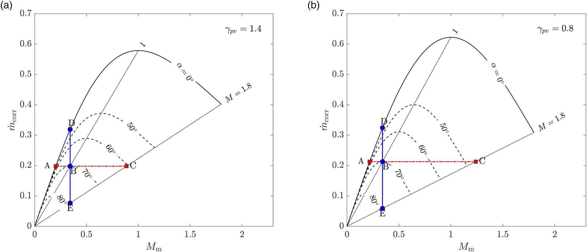
The vertical lines D-E in Figures 4a and 4b exemplify a flow expansion in which the Mach number increases from 0.5 to 1.8 at constant Mm=0.3. This process represents an expansion in a supersonic axial turbine vane designed at constant flow coefficient in which the post-expansion is negligible. During the expansion, the flow accelerates, the swirl angle increases from 0° to roughly 80°, and the corrected mass flow rate decreases because of the corresponding increase of annulus area. The reduction of m˙corr and the associated increase of annulus area is more pronounced with decreasing values of γpv, as a direct consequence of the increase in volumetric flow ratio ρt/ρ. This finding corroborates the previous results: the design of an efficient stator expanding a flow in dense-vapor thermodynamic states is arguably more challenging to accomplish.

Computational results

Methodology

The qualitative outcomes of the theoretical analysis have been verified by performing RANS simulations of a representative cascade. Figure 5 shows the computational domain of the blade vane investigated in this study. The blade corresponds to the mid-span profile of the iMM-Kis3 turbine stator designed by Giuffré and Pini (2021). Table 2 lists the main specifications of the baseline axial stator, which consists of 42 blades in total, and is designed to work at total-to-static loading coefficient of
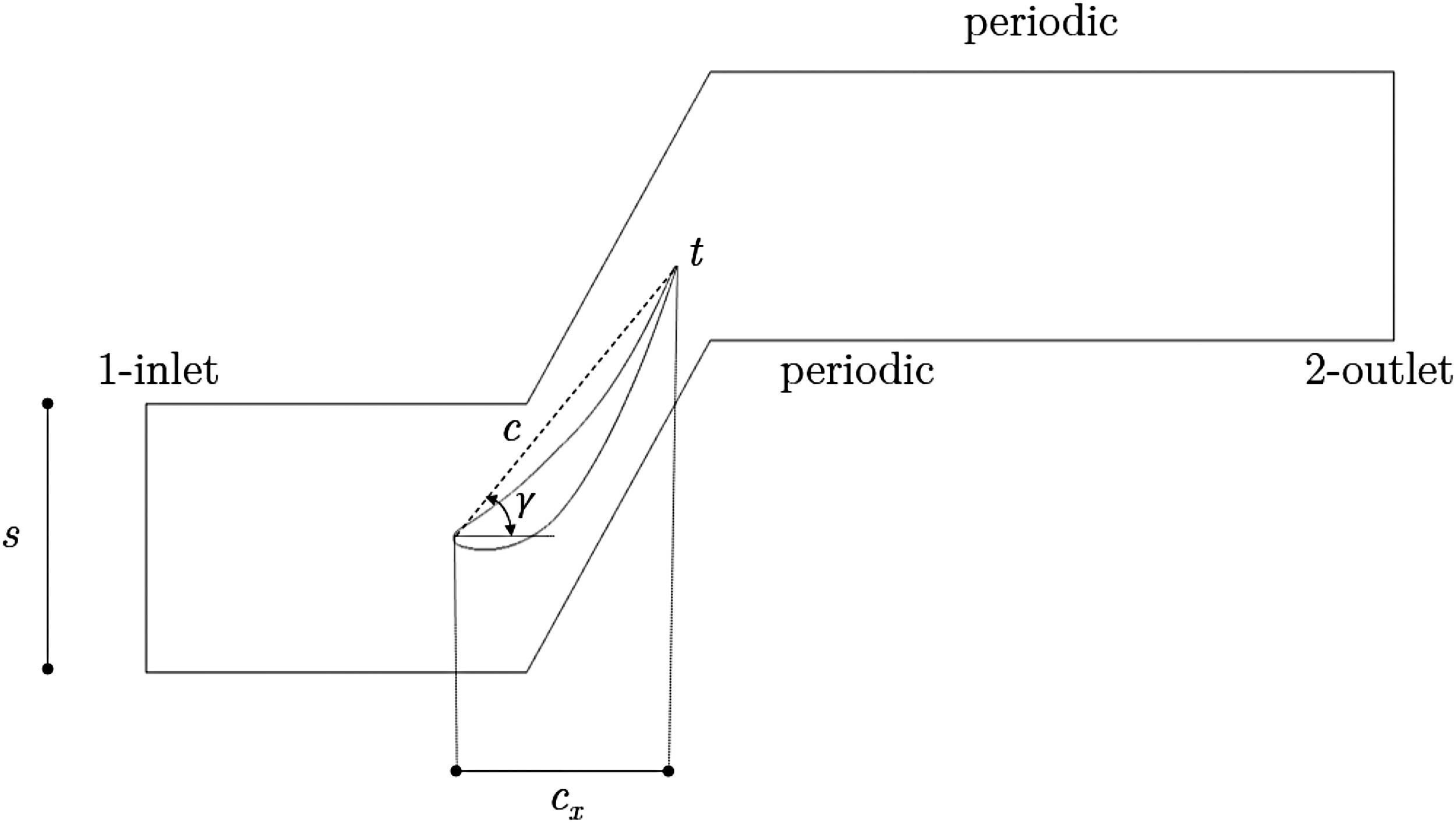
 Kis=3, flow coefficient of ϕ=0.55 and total-to-static degree of reaction of χ=0.3.

Figure 5.

Sketch of the iMM-Kis3 turbine blade and relative flow domain.

https://journal.gpps.global/f/fulltexts/151659/JGPPS-00129-2022-02.05_min.jpg
Table 2.

Geometry features of the iMM-Kis3 turbine stator blade. Here, t denotes the trailing edge thickness. See Figure 5 for the nomenclature.

c [m]cx [m]γ [o]s [m]α1 [o]α^ [o]t [mm]σx
0.02050.012650.720.0172068.80.0540.73

To avoid upstream effects and enhance mixing downstream of the blade, the inlet and the outlet of the domain have been placed 1.5cx upstream of the leading edge and 3.5cx downstream of the trailing edge, respectively. Four different working fluids are considered, namely air (ideal gas), carbon dioxide (CO2), cyclopentane and siloxane MM. Table 3 lists the cases considered in this study. For each test case, i.e., for each fluid, simulations with increasing values of βts (and thus of αts) have been carried out. The βts values have been chosen such that all regimes, from choking onset at the throat (Ma=1) to proximity of critical choking (Mx,20.9) are simulated.

Table 3.

Test cases considered in this study. Total inlet conditions are normalized with the critical pressure and temperature of each fluid. The Reynolds number Re2 is computed using the outlet flow conditions and the blade chord as reference length.

casefluidTt,in,rpt,in,rZt,inβtsαtsRe2[×106]
airair ideal gas3.560.391.02.4–4.01.9–2.71.5–1.3
iCO2carbon dioxide3.01.01.02.3–4.12.0–3.33.8–3.1
iCPcyclopentane1.00.251.02.1–3.72.1–3.72.7–2.1
iMMsiloxane MM1.030.50.842.0–3.62.2–4.03.7–2.9
niMM1.0451.30.411.6–3.22.35–5.711.8–8.1

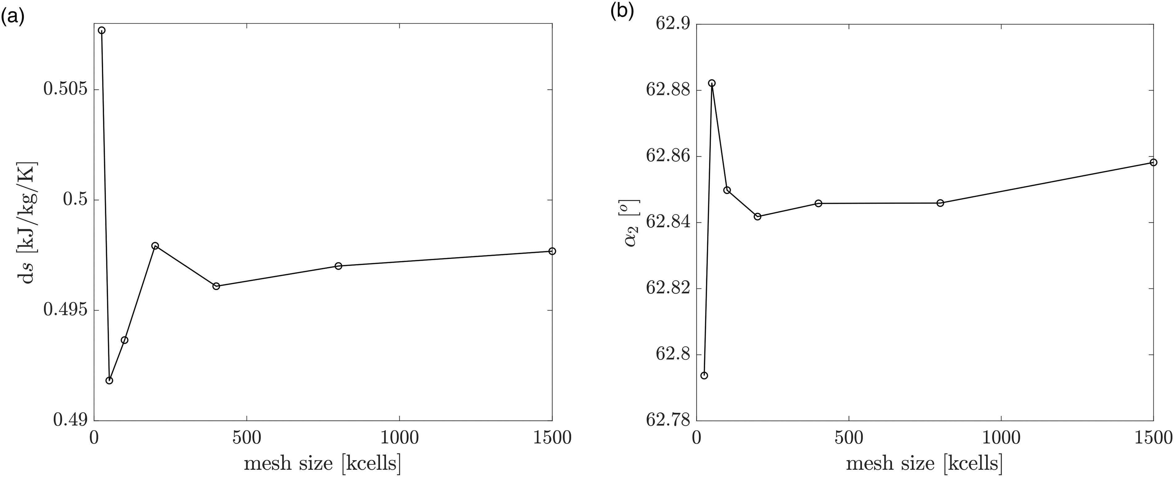
The domain was meshed with quadrilateral elements using the commercial grid generator of a well-known CFD software package (ANSYS, 2019). To ensure proper mesh resolution, both local refinement in proximity of the blade walls and average cell size are kept constant for all the investigated cases. The average cell size in the flow domain is set to 3.75105m. Cell clustering is introduced near the blade walls to guarantee y+<1. To ensure compatibility with the three-dimensional solver, the mesh has been extruded of 5106m along the spanwise direction. Figures 6a and 6b show the results of the grid independence study conducted for the case niMM at βts=1.75. For this study, results obtained with a mesh of 200k cells are deemed grid independent. The SST kω model is employed to compute the turbulent stresses as commonly done in these cases (Anand et al., 2018). To ensure that all the flow processes occur in the dilute gas state (Z1), except for the niMM case), total pressure and temperature are prescribed at the domain inlet according to the values reported in Table 3. The desired total-to-static pressure ratio is obtained by fixing the value of the static pressure at the outlet. No-slip conditions are established at the blade walls. Translational periodic interfaces are set at the upper and lower bounds of the domain, while symmetry boundary conditions are assumed on the two remaining interfaces. A turbulent intensity value of 5% and a turbulent viscosity ratio μT/μ=10 were used throughout this study. The turbulent Prandtl number is set to Prt=0.9, in accordance with Otero et al. (2018). The advective fluxes are discretized with total variation diminishing schemes. Turbulent fluxes are discretized with a first order upwind scheme. A central difference scheme is used to discretize the viscous fluxes. The fluid properties are calculated with a look-up table approach, resorting to a well-known library for the estimation of thermophysical properties (Lemmon et al., 2018).

Figure 6.

Mesh sensitivity analysis. (a) Entropy generation across the vane (ds=s2s1) vs mesh size. (b) Outlet flow angle vs mesh size.

https://journal.gpps.global/f/fulltexts/151659/JGPPS-00129-2022-02.06_min.jpg

The values of the deviation obtained from CFD simulations are compared against those obtained from a reduced-order model (ROM). Following the analysis proposed by Denton (1993), the ROM is based on a control volume approach to estimate the entropy generation due to mixing and the flow deviation downstream of the passage throat. Figure 7 shows the control volume used for the calculations. The volume is enclosed between the location of the throat (a) and the outlet section over which the flow is assumed to be fully mixed (mo). The flow at the throat is chocked, i.e., Ma=1. The flow properties at the throat are calculated knowing the values of the inlet total conditions, according to Table 3, and the entropy sa evaluated at the throat. sa is computed as the sum of the entropy generated within the blade boundary layers Δsbbl and the entropy sin at the passage inlet. The Δsbbl value is calculated using the reduced-order model described by Giuffré and Pini (2021). With reference to the nomenclature in Figure 7, the mass conservation, axial momentum balance, tangential momentum balance and energy conservation equations for the considered control volume read, respectively,

(8)
ρaVa(aδ)=ρmoVmocosαmos=m˙,
(9)
paa+pbt+psslsinψ+m˙VaρaVa2θs=m˙Vmocosδ+pmocosαas,
(10)
psslcosψ=pmosinαas+m˙Vmocosδ,
and
(11)
m˙(ha+Va22)ρaVa32θ=m˙(hmo+Vmo22).
where δ=αmoαa, αa being the gauge angle, i.e. αaarccos(a/s), and αmo the flow angle at the outlet. pss denotes the pressure acting over the rear length of the blade suction side, while ψ identifies the angle between the camber line at the trailing edge and the segment l connecting the trailing edge to the intersection between the throat and the suction side. For simplicity, we assumed ψ=0 for all the cases investigated in this work. At the trailing edge, the displacement thickness δ, the momentum thickness θ, and the kinetic energy thickness θ are taken into account. Average values of these quantities have been set according to the results of the numerical simulations conducted in this work, i.e., δ/θ=1.6, θ/t=0.075, and θ/t=0.085. The base pressure has been calculated according to correlations by Sieverding and Manna (2020). The system of equations is closed by a multiparameter equation of state (EoS) model (Lemmon et al., 2018). Given the outlet pressure pmo from the fixed βts values listed in Table 3, the solution of the system of equations provides the value of both the deviation δ and the mixing losses, which are computed as
(12)
ζmix=TmoΔsmixht,mohmo,
where Δsmix=smosa denotes the entropy generation between the mixed out section and the throat.

Figure 7.

Control volume used for the estimation of flow deviation and mixing losses.

https://journal.gpps.global/f/fulltexts/151659/JGPPS-00129-2022-02.07_min.jpg

Shock losses within the mixing region are estimated using the Rankine-Hugoniot relations for a dense vapor fluid (Vimercati et al., 2018). The post-shock entropy sshock is calculated knowing the values of both Mach number and pressure upstream of the shock and that of the shock angle. Relations for both the shock angle and the pre-shock state as a function of the fluid and βts have been developed by correlating the results of the RANS simulations performed in this study. The shock loss coefficient is then calculated as

(13)
ζshock=TmoΔsshockht,mohmo,
where Δsshock=sshocksa denotes the entropy generation between the post-shock state and and the throat.

Flow deviation

Figure 8a shows the flow deviation downstream of the trailing edge as a function of the total-to-static volumetric flow ratio. For the dilute gas cases, the deviation increases with αts, with moderate quantitative differences among the various fluids (14% at αts=3.25). The trends predicted by the mixing model are in good agreement with those obtained with CFD, with the ROM slightly underestimating the value of δ. The niMM case, instead, is characterized by values of deviation at fixed αts that are lower by approximately 42% at αts=4, as compared to those calculated for the iMM case. In summary, for a fixed value of the volumetric flow ratio, the flow deviation decreases with both the fluid molecular complexity and the degree of thermodynamic non-ideality, as measured by the average value of γpv over the expansion process. The opposite trend occurs if the deviation is plotted as a function of the outlet Mach number M2 (Figure 8b), i.e., δ increases when the average value of γpv decreases, for the same value of M2.

Figure 8.

Flow deviation at the blade trailing edge vs volumetric flow ratio (a) and outlet Mach number (b) for the cases reported in Table 3. Continuous and dashed lines denote results of CFD and of the reduced-order model, respectively. Values of the measured axial Mach number are also reported.

https://journal.gpps.global/f/fulltexts/151659/JGPPS-00129-2022-02.08_min.jpg

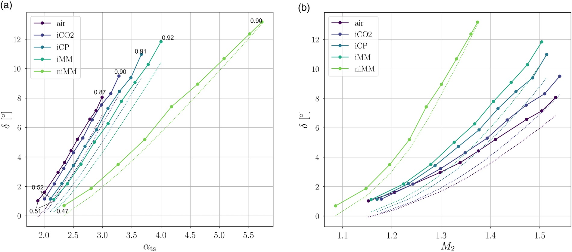
Figure 8b also shows that the expansion needed to obtain an axial Mach number of 0.9 and, consequently, the critical choking of the cascade, decreases with the molecular complexity of the fluid and the thermodynamic non-ideality. When the thermodynamic state of siloxane MM approaches that of the critical point, the Max=0.9 condition is reached at M1.38. Conversely, for the case iMM, such condition is reached at M1.5. Figure 9a displays the Mach number contours in both the vane passage and the wake for the three cases: air, iMM and niMM at constant outlet Mach number. For the same cases, the blade loading is also depicted in Figure 9b. The streamlines highlight that the flow deviation increases with the complexity of the working fluid and while approaching the dense vapor state.

Figure 9.

(a) Detail of the flow at the blade trailing edge at M2=1.36. Streamlines are traced in proximity of the blade surface to highlight the flow deviation. (a) air, βts=3.2 (b) iMM, βts=2.8, (c) niMM, βts=3. (b) Isentropic Mach number distribution over the blade for three different cases at fixed M2=1.36.

https://journal.gpps.global/f/fulltexts/151659/JGPPS-00129-2022-02.09_min.jpg

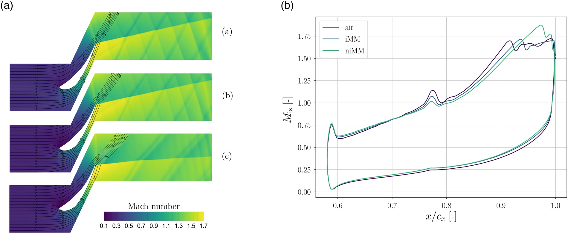
Given the higher average value of γpv in the iMM expansion, the margin with respect to critical choking is larger if compared to the niMM case, in agreement with the results presented in Sec. 2. Conversely, when γpvγ (the niMM case, in this study), the critical choking onset occurs at lower Mach numbers, limiting thus the operability of the cascade. The reason why the flow deviation increases with Mach number, fluid molecular complexity and thermodynamic non-ideality can be inferred from an analogy with one-dimensional nozzle flows. For an arbitrary fluid, the area variation needed to obtain a desired Mach variation reads (Thompson, 1971)

(14)
dAA=1M21+(Γ1)M2dMM

where Γ is the fundamental derivative of gas dynamics. Given a supersonic expansion at fixed inlet Mach number, the nozzle area increase dA required to obtain a fixed outlet Mach number is inversely proportional to Γ. Similarly to nozzle flows, for fluids operating in states where the Γ value is low, the expansion through a converging turbine cascade requires a larger post-expansion cross-section. The flow rotation due to the expansion fan at the trailing edge determines the entity of the flow deviation during post-expansion in the unguided region. Both fluid molecular complexity and thermodynamic state affect the entity of the rotation, which is described by the Prandtl-Meyer function ν(M). For a dense vapor fluid, an approximated relation for ν(M) can be retrieved by solving the conservation equations and using the thermodynamic relations by Baltadjiev et al. (2015). This yields

(15)
ν(M)=(M21)(1+γpv12M2)1dMM.

Equation 15 holds under the assumption of constant γpv between static and stagnation quantities; this condition is usually satisfied if the state of the fluid is far from the vapor-liquid critical state, where large gradients of γpv do not occur. If γpv is assumed constant and >1, Equation 15 can be integrated to obtain

(16)
ν(M)=γpv+1γpv1arctanγpv1γpv+1(M21)arctanM21.

which differs from the canonical ideal gas version for the presence of the isentropic exponent γpv in place of γ. The value of the Prandtl-Meyer function increases with decreasing γpv, leading thus to increased flow turning at a fixed supersonic outlet Mach number. Experimental and numerical results by Durá Galiana et al. (2016) confirm this trend.

Large flow deviations have relevant implications for turbine design and operation. Larger deviations imply higher axial Mach numbers, thus limiting the maximum allowable stage volumetric flow ratio. Moreover, off design operation becomes more challenging as critical choking occurs at lower Mach number. Furthermore, an incorrect prediction of the flow deviation can lead to a sizeable offset in the power output of the turbine at design point.
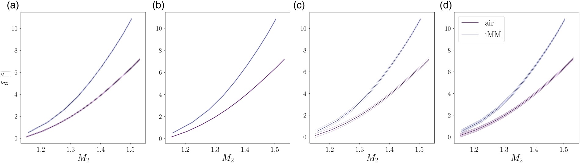
For completeness, Figures 10a10c show the sensitivity of the deviation to variations in displacement thickness, momentum thickness, kinetic energy thickness and base pressure coefficient. Results are reported for air and siloxane MM (case iMM). In each graph, each parameter is varied by ±50% with respect to the baseline value, while the other two parameters are kept constant. For a fixed trailing edge thickness to pitch ratio, the influence of δ/θ, θ/t and θ/t on the flow deviation is negligible. For the air case, the maximum calculated variation is 3% for δ/θ, 1.5% for θ/t, and 4% for θ/t. Larger discrepancies are observed in case of variations of the base pressure coefficient (Figure 10c), with the largest offset being 28% for air at M2=1.25.

Figure 10.

Sensitivity of the flow deviation to parameters of the ROM for the air and iMM cases. Sensitivity to (a) δ/θ, (b) θ/t, (c) θ/t and (d) base pressure coefficient pb. The continuous red line is the deviation value obtained using the baseline value for each parameters. The shaded areas highlight the influence of each parameter if varied by 50% with respect to its baseline value.

https://journal.gpps.global/f/fulltexts/151659/JGPPS-00129-2022-02.10_min.jpg

Loss breakdown

The analysis has been complemented by comparing the loss trends computed with the models derived from first principles and the ones extracted from CFD simulations. The two investigated loss mechanisms are dissipation due to viscous stresses in the boundary layer, and viscous mixing occurring downstream of the trailing edge.

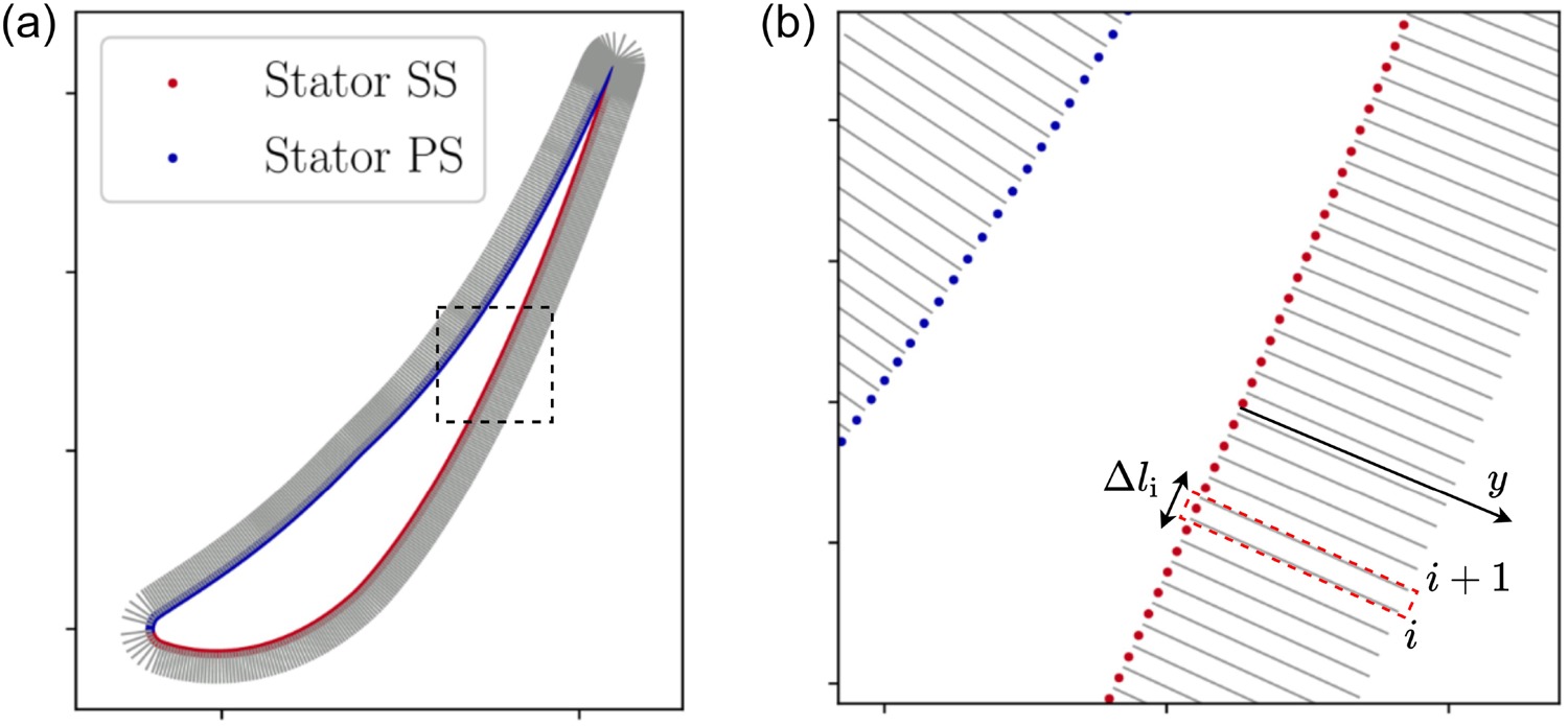
The boundary layer loss obtained from CFD simulations is computed according to the methodology described by Duan et al. (2018). With reference to Figure 11, first, the blade surface is partitioned into segments (Δli) and, for each couple of adjacent grid points (i and i+1), the normal to the surface is calculated. Then, for each point along the normal direction, the values of the flow quantities ρ,V,T,s are extracted by interpolating the simulation results evaluated at the adjacent grid points. This process is iterated up to the edge of the boundary layer, which is here deemed as the location where s/y0. The entropy production rate per unit area within each control volume defined by two adjacent normals can then be computed using the second law of thermodynamics as

Figure 11.

Computation of blade boundary layer loss from CFD data. (a) Evaluation of normals to the blade surface. (b) Calculation of entropy generation in each control volume through numerical quadrature.

https://journal.gpps.global/f/fulltexts/151659/JGPPS-00129-2022-02.11_min.jpg
(17)
S˙=ddx0δblρV(sse)dy.

The local value of the dissipation coefficient can be calculated by normalizing the entropy production rate as

(18)
Cd=TeS˙ρeVe3,

and the overall specific entropy production due to boundary layer friction can be approximated as

(19)
Δsbbl=1m˙bladeCdρeVe3Tedl1m˙iCd,iρe,iVe,i3Te,iΔli.

The boundary layer dissipation can finally be computed as

(20)
ζbbl=T2Δsbblht,2h2.

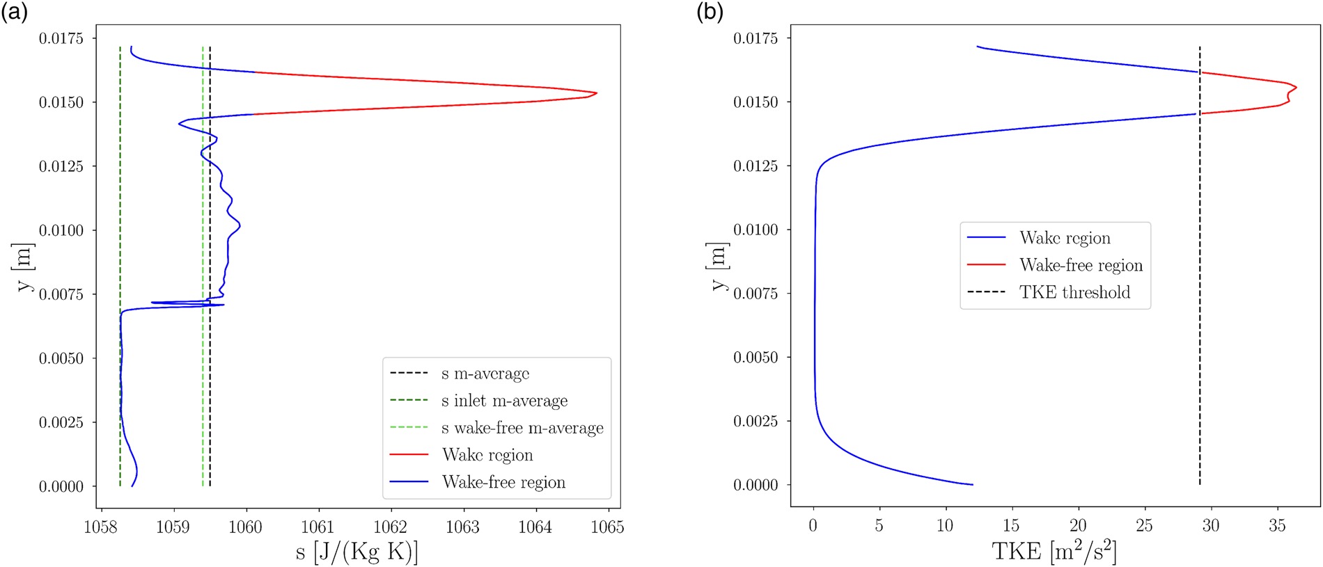
Once the dissipation due to blade boundary layer friction is known, the remaining two-dimensional losses are divided in two components, see Mee et al. (1992): wake-free losses and wake-induced losses. Wake-induced losses are those related to the trailing edge base region and the mixing of boundary layers downstream of the blade row. The wake region is identified by inspecting the pitch-wise trend of the turbulent kinetic energy k extracted from the CFD results at x=xte+0.5cx, as displayed in Figure 12b. The mass flow averaged entropy s¯w computed using entropy values at pitch-wise locations where κ>0.7κmax is used to calculate the wake-induced loss coefficient, (see Figure 12a), defined as

Figure 12.

(a) Entropy and (b) turbulence kinetic energy profile evaluated at x=xte+0.5cx for test case iMM, βts=2.4. The entropy profile is used to compute shocks-induced loss from CFD data.

https://journal.gpps.global/f/fulltexts/151659/JGPPS-00129-2022-02.12_min.jpg
(21)
ζw=T2Δswht,2h2,

where Δsw=s¯ws1Δsbbl. On the other hand, the entropy increase corresponding to κ<0.7κmax is mass flow averaged to obtain the wake-free loss coefficient, defined as

(22)
ζwf=T2Δswfht,2h2,

where Δswf=s¯wfs1Δsbbl and s¯wf is the mass flow averaged wake-free entropy.

The stacked plots in Figure 13 show the results of the loss breakdown analysis for the iMM (Figures 13a and 13b) and the niMM (Figures 13c and 13d) test cases. In particular, Figures 13a and 13c display the contribution of boundary layer, wake-free and wake losses extracted from the CFD simulations, together with the overall loss computed with the ROM, for comparison purposes. Conversely, Figures 13b and 13d display the contribution of boundary layer, shock and mixing losses estimated with the ROM described in Sec.3.1, together with the total passage loss calculated by the RANS simulations. The trend of the total passage loss estimated with CFD is in agreement with that calculated with the ROM. However, the ROM underestimates the total loss, and the deviation scales with the outlet Mach number. This offset can be attributed to the shock loss model, which takes into account only the contribution of the main shock downstream of the trailing edge and does not account for the entropy generation due to secondary and reflected shocks, see Figure 9a.

Figure 13.

Loss breakdown for the (a-b) iMM and (c-d) niMM cases. Loss estimations from (a-c) CFD results and (b-d) ROMs of Sec. 3.1 are reported for both cases. The total passage loss estimated with (a-c)) ROMs and (b-d) CFD results are also reported in dashed lines.

https://journal.gpps.global/f/fulltexts/151659/JGPPS-00129-2022-02.13_min.jpg

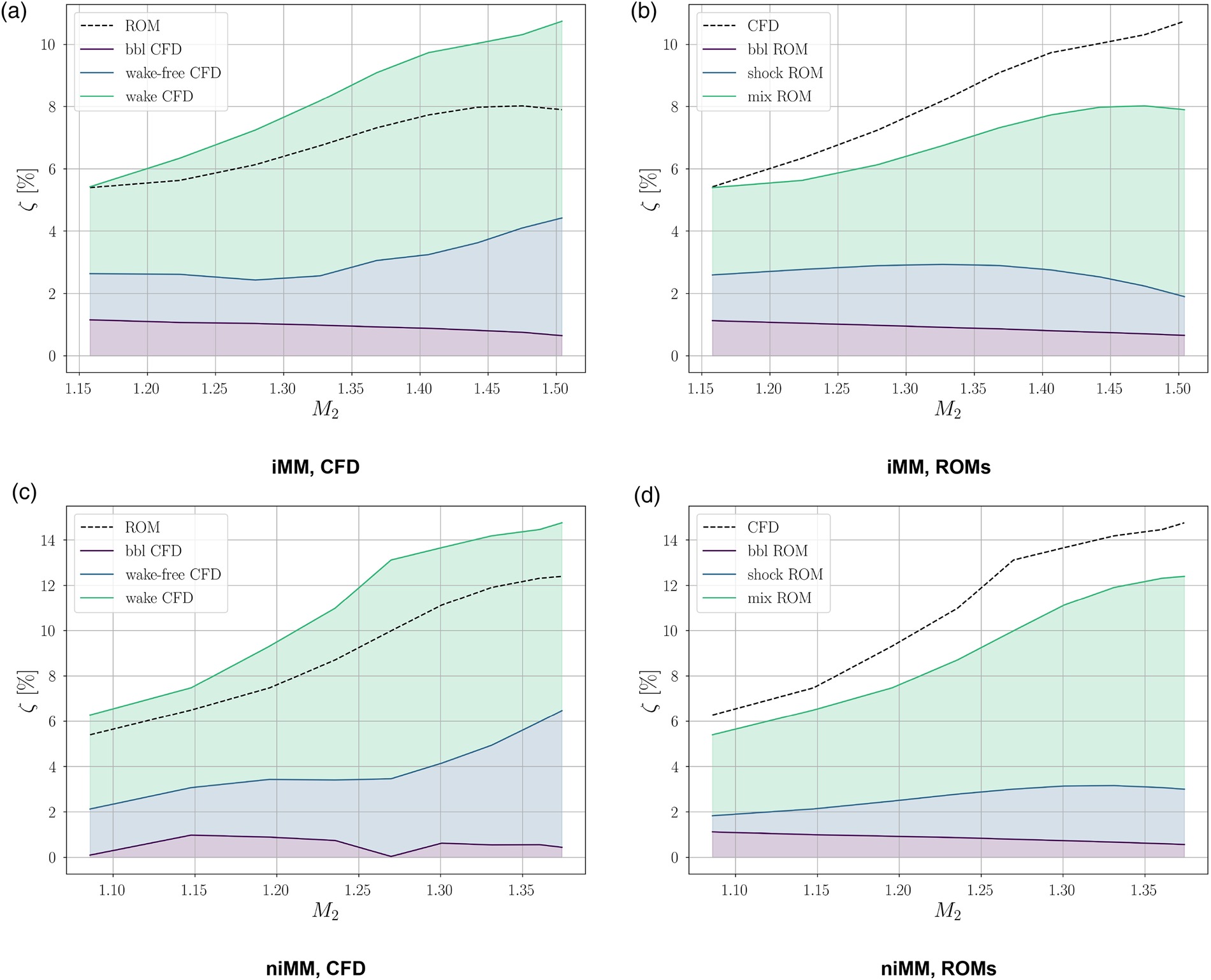
Figure 14a displays the variation of the values of specific entropy generation due to viscous effects in boundary layers as a function of the outlet Mach number for the cases of Table 3. The figure presents a comparison between results obtained with the reduced-order model developed by Giuffré and Pini (2021) and those calculated by means of CFD simulations. Both models predict that boundary layer losses decrease with the outlet Mach number. Except for the non-ideal case niMM, in all other cases the predicted value of dissipation at a fixed M2 is rather similar. At M2=1.4, the maximum variation between the various cases is <2%. Lower boundary layer losses are predicted in case the flow is non-ideal (niMM). The motivation is twofold. First, the fluid undergoing an expansion from a dense vapor state is affected by a larger density gradient if compared to a similar expansion in the ideal gas state. As a consequence, the specific entropy production rate, which depends also on the density gradient along the blade surface, is larger in the niMM case, see Equation 17. In turn, the difference between the two values is due solely to thermodynamics, given that the blade loading is almost constant at fixed outlet Mach number for all the considered cases, see Figure 9b. Second, at fixed blade loading, the value of the Reynolds number of the cascade is lower for expansions of fluids made of simple molecules in the dilute gas state and larger for expansions of dense organic vapors, see Table 3. As a consequence, lower values of dissipation coefficient and, thus, of fluid-dynamic loss, characterize dense vapor expansions.

Figure 14.

Blade boundary layer loss (a) and trailing edge loss vs (b) outlet Mach number M2 for the cases reported in Table 3. Continuous and dashed lines denote results of CFD and ROM, respectively.

https://journal.gpps.global/f/fulltexts/151659/JGPPS-00129-2022-02.14_min.jpg

Figure 14b shows the trend of the loss coefficient ζnobbl due to dissipation occurring in the free-stream and in the wake region as a function of the outlet Mach number, for the cases of Table 3. In the CFD loss breakdown framework, the dissipation accounts for wake and wake-free losses, while in the ROM it accounts for mixing and shock losses downstream of the throat. The dissipation increases with the outlet Mach number for all the considered cases. Moreover, flows of fluids made of complex molecules are affected by larger mixing losses. Results from CFD simulations and from the ROM are qualitatively in agreement. However, at fixed M2, the ROM underestimates the losses compared to CFD simulation results. At M21.4, the loss coefficient estimated by the two models differs by 2%. This discrepancy can be arguably attributed to the fact that the shock loss model does not account for the entropy generation due to shock wave reflection and secondary effects, i.e., boundary layer-shock interactions. Moreover, both methods predict a larger loss coefficient at fixed outlet Mach number for the niMM case compared to the dilute gas cases. At M2=1.36, the mixing loss calculated for the niMM case is 6% larger than the corresponding dilute gas case, i.e., iMM. Free-stream and wake losses are considerably larger than boundary layer losses, which are on the order of 1%. ζnobbl is also plotted as a function of the volumetric flow ratio αts in Figure 15a. Remarkably, ζnobbl becomes only a function of αts, regardless of the working fluid and the thermodynamic state. This is in line with the findings by Giuffré and Pini (2021).

Figure 15.

(a) Mixing loss vs volumetric flow ratio αts for the cases reported in Table 3. Continuous and dashed lines denote results of CFD and ROM, respectively. The dashed black line depicts a quadratic fit of the data; the fitted equation is reported in the Appendix. (b) Mixing loss vs throat-to-outlet density ratio according to the simplified model of Equation 26.

https://journal.gpps.global/f/fulltexts/151659/JGPPS-00129-2022-02.15_min.jpg

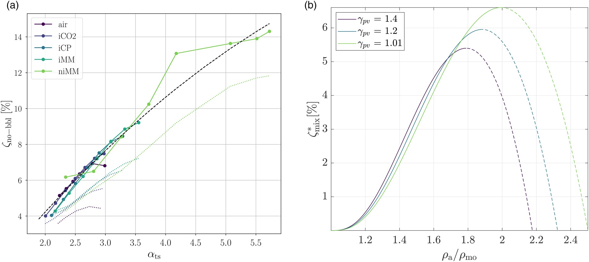
The effect of the fluid molecular complexity and of the thermodynamic state on the mixing loss can be analytically evaluated by using a simplified version of the mixing model introduced in Sec. 3.1, see Osnaghi (2002). By neglecting the contributions of both the base pressure and the boundary layer quantities δ and θ, and by assuming Ma=1 at the throat and by also assuming that a general equation of state model in the form pv=ZRT holds, one can predict the flow deviation according to

(23)
tanδ=((γpv)/(γpv1))(pmo/pa)tanαa1+γpv(pmo/pa)+((γpv+1)/(γpv1))(1(pmo/pa))2+(((γpv)/(γpv1))(pmo/pa)tanαa)21+γpv(pmo/pa),
(24)
VmoVa=1cosδ[1+1γpv(1pmopa)],
and
(25)
ρaρmo=papmo[1+γpv12(1Vmo2Va2)],
where pmo/pa is the independent variable. Also here, relations between stagnation and static variables p, T and Z have been estimated with the equations proposed by Baltadjiev et al. (2015). The approximated mixing loss can then be calculated as
(26)
ζmix=(((γpv+1)/2))((γpv)/(γpv+1))(pmo/pa)(1+((γpv1)/2)Mmo2)((γpv)/(γpv+1))(((γpv+1)/2))((γpv)/(γpv+1))1.
Figure 15b shows the variation of the mixing loss with the throat-to-outlet density ratio, according to Equations 25 and 26. To account for both fluid molecular complexity and thermodynamic non-ideality, results are reported for three different values of the γpv exponent. The maxima of the curves identify the Mmo,x=1 condition, i.e., critical choking. The plots show that, for ρa/ρmo<1.7, the mixing is unaffected by the value of γpv. This result is in qualitative agreement with those reported in Figure 15a. However, the maximum of the curves increases with decreasing values of γpv. Values of γpv1 characterize complex organic fluids such as siloxane MM, and these values decrease if the thermodynamic state of the fluid approaches that of the critical point. This is also in line with the trends that can be observed in Figures 14b.

Conclusions

This paper documents an investigation on the flow deviation in transonic turbine cascades operating with non-ideal compressible flows. The definition of corrected mass flow per unit area has been extended to the case of swirling flows in the non-ideal compressible flow regime. The onset of critical choking, i.e., sonic meridional flow at the cascade outlet, and its relationship with flow deviation have been discussed. The influence of the working fluid on the corrected mass flow per unit area, the critical choking occurrence in transonic cascades and the flow deviation at blade trailing edge have been both theoretically and numerically investigated. Reduced-order models for the estimation of the flow deviation and the preliminary assessment of the two-dimensional losses have been derived and validated against the results of CFD simulations. The influence of the working fluid and of the thermodynamic state throughout the expansion has been assessed and quantified with the value of the generalized isentropic exponent γpv. Based on the outcomes of the work, the following conclusions can be drawn.

  1. It is theoretically predicted that lower γpv values over the expansion entail a lower expansion ratio for the flow to reach critical choking conditions. Furthermore, the flow deviation substantially increases if γpv<γ.

  2. Results from CFD simulations of the flow through a representative ORC turbine cascade corroborate the findings of the theoretical analysis. In particular, it is found that the reason of the increased flow deviation can be explained by means of the Prandtl-Meyer function.

  3. The proposed reduced-order model provides accurate trends of flow deviation and mixing loss if compared to the values obtained from CFD simulations. Therefore, the reduced-order model can be used to predict the flow deviation during the preliminary design phase of unconventional axial turbines.

  4. The value of expansion ratio that leads to critical choking decreases with increasing thermodynamic non-ideality and molecular complexity of the fluid. This has consequences on the maximum expansion ratio for which the stage can be designed. For example, for a turbine cascade operating with siloxane MM in thermodynamic conditions similar to those of the niMM test case, the total-to-static expansion ratio cannot exceed 3.

  5. The total loss increases with flow compressibility, fluid molecular complexity and decreasing values of the generalized isentropic exponent γpv. The largest share of total loss is due to mixing of wakes in the trailing edge region and the presence of shock waves.

  6. It is found that the volumetric flow ratio is the most suited scaling parameter for cascade loss and flow deviation, regardless of the working fluid and the thermodynamic conditions.

Future work will address the study of the flow deviation in supersonic cascades for axial and radial turbines operating with non-ideal compressible flows. Experimental validation will also be paramount to provide confidence on the findings of this work.