Introduction

Aircraft engines are exposed to a variety of external influences during operation causing gradual engine deterioration and damages over operation time (Kellersmann et al., 2018). Main influences concerning the engines high pressure compressors are deposition and erosion due to airborne particles (Richardson et al., 1979). To predict realistic erosion as well as deposition patterns, accurate modelling of the particle rebound after impacting a surface is indispensable.

Particle rebounds are statistical in nature due to varying particle sizes, particle shapes, target surface topography, particle rotation and particle break-up during contact. Existing modelling approaches based on empirical correlations fail to predict the spread in the coefficients of restitution (CoR) at different operating conditions than the original experimental setup by up to 100% (Bons et al., 2015). Furthermore, present modelling approaches based on physical considerations have focused on modelling particle impacts mean rebound coefficients only. Standard deviations of the coefficients of restitution vary with the considered particle and target surface combination. Hence excessive experimental testing of different particle-surface combinations is needed to simulate the statistical spread numerically. The scope of the presented work is to access the statistical spread of particle rebound data through analytical considerations. For simplification only statistical spread of particle rebound due to target roughness will be discussed here as a first step towards a general physical based spread model. The presented approach is based on work of Sommerfeld and Huber (Sommerfeld and Huber, 1999). It derives local impact angles α1′ due to surface roughness for individual particles, which may deviate by Δα from the global impact angle α1 as shown in Figure 1. It can be combined with an existing rebound model like the one presented by (Bons et al., 2017) (Figure 2).

Figure 1.

Determination of velocities and angles before and after impact.

Figure 2.

Diagram of model implementation in a closed modelling loop.

Further input variables for the Bons-Model are used according to (Whitaker and Bons, 2018) for ARD particles in a 1–100 μm size distribution.

Theoretical background

Usually coefficients of restitution are used to describe the energy loss during collision. They are defined as the magnitude of a parameter after rebound divided by its corresponding magnitude at impact (Figure 1):

To estimate these coefficients in turbomachine applications, rebound and deposition models are used. They are based either on a critical velocity approach derived by Brach and Dunn (Brach and Dunn, 1992) or a critical viscosity approach based on work of Tafti and Screedharen (Sreedharan and Tafti, 2010). Critical viscosity models concern particle softening mechanisms at high temperature applications in the turbine section and are not reviewed in this study aiming to evaluate particle impact in the engines compressors section. Deposition models based on critical velocity determine whether a particle sticks to the surface by comparing the actual impact velocity with a capture velocity for the impact event. Below this capture velocity the particle will deposit. If a particle does not deposit an estimate of the rebound velocity is applied.

These models are based on contact mechanics with elastic deformation in a Hertzian contact of a spherical particle with a flat surface in normal direction combined with adhesion during impact (Brach and Dunn, 1992). This approach has been extended to account for oblique impacts, elastic-plastic deformation and further external forces (Kim and Dunn, 2007; Singh and Tafti, 2015; Barker et al., 2017). Still it is valid for spherical particles only and rely heavily on empirical correlation (Bons et al., 2017).

Therefore Bons et al. (Bons et al., 2017) derived a quasi-physical but yet equally empirical and approximate modelling approach based on representing arbitrary particle shapes as a circular cylinder. It allows to model particle deformation as a 1D spring rather than a complex 3D deformation of a sphere. The model comprises elastic and plastic deformation, adhesion, and shear removal. It has been further improved by Whitaker (Whitaker and Bons, 2018) to account for stochastic spread of rebound data with an empirical curve fitting approach based on experimental data. Since this approach still relies on excessive experimental testing of different material and particle combinations a physical based access to the statistical spread due to surface roughness is desired in this work. Based on roughness profiles which have been found at deteriorated surfaces a sensitivity study has been conducted. The results of the sensitivity study will be discussed after introducing the developed modelling approach to statistical spread.

Surface roughness modelling

Characteristic roughness profiles for performance deterioration in turbomachinery components can be found in (Bogard et al., 1998; Bons et al., 2001; Syverud et al., 2005; Gilge et al., 2019). Based on their published data a Design of Experiments (DoE) has been carried out in this work:

The roughness root mean squared R_q and correlation length λ_c were used to characterize roughness height and elongation of the examined surface (Figure 3). The roughness profiles were processed with a morphological filter routine based on the closing principle (Serra and Vincent, 1992). The filtered profile defines how deep a particle of size dP impacting normal to the surface (90°) can penetrate the roughness structure (Figure 3).

Figure 3.

Roughness topography and morphological filter.

The roughness profiles have been generated artificially using the methods outlined by Garcia and Stoll (Garcia and Stoll, 1984). This procedure utilises roughness profiles with different R_q and λ_c that fulfil the Gaussian statistics. Corresponding slope angles are obtained by applying the morphological filter as described above. In this way the filtered profile leads to the local impact angle α1′, where the particle hits the surface. By applying a kernel density estimation on the sampled data a distribution function of possible impact angles has been gained. These probability distributions of the local impact angles can be approximated with a Normal Gaussian Distribution (Sommerfeld and Huber, 1999) with the expected value µ and the variance σ². Such an approximation provides a significant saving in required storage space in the modelling process.

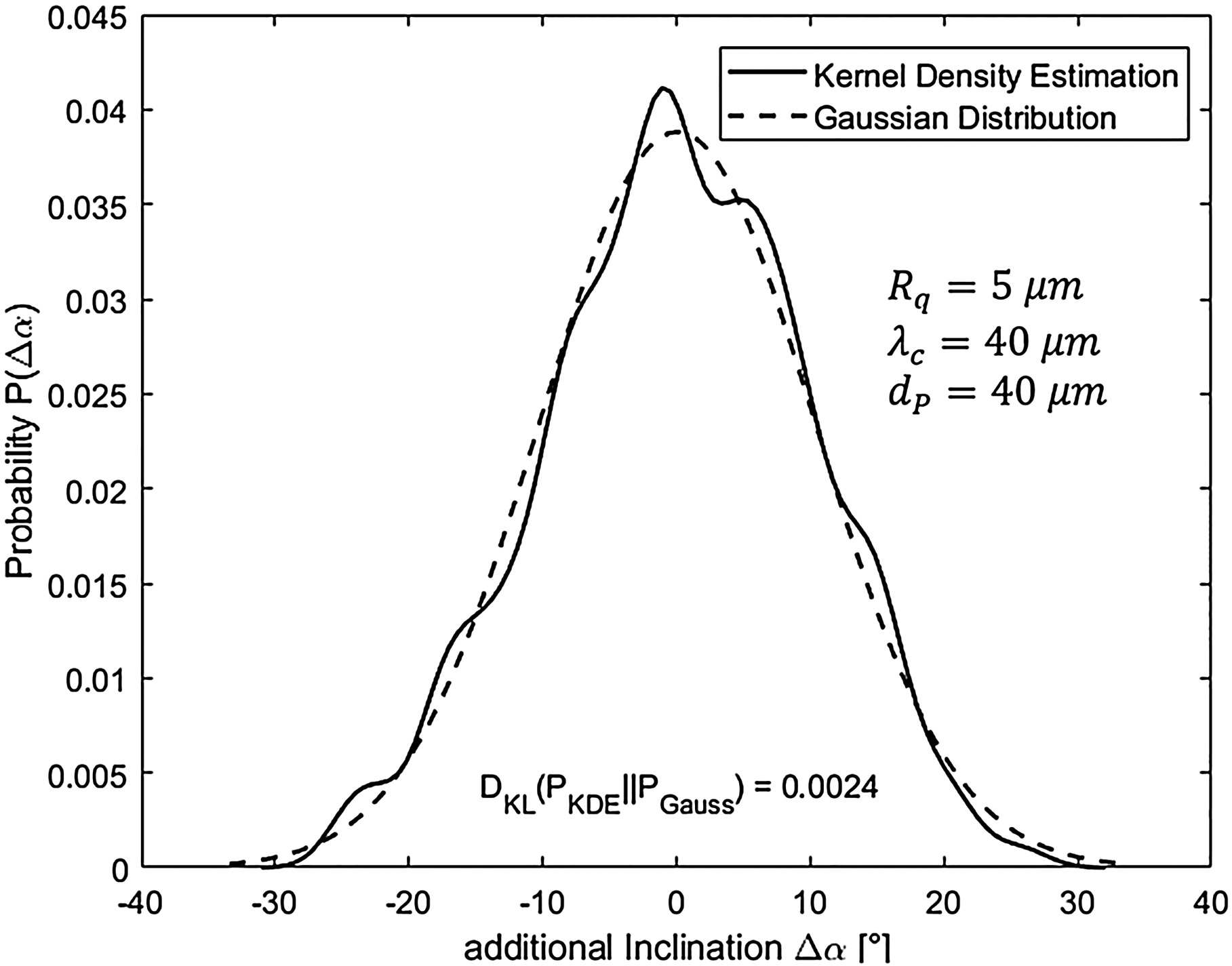
The Kullback-Leibler divergence is used to evaluate the quality of the approximation (Kullback, 1978). For values DKL close to zero, sufficient accuracy has been archived.

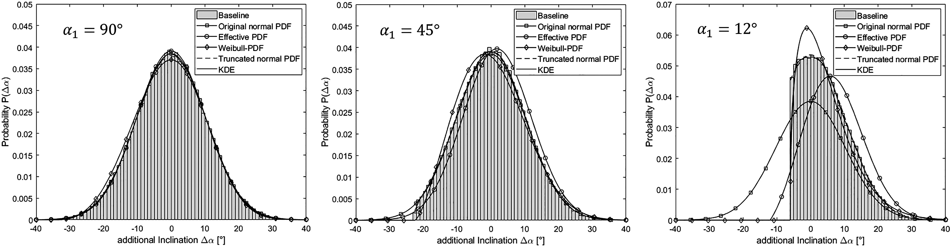
Figure 4 shows an example for the kernel density estimation and its corresponding normal Gaussian approximation. The Kullback-Leibler divergence for all generated profiles are close to zero with a median value of DKLmedian=0.0251. Hence sufficient accuracy by the approximation with a Normal Gaussian distribution has been archived.

Figure 4.

Quality of approximation.

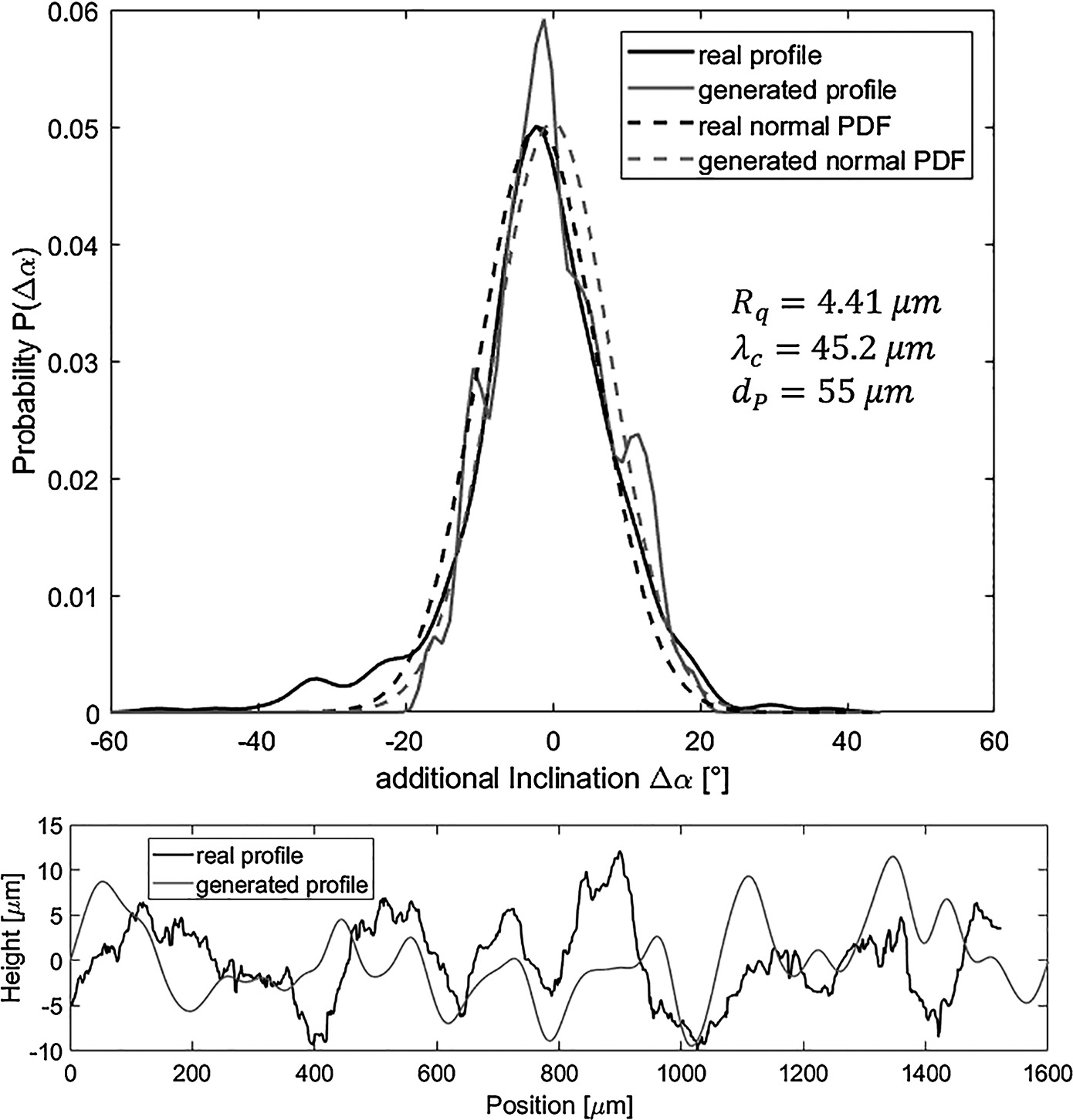
In order to validate the whole roughness generation process a surface roughness of a deteriorated compressor blade has been scanned with an optical profilometer (Talysurf CCI – Taylor Hobson) (Casari et al., 2018) and compared with an artificially created profile of the same roughness characteristics R_q and λ_c (Figure 5). With a value of DKL(Preal||Pgenerated)=0.058, the generated profile reproduces the slope angle distribution of the original profile with sufficient accuracy.

Figure 5.

Roughness estimate of deteriorated compressor blade.

Modelling the local impact angle

After discussing a particle impacting normal to the surface, the variation of the global angle α1 and its effect on the inclination angle Δα is addressed. For small impact angles α1 particles may not hit the lee side of roughness structures if the absolute value of the negative slope angle becomes larger than the impact angle. This leads to a higher probability to hit the luff side of a rough structure and as a result to a shift of the probability distribution of the additional inclination angle Δα towards positive values. To evaluate this phenomena (Sommerfeld and Huber, 1999) proposed a simulation methodology (baseline) which is subject to the following three routines:

The last step leads to the restriction that no negative inclination Δα with absolute values larger than α1/2 is valid.

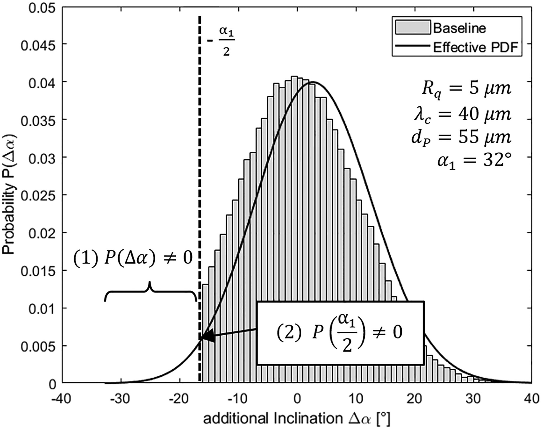
In order to avoid this time consuming iteration loop in numerical simulations (Sommerfeld and Huber, 1999) proposed that this so called “shadow effect” can be described by an effective probability distribution function

The term ξ(α1,σ) achieves the normalization of the manipulated Probability Distribution Function (PDF). However the straight forward use of this effective PDF Peff(α1,σ,Δα) might lead to unphysical results. As can be seen in Figure 6 two main issues occur: (1) The effective PDF defines a non-zero probability for local roughness angles smaller than the limit α1/2. This leads to a particle rebound towards the wall. (2) Additionally the limit at α1/2 has a non-zero probability, which represents a particle gliding on the wall after impact. This is also not possible in a physical manner, since the particle will either deposit on the wall or rebound after hitting another slope in the end (Konan et al., 2009). Based on these observations, (Konan et al., 2009) examined the possibility for a particle to make more than one rebound and the change of the rebound angle distribution because of that. As a result (Konan et al., 2009) developed a Rough Wall Multi-Collisions Model. It is based on the three routines (Sommerfeld and Huber, 1999) used to generate their validation data set (as described earlier). But instead of resampling another value of the inclination Δα in Step 2 and 3 they use an iterative stochastic driven decision routine for calculating the additional inclination angle due to multiple impacts.

Figure 6.

Approximation of the shifted distribution with the effective PDF (Equation 4).

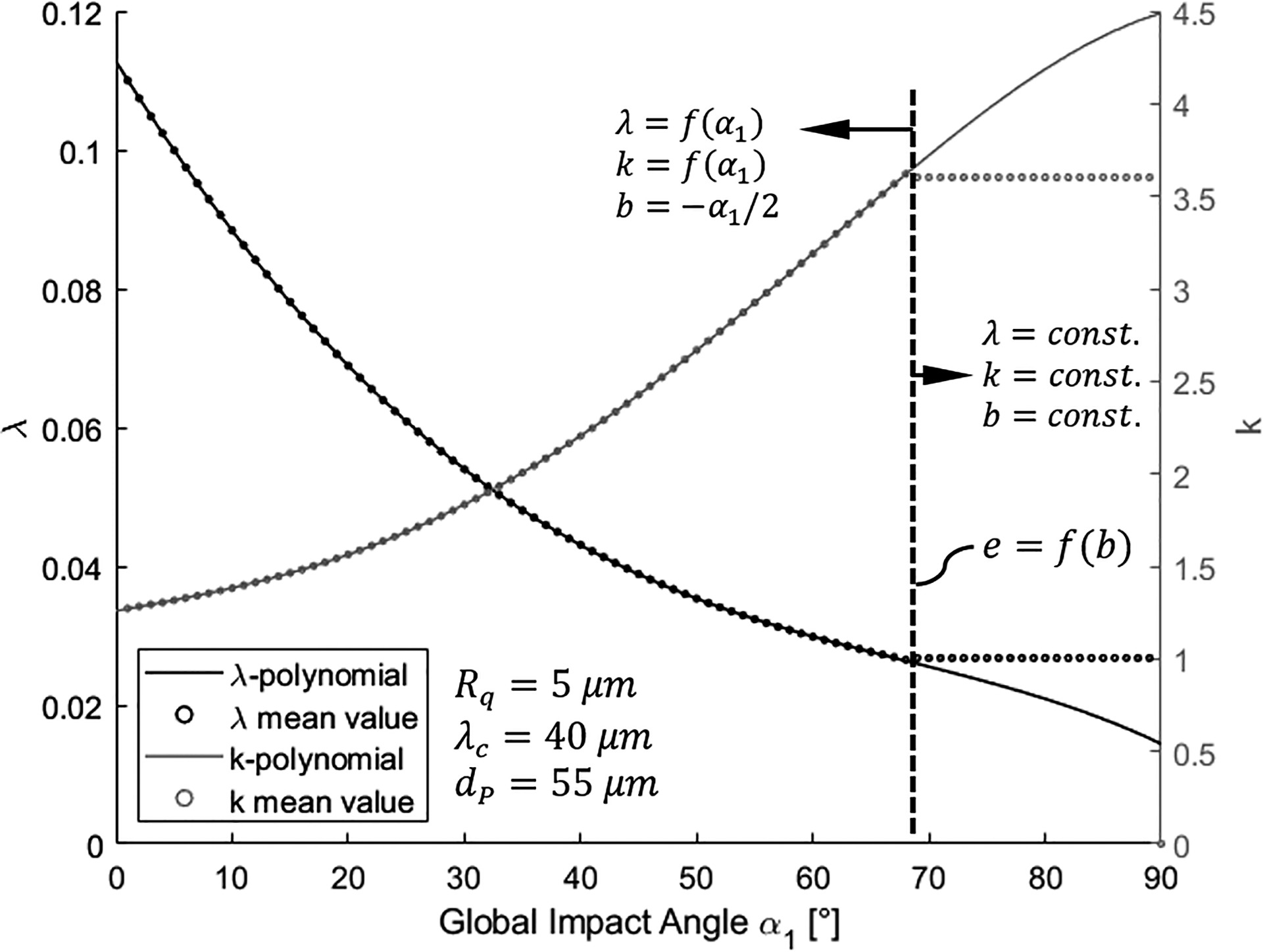
In the quest to predict the shifted distribution function with higher precision than the effective PDF by (Sommerfeld and Huber, 1999) but without the effort of additional iteration routines as proposed by (Konan et al., 2009). Two modelling strategies have proven to be promising:

1. Truncated Gaussian: A modified normal Gaussian PDF defined by

may be used for b≤Δα and P(γ;μ,σ,a,b)=0 for b>Δα and c<Δα (here c→+∞). In this context φ(x) is the probability density function of the standard normal distribution (σ2=1)

and ϕ(x) its cumulative distribution function

2. Alternatively the Weibull Distribution defined as

with k(α1)>0 as its shape parameter and λ(α1)>0 as its scale parameter might be used.

The truncated Gaussian approach can be determined by an analytical relationship from each slope angle distribution of the corresponding roughness profile. To use the Weibull distribution further pre-processing steps are necessary, because the parameters k and λ depend not only on the slope angle distribution but also on the global impact angle α1. In order to minimize the amount of memory required a polynomial approximation of forth degree is used for k(α1) and λ(α1) instead of storing these parameters for each combination of roughness, particle size and impact angle. As can be seen in Figure 7 the polynomial can only be used up to a boundary angle e. Above e the slope angle distribution is similar to a normal Gaussian distribution. For k=3.602 the Weibull distribution is in good approximation equal to the normal Gaussian. Hence the parameters can be treated as constant. In order to obtain stochastic significant mean coefficient the polynomial were determined for each combination of roughness and particle diameter from a sample of 100 simulations. In each simulation the probability density functions for all global impact angles (1–90 in 1 degree steps) were determined using the described routine for verification purposes by (Sommerfeld and Huber, 1999). Each is based on 100.000 samples, to assure a stochastic significant sample.

Figure 7.

Polynomial approximation for k(α₁) and λ(α₁).

In the current study, the database for the polynomial coefficients includes every combination in the course of the DoE. Constants exceeding the DoE can be determined by interpolation.

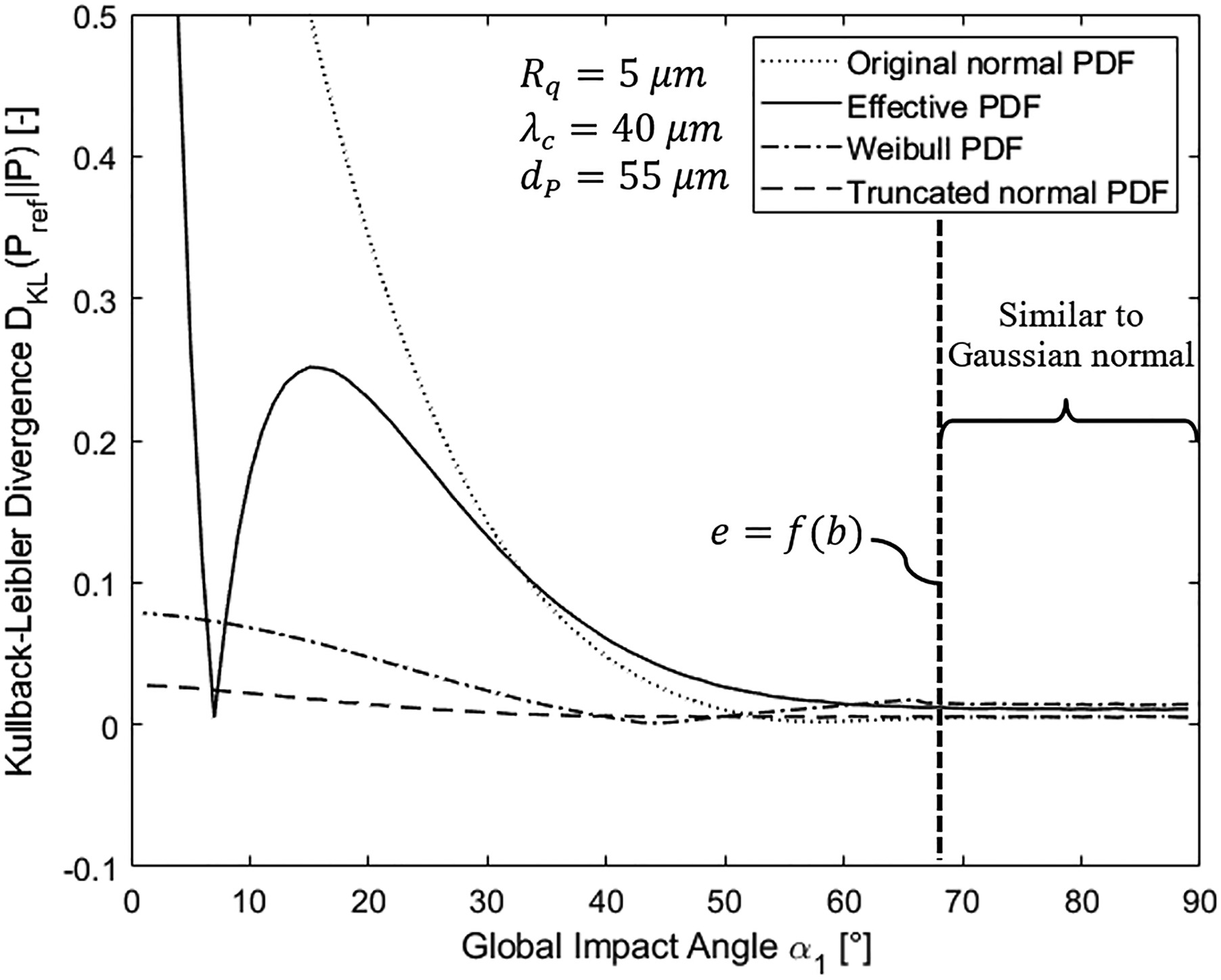
Choice of the PDF

In addition to the calculation of the coefficients the verification procedure by (Sommerfeld and Huber, 1999) enables the evaluation of the quality of the presented PDF's. The criterion to quantify the suitability is the previously described Kullback-Leibler divergence DKL. Figure 8 shows DKL for the different PDF's as a function of the global impact angle α1. Examples for the compared functions at three different α1 can be found in Figure 9. Obviously the effective normal distribution is quite well suited for large impact angles (DKL≪0.1). But for small impact angles it rapidly loses quality. Here the Weibull and the truncated normal distribution are far better suited. To decide between truncated Gaussian and Weibull distribution the decision has to be made whether a slightly better global agreement with the truncated distribution for all impact angles is preferred or a physically correct mapping of the boundary areas. The truncated normal distribution has the drawback of having a non-zero probability for a sliding rebound of particles. The Weibull distribution captures this effect having a zero probability for sliding on the wall. On the other hand, there is a slightly higher modelling effort for the Weibull distribution and a slightly higher DKL. In all subsequent examples the Weibull distribution is chosen, since physically correct modelling is desired, despite the more complex calculation.

Figure 8.

Kullback-Leibler Divergence D_KL over Global Impact Angle α₁.

Figure 9.

Additional inclination Δα for different global impact angles and R_q = 5 μm, λ_c = 40 μm, d_P = 55 μm.

Results and discussion

Based on roughness profiles which have been found to be characteristic for performance deterioration in compressor application (Bons et al., 2001) a sensitivity study has been conducted. A dimensionless roughness parameter ΦR was found that characterizes the effect of target surface roughness on statistical spread of rebound data. The roughness parameter is defined as:

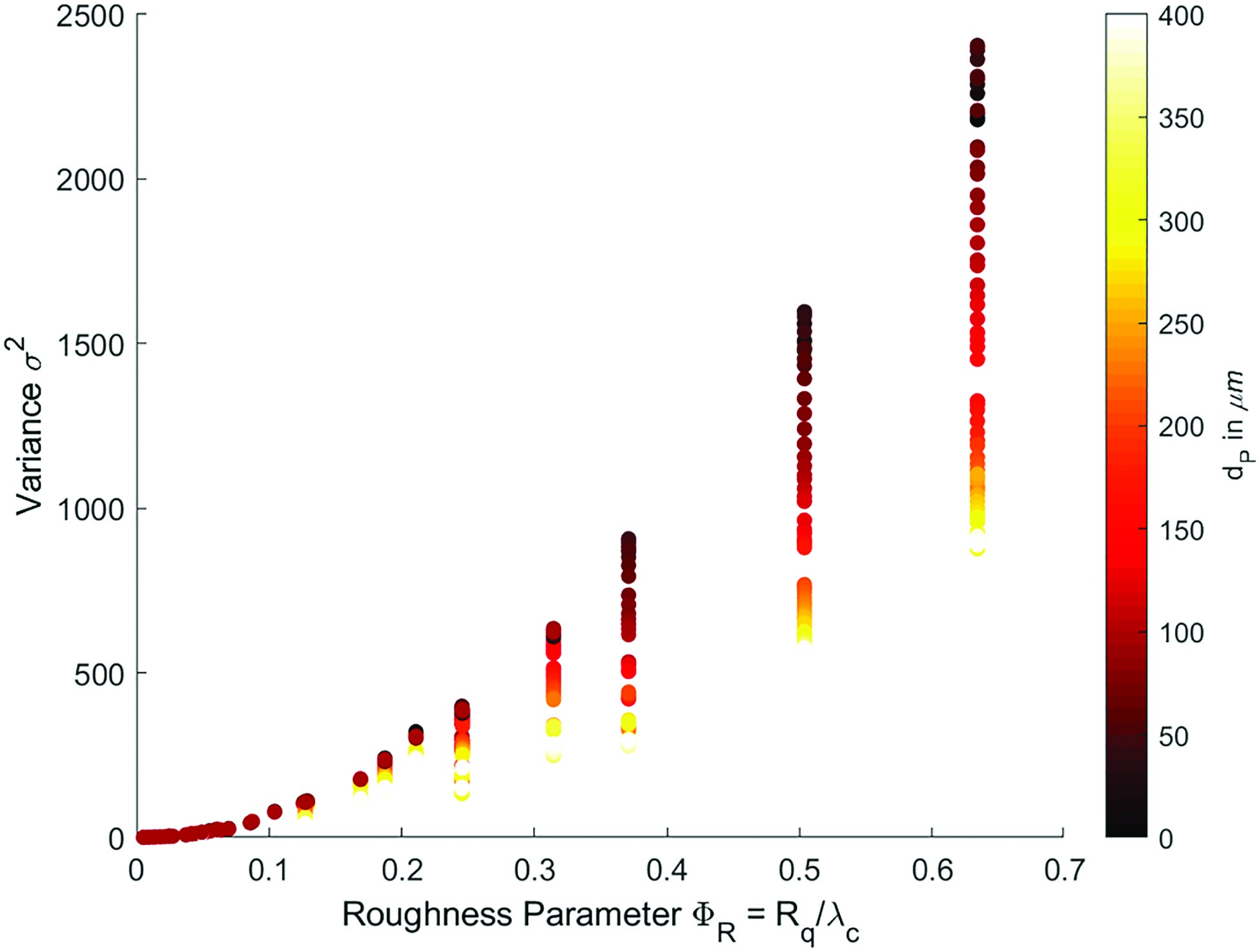
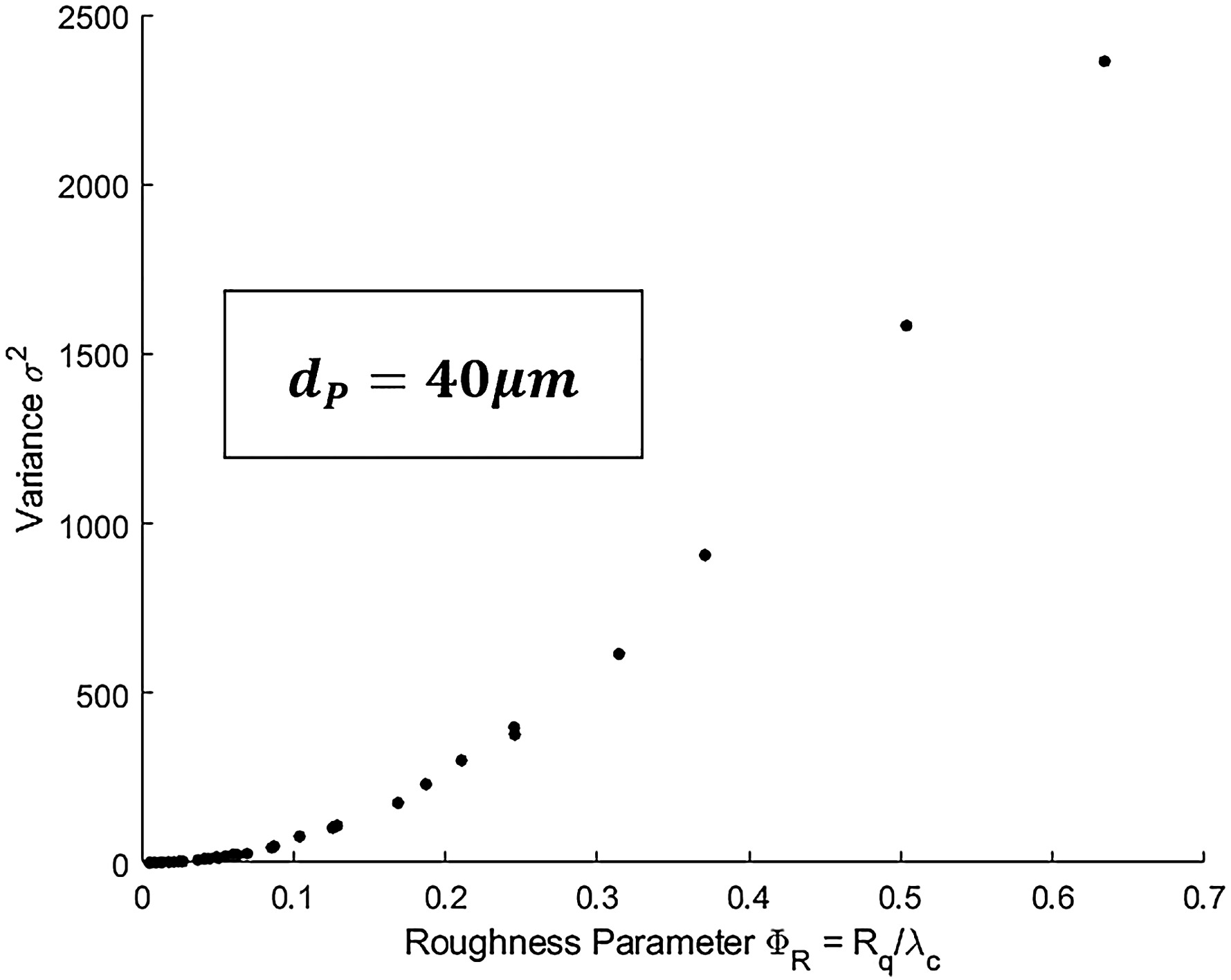
Figure 10 shows the variance of the additional inclination Δα over the roughness parameter ΦR for dP=40μm. Low values of ΦR correspond to small variations of the impact angles due to surface topography. Contrary higher values of ΦR indicate a significant deviation between local and global impact angle. Furthermore, with increasing ΦR not only the surface roughness as a single parameter but the combination of the surface topography and the particle size is significant for the variance of the inclination angle Δα (Figure 11). Hence for low values of ΦR(∼ΦR<0.1) the interaction of the particle size and ΦR can be neglected during numerical simulation for simplification purposes (σΔα2=f(ΦR)). For higher values of ΦR the variance need to be evaluated with respect to the combination of particle size and roughness topography (σΔα2=f(ΦR,dP)). Figure 12 shows this dependencies for the entire parameter range of the DoE.

Figure 10.

Variance of the additional inclination Δα over roughness parameter Φ_R.

Figure 11.

Variance of the additional inclination Δα over particle size d_p.

Figure 12.

Variance of the additional inclination Δα over roughness parameter Φ_R and particle size d_p.

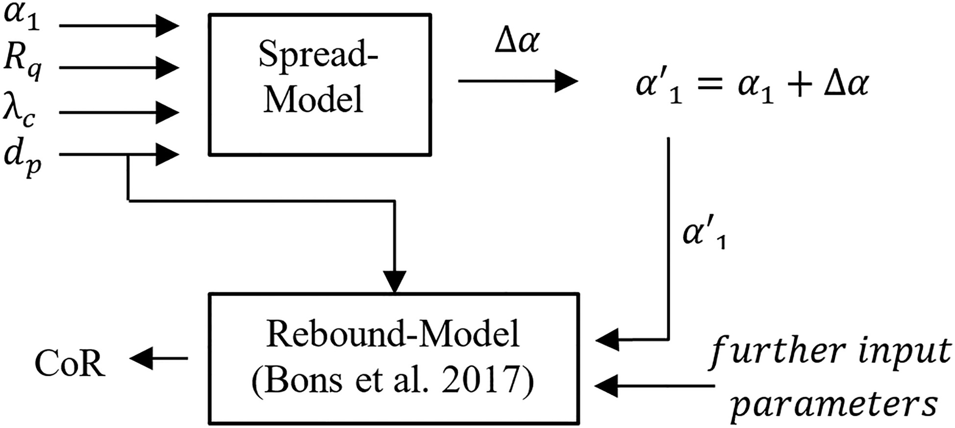
To evaluate the effect of the inclination angle on the statistical spread of the CoR, the developed Spread Model is connected with the Bons-Model (Bons et al., 2017) as shown schematically in Figure 2. In this process a random additional inclination angle Δα according to the probability distribution functions is generated with the principle of “inverse transform sampling” (Devroye, 1986). Let Δα be the desired parameter whose distribution can be expressed by the cumulative distribution function ΦΔα. The three subsequent steps are necessary:

The obtained random variable Δα fulfils the desired CDF ΦΔα and PDF. Applied to the Weibull distribution, the following dependency occurs:

This method allows to evaluate the statistical spread in CoR data due to the surface topography. Figures 13 and 14 show the synthesized CoR data for ΦR=0.04 and ΦR=0.13, respectively. For this calculation particle sizes range from 1 to 100 μm, with median value of dp=10μm. In addition the Bons-Model for dp=10μm is plotted as a reference. The theoretical variation of the surface topography leads to a significant spread in the synthesized CoR data, especially for high values of ΦR.

Figure 13.

Synthesized CoR data over the impact angle in comparison to the Bons-Model.

Figure 14.

Synthesized CoR data over the impact angle in comparison to the Bons-Model.

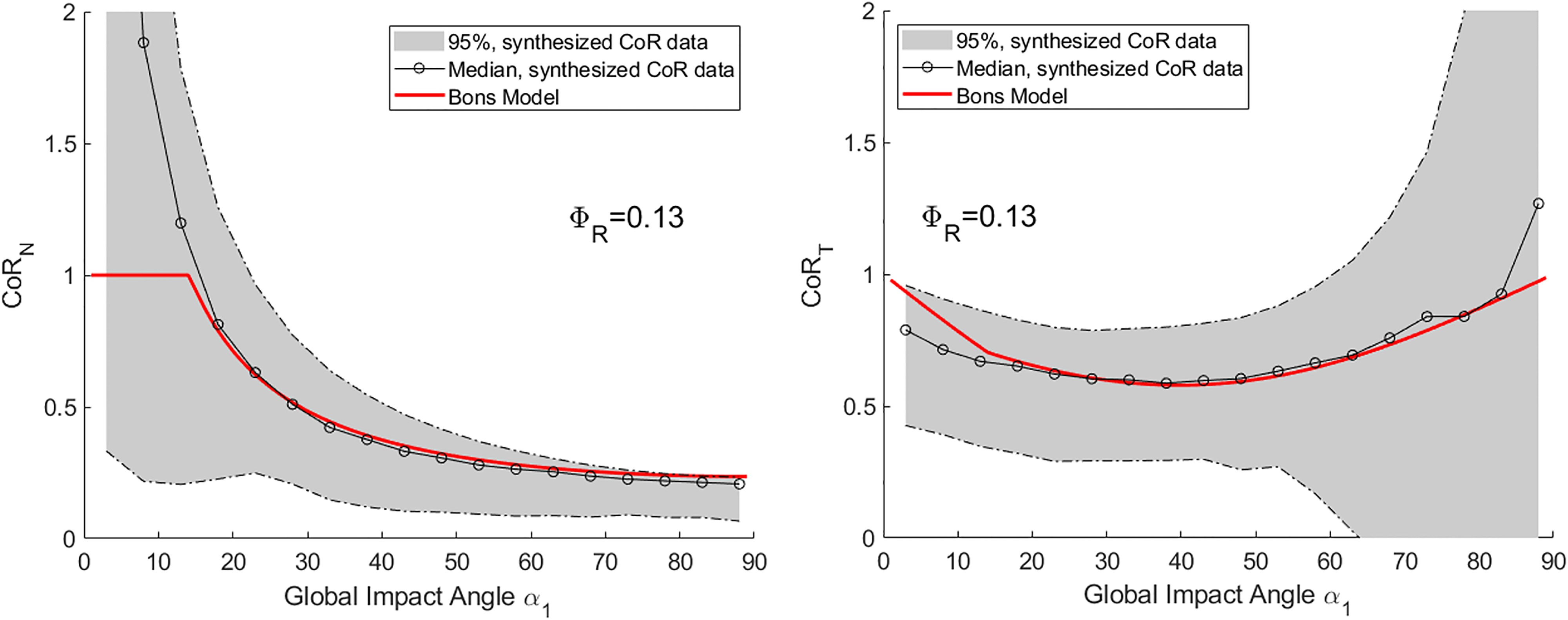
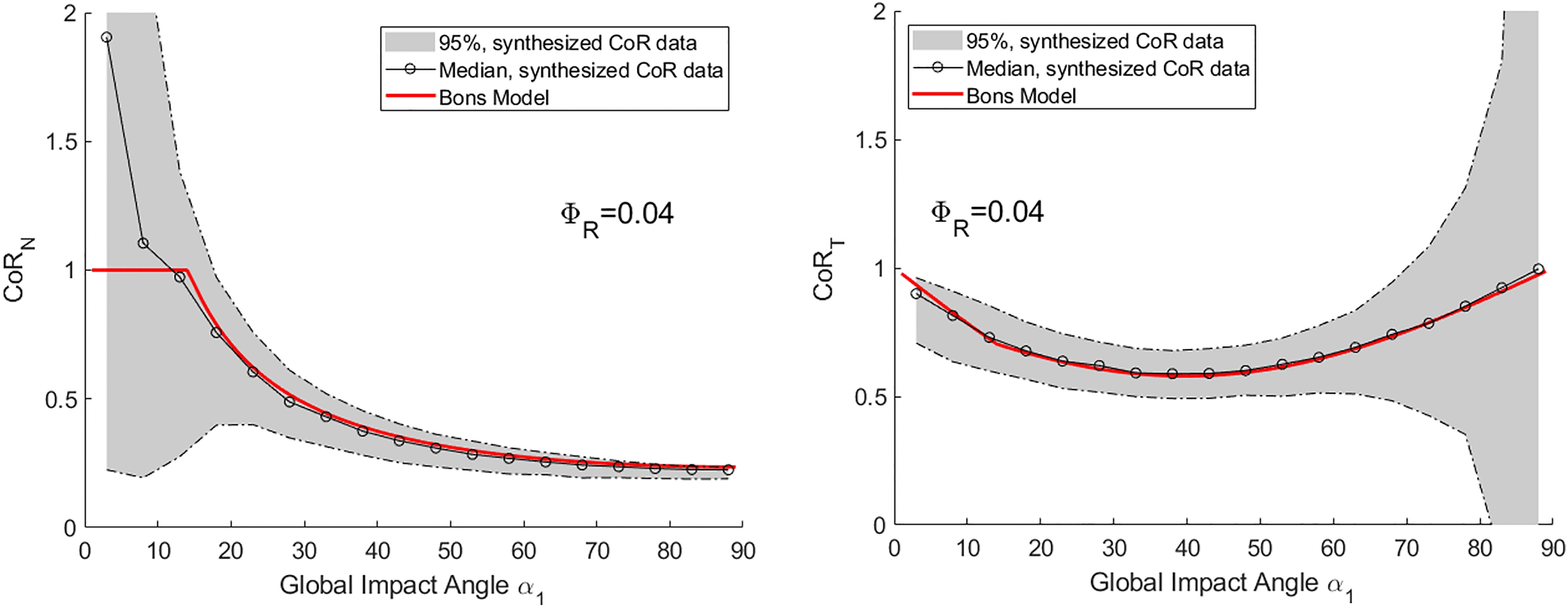
In order to analyse the observed data spread caused by surface roughness, the analytically generated data can be compared with experimentally obtained data from the literature – e.g. by Whitaker (Whitaker and Bons, 2018). The spread of synthesized data is in the same order of magnitude observed experimentally. This leads to the conclusion that the effect of surface roughness is significant for a particle's individual rebound behaviour and therefore must be taken into account in numerical simulations.

For the normal CoR the artificially generated data produce a scatter which is in good agreement with the measurement data by (Whitaker and Bons, 2018). The data spread is higher for small impact angles and decreases with rising angles. However the absolute value of the measurement data spread is under predicted for high global impact angles. For the tangential CoR the artificially generated data produce a scatter which is in good agreement with the spread in the data by (Whitaker and Bons, 2018) up to 80°.

Note that the measurement data by (Whitaker and Bons, 2018) as well as the presented model predict CoRN>1 for small impact angles. At low impact angles α1, the shadow effect leads to a high probability of a significantly positive Δα. The impacting particles are deflected at the rough surface and the high tangential component vT1 of the particle velocity is converted into a high normal fraction vN2 (Figure 15a). Therefore CoRN reaches values higher than unity. While the rise of normal CoR in the measured data by (Whitaker and Bons, 2018) is moderate, the shift in normal CoR values is significant higher in the prediction of the presented spread model. A similar effect can be observed for the tangential CoR for impact angles α1 close to 90°.

Figure 15.

Particle rebound for (a) small and (b) high global impact angles α₁.

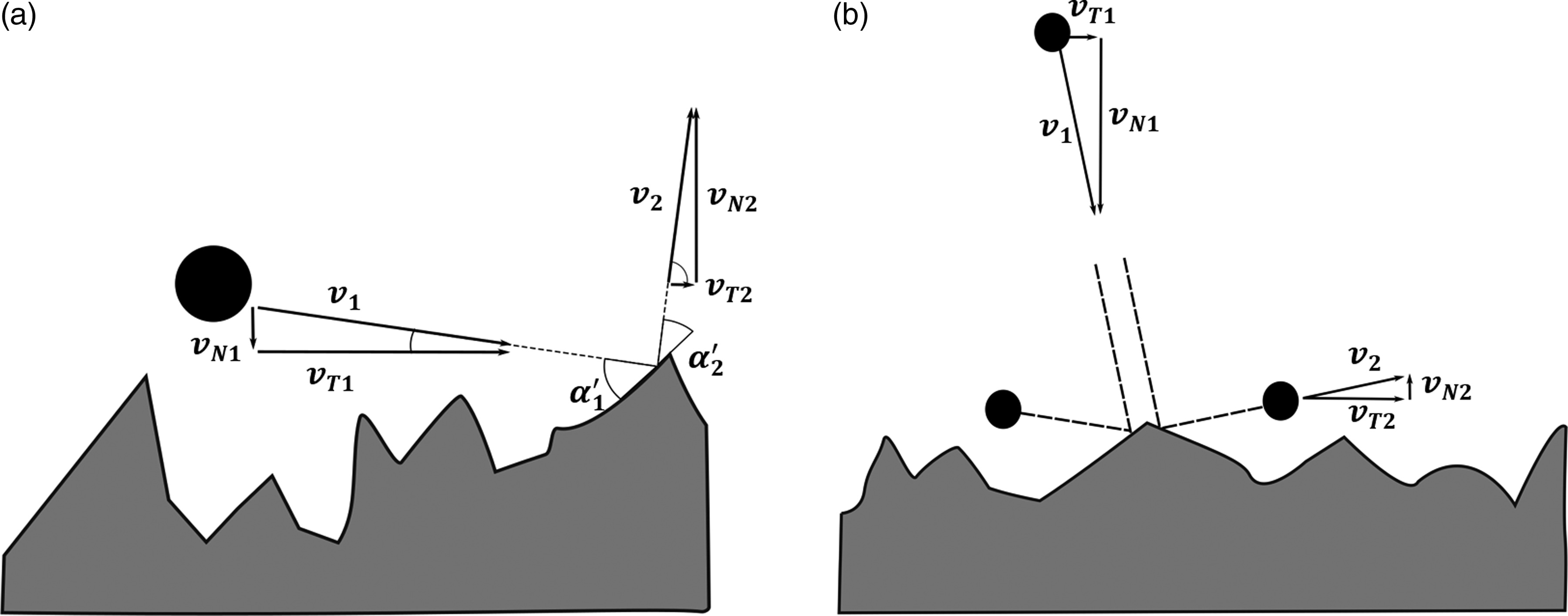
As can be seen in Figure 15b particles can be deflected in positive and negative direction, depending on the impact location. In addition the high normal velocity vN1 is converted into a high tangential fraction vT2. This effect was observed experimentally for positive tangential CoR. However the negative values of the tangential CoR are not observed in the experiment by Whitaker. This leads to the conclusion that in this region, other phenomena play a decisive role which superimpose the influence of roughness. The same applies to the discussion of the shift in normal CoR at small impact angles. Further phenomena like rolling and sliding of the particles, interaction with the surrounding fluid, or plastic deformation and erosion of the roughness peaks during contact and the associated dissipation of energy might superimpose the effect of surface roughness.

Investigation of these phenomena will be the aim of further research.

Conclusions

A spread model has been developed that estimates the statistical spread of rebound data due to target surface roughness through analytical considerations. It predicts the local impact angle of an individual particle by evaluating how deep a particle can theoretically penetrate the roughness profile with respect to its size. Based on roughness profiles which have been found to be characteristic for performance deterioration in compressor application a sensitivity study has been conducted. A dimensionless roughness parameter ΦR was found that characterizes the effect of target surface roughness on rebound spread data. Low values correspond to small deviation between local and global impact angle. Contrary higher values indicate a significant deviation. Furthermore, with increasing ΦR not only the surface roughness as a single parameter but the combination of the surface topography and the particle size is significant for the possible local impact angle variation that results in a spread of the coefficients of restitution. Connecting the possible variation of local impact angles with the Bons-Model induces a significant spread in the CoR-data. The spread of synthesized data is in the same order of magnitude observed by Whitaker (Whitaker and Bons, 2018) experimentally. This leads to the conclusion that the effect of surface roughness is significant for a particle's individual rebound behaviour and therefore should not be neglected in numerical simulations. This is especially relevant for increasing values of ΦR and decreasing particle sizes.

Nomenclature