Introduction
Steam turbines currently hold the largest share in the energy market, which highlights the importance of having robust and efficient machines. Recent advancements in steam turbines technology have led to increased area in the last stages of the turbines, with blade lengths reaching even 60 inches 08, in order to satisfy the need for higher power output. However, the design is quite challenging due to the fact that inlet flow conditions close to tip are supersonic in relative frame of reference. This leads to a generation of a bow shock wave upstream of the rotor’s leading edge 06 that, if not given sufficient space to decay, will interact with the upstream stator blade row, causing high flow unsteadiness or even potential boundary layer separation on the stator and increased kinetic energy losses 07.
Recent experimental measurements conducted in a low-pressure test facility of Mitsubishi Hitachi Power Systems, Ltd (MHPS) 02, confirm the presence of high unsteadiness in flow due to interaction of the travelling bow shock wave with the upstream stator but found no clear evidence of a boundary layer separation.
The goal of the current work is to investigate multistage effects and tip leakage flow in the last stage of the steam turbine. Before analysing these topics, however, an understanding is required of the unsteady interaction of the bow shock wave with its surroundings, i.e., the upstream stator blade row as well as the tip-cavity path of L-0 rotor and the leakage mass flow ingested in it.
In order to accomplish the objectives of this work, a computational domain has been set up consisting of the last two stages, L-1 and L-0 of the steam turbine. It is important to mention that focus is mainly given on analysing flow field of L-0 stage. However, the presence of L-1 is considered of high importance due to the fact that having the full unsteady flow field in the inlet of L-0 stage is generally more preferable than imposing circumferentially and time averaged boundary conditions, where all the flow features coming from outlet of L-1 stage are reduced to a single radial profile. Traces of L-1 stage’s leakage flow are identified in the inlet and outlet of L-0 stator.
Methodology
Geometry and computational domain
In this study, the last two stages (L-1 and L-0) of MHPS’s low-pressure (LP) steam turbine are considered. The geometrical model was created with a modified blade count for L-0 stators to allow the simulation of only a sector of the full annular domain and it includes full span shrouds and tip-cavity paths and seals for both rotor blade rows. However, the total number of blades in full annular was increased by only two blades, therefore the change is considered small enough for the flow field to remain representative of the original. Geometry is scaled by 1/3 to match the size of test turbine facility 03. Geometry solid surfaces and mesh were generated with the geometry of tip-cavities and seals of L-1 and L-0 rotors, as provided by MHPS, using AutoGrid5 and IGG meshing tools by NUMECA.
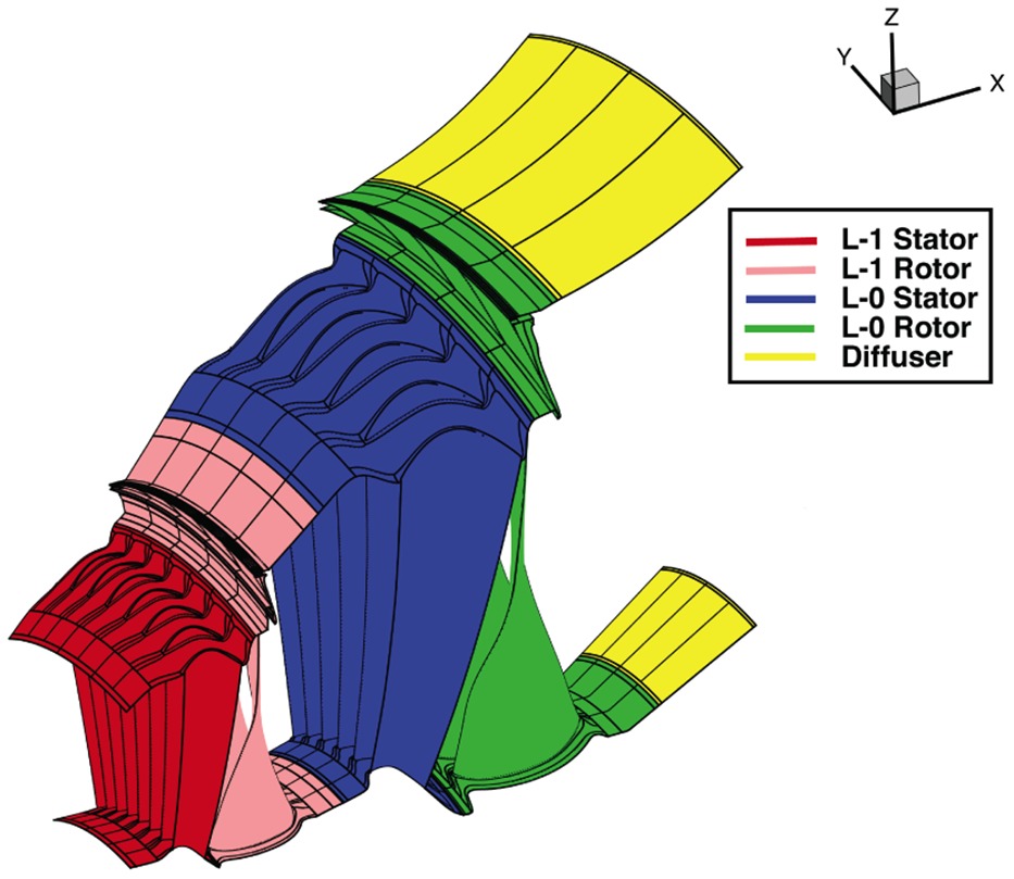
The computational domain consists of four blade rows plus the diffuser and is presented in Figure 1. A multi-block structured, body fitted mesh is generated for each passage separately. In total, 156 radial nodes were used in spanwise direction with higher clustering towards the endwalls. A larger portion of these nodes was clustered close to the tip-cavity regions of the rotors in order to increase the accuracy of the numerical model at the interaction zones of the cavity and the main flow. In total, 21 blades were modelled resulting in a mesh of almost 57 million nodes, of which more than 20 million were used in the regions of L-1 and L-0 cavities to resolve the complex geometry and capture unsteady flow features. The y+ value is kept below 2.5 in the whole computational domain. More details about the mesh of each blade row are given in Table 1.
Table 1.
Mesh size of the different flow domains.
| Domain | No. of blades | GPUs | Mesh size (millions) |
|---|---|---|---|
| L-1 stator | 7 | 3 | 9.2 |
| L-1 rotor | 5 | 5 | 21.8 |
| L-0 stator | 5 | 3 | 8.5 |
| L-0 rotor | 4 | 4 | 14.6 |
| Diffuser | - | 2 | 2.6 |
| Total | 21 | 17 | 56.7 |
The whole mesh was created with fully matching interfaces, both between blocks and row interfaces, in order to eliminate interpolation errors, which may lead to considerable loss of accuracy at the regions where highly unsteady phenomena take place.
Part-span connectors (PSCs)are not included in the numerical model, neither for L-1 nor for L-0 stage, due to the fact that including both them and the tip cavities and seals in the numerical model increase considerably the mesh generation complexity, as well as mesh size requirements. However, for the presented work, its effect is not significant as the analysis focuses above 90% of the radial span.
The full computational domain was split in 17 sub-domains in such a way to allow them to fit on-board GPU memory of six GBs of “Nvidia K20X” GPUs of Piz Daint computing system. 17 graphic cards were used in total. Simulations have been performed using in-house developed Computational Fluid Dynamics (CFD) code “MULTI3.” Recently, the solver was adapted to simulate equilibrium steam conditions. Detailed description of the solver is available in previous publication 01. Computational study has been carried out using Piz Daint Cray XC30 hybrid computing system in Swiss National Supercomputing Centre (CSCS) in Lugano, Switzerland.
Boundary conditions and simulation settings
The inlet boundary conditions are taken from experimental measurements conducted by MHPS at the exit of L-2 stage. The measurements have been performed at the inlet of the turbine and the outlet of each stage separately using a 5-hole probe (5HP), resulting in time-averaged radial profiles of flow quantities. Using these experimental data, non-uniform, radial profiles of total pressure and total temperature, along with flow angles (yaw and pitch) distributions are imposed in the inlet of the computational domain.
Regarding outlet boundary conditions, representative value of static pressure, also extracted from experimental measurements, with radial equilibrium is imposed at the hub endwall in the diffuser outlet. The sliding interface approach is used at the interface between the rows. Unsteady simulations have been performed, under these boundary conditions, using dual time stepping approach.
Due to the presence of very fine cells in the computational mesh, especially close to the cavity regions, a sufficient number of sub-iterations is needed in order to ensure proper propagation of information through the regions of very high node clustering, due to the fact that smaller cells need more sub-iterations for the flow to develop properly compared to bigger cells. 120 equal time steps have been used for each period, with 200 sub-iterations per time step. Both numbers are a result of a separate study that was conducted during the course of the main investigation.
The simulation has covered more than three-full revolutions of the rotor domain. One full rotor revolution requires 4.5 days for completion. By the end of the simulation, an unsteady periodic solution has been achieved and the calculated mass flow rate in the inlet of the domain shows a difference below 0.4% compared to the one experimentally measured.
Results and discussion
Validation of numerical model
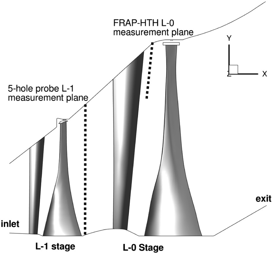
The validity of the numerical model has been extensively evaluated with available experimental measurements conducted in the test facility. More specifically, predictions of the CFD model have been compared with 5HP measurements conducted by MHPS at the outlet of L-1 and L-0 stages. More importantly, numerical results were additionally compared with time resolved and time averaged measurements at the stator exit of the last stage of MHPS’s LP steam turbine that were conducted 02. Measurements were conducted in MHPS’s test facility in Japan using a novel fast response heated probe (FRAP-HTH) and was the first time that time resolved measurements in wet steam environment with supersonic relative flows at the rotor inlet had ever been reported. Details on FRAP measurement method and uncertainty are available in the original publication 02.
The locations of the experimental measurements that were used for comparison with the current numerical study are presented in Figure 2.
Comparison of CFD with 5-hole probe at L-1 rotor exit
Figure 3 and Figure 3 show comparison of CFD with 5HP experimental data for absolute yaw angle, as well as total temperature across the blade span at L-1 rotor exit, respectively.
Figure 3.
Comparison of CFD and 5HP for absolute yaw angle (a) and total temperature (b) at rotor exit of L-1 stage.
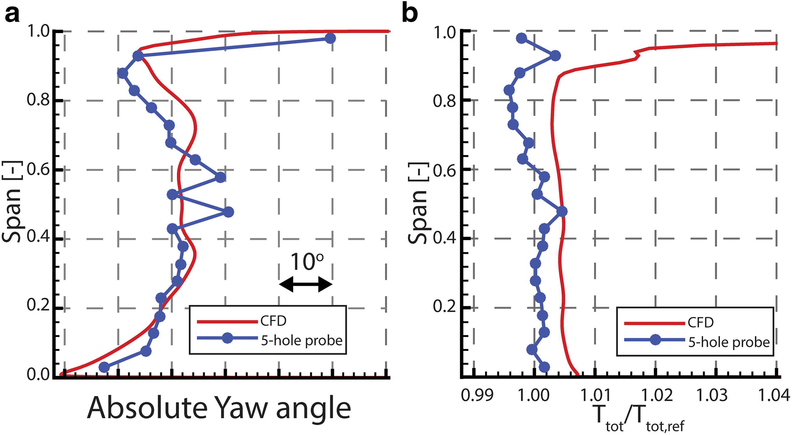
CFD results are circumferentially averaged over five rotor pitches and time averaged over five rotor blade passing periods of L-1 rotor blades with 156 nodes in spanwise direction, while 5HP measurements were performed along a single radial traverse and averaged over 10 sample data measured at intervals of a second with 20 points in spanwise direction.
For confidentiality reasons, only grid resolution is shown for absolute yaw angle, while total temperature has been normalised by dividing both numerical and experimental data with the mean of experimental values.
As shown, a good agreement has been achieved between numerical results and experimental data, both in trends and absolute values across the span. The root mean square (RMS) deviation between them is 3.8° but the value is increased due to the very high gradient close to the tip. The mismatch in yaw angle between 40% and 60% of the span is due to the presence of the PSC, which causes an overturning of the flow at 58% and 48% span. PSCs are not included in the numerical model.
Total temperature is well predicted by CFD, with RMS difference from experiments equal to 1.15%. The effect of PSC is also visible on total temperature that causes a slight increase in the exact same span locations.
It is worth noting here that total temperature is not calculated using isentropic relations of the ideal gas but is rather indexed directly from the steam tables.
Comparison of CFD with time-averaged FRAP-HTH probe at L-0 stator exit
In this paragraph, CFD predictions are compared with time-averaged results of FRAP-HTH measurements at the outlet of L-0 stator. This area is of particular interest because the flow becomes supersonic in the relative frame of reference in the inlet of the last rotor, generating a shock wave upstream of the rotor leading edge 07. Figure 4 and Figure 4 show comparison of CFD with FRAP-HTH for delta flow yaw angle and relative Mach number, respectively.
Figure 4.
Comparison of CFD and time-averaged FRAP-HTH for delta flow yaw angle from the mean blade metal angle (a) and relative Mach number (b) at L-0 stator exit.

In Figure 4 the absolute yaw angle is subtracted from the mean blade metal angle, representing essentially the deviation flow angle at the stator blade exit. Positive values indicate overturning of the flow, while negative values imply flow underturning. In Figure 4, relative Mach number has been normalised by dividing both numerical and experimental data with the mean of experimental values.
CFD results in Figure 4 are circumferentially averaged over five L-0 stator pitches and time averaged over four rotor blade passing periods of L-0 rotor blades with 57 nodes in spanwise direction, while FRAP-HTH measurements are time averaged and circumferentially area averaged over one L-0 stator pitch with 16 points in spanwise direction.
Comparison shows that yaw angle is slightly over predicted by 2.4° on average compared to measurements but trend is captured accurately. The reason of the mismatch could rely on the fact that the computational model has a slightly modified blade count compared to the real, which was done in order to allow the simulation of only a sector of the full annulus. The offset could also be due to probe alignment error during installation.
Relative Mach number also matches well the measurements both in trend and in absolute values, with RMS deviation equal to 3.27%. The difference observed above 90% span could be due to the fact that measured values are very close to the probe’s calibration range.
Comparison of CFD with time-resolved FRAP-HTH probe at L-0 stator exit
Comparison of CFD predictions with time-averaged FRAP-HTH and 5HP experimental data has shown good agreement. Finally, numerical prediction of static pressure coefficient, Cps, at 90% span at the exit of L-0 stator is compared with time-resolved experimental data of FRAP-HTH and results are presented in Figure 5, for four time steps of one rotor blade passing period. Direction of rotation is from left to right and observer looks downstream in all figures.
Figure 5.
Comparison of CFD and time-resolved FRAP-HTH of Cps [-] at L-0 stator exit, 90% span — Unsteady comparison in four time steps of one rotor blade passing period.
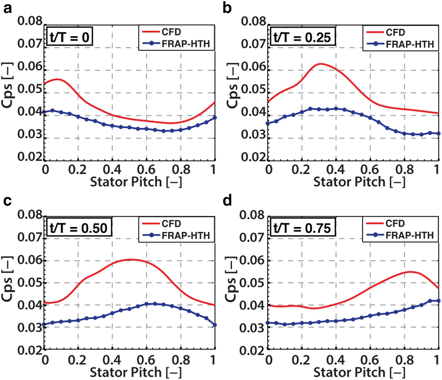
Static pressure coefficient is defined in . It is important to mention that the inlet refers to the conditions in the inlet of the machine, not the inlet of the computational domain. Exit refers to the conditions in the exit of the machine.
As shown in Figure 5, there is a good agreement between CFD and experiments, both in trend and phase of the unsteady peak-to-peak fluctuations for all time steps. The difference in absolute values is probably due to the different spatial resolution of the two methods. Regarding the experimental results, the FRAP-HTH probe tip size enables a minimum spatial resolution of 2.5 mm in the circumferential direction where the shock propagates. This poses limitations in spatially resolving the pressure step of the shock wave due to the greater tip size compared to the shock wave length scale 05. On the other hand, the greater spatial resolution obtained with the CFD results, with maximum cell distance of 0.95 mm, result in higher peak-to-peak fluctuations of the static pressure coefficient and it is believed that this is the main reason for the difference in absolute values. The interaction of the shock wave with the probe requires further investigation.
The results presented so far show that the modified solver with equilibrium steam modelling is able to provide reliable predictions of the flow field in the last two stages of the LP steam turbine. Being able to trust CFD predictions is crucial in understanding the complex, unsteady, three-dimensional flow features in wet steam flows and in gaining insight of the flow in regions were measurements are infeasible.
Unsteady bow shock wave interaction with stator
As it has been reported 02, the detached bow shock wave at the rotor leading edge of the last stage increases the flow unsteadiness compared to the subsonic region, both in pressure and flow angles. Supersonic airfoils require unique incidence in the inlet 07 and this increased unsteadiness can lead to higher losses. Key in identifying the cause of this is to understand the stator-rotor interaction and its effect on the flow field. For this reason, time resolved results are presented in this section.
Figure 6 presents blade-to-blade contours of static pressure coefficient at 90% of the blade span, where the flow is supersonic relative to the rotor inlet, in six time steps of one rotor blade-passing period.
Figure 6.
Static pressure coefficient Cps [-] at 90% span — Bow shock formation and interaction with upstream stator for one rotor blade passing period.
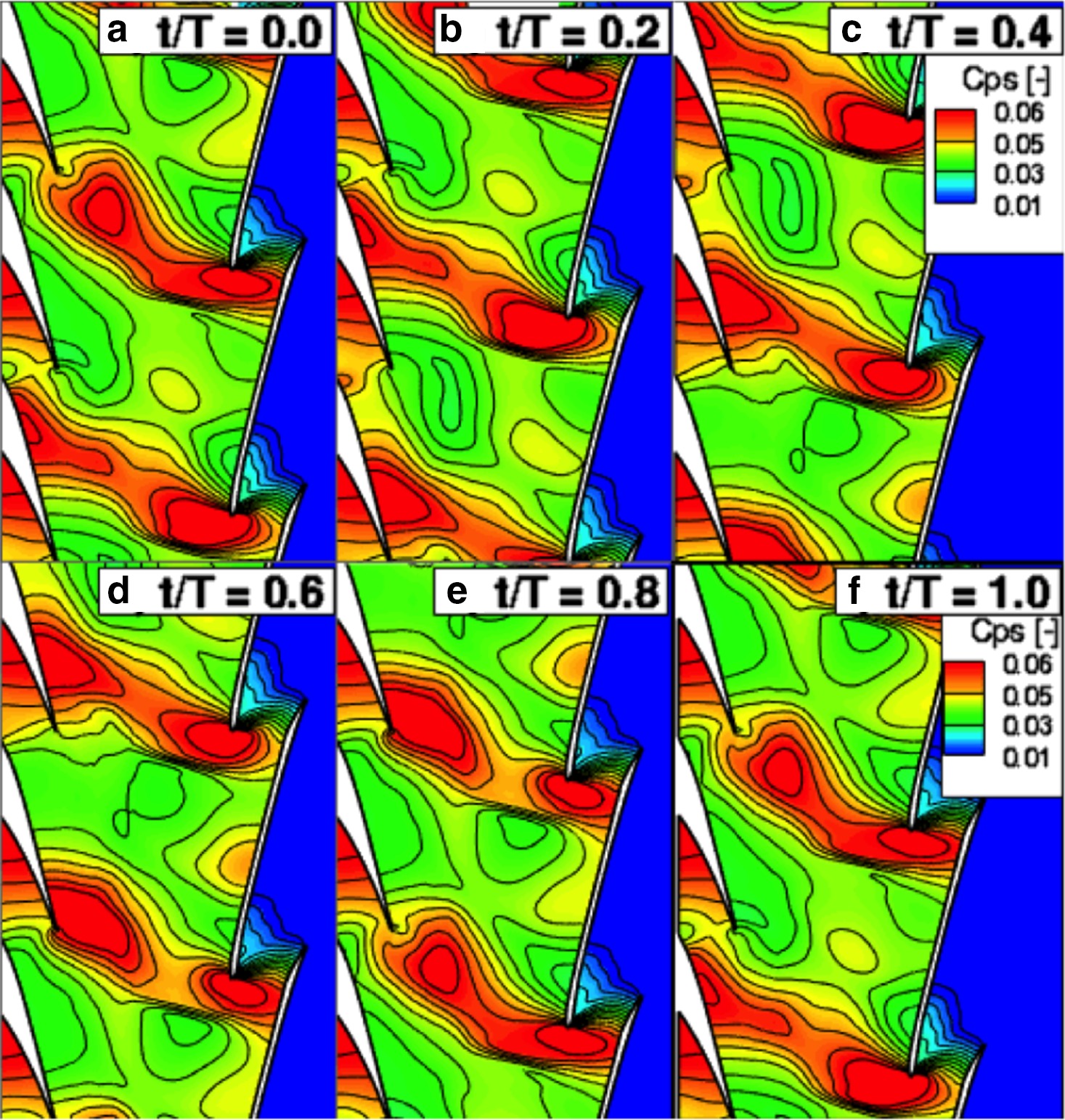
Direction of flow is from left to right and the rotor blades are moving from top to bottom. The bow shock wave can be identified by regions of sharp increase of static pressure or Cps values. Analysis will focus on the trailing edge of the second stator blade looking from the top.
In the beginning of the period, the bow shock wave is not interacting with the suction side of the upstream stator, as seen in Figure 6. As the rotor blades are moving, the bow shock wave impinges on the suction side of the upstream stator and starts moving along it (Figure 6 and Figure 6). It is observed that the boundaries of high-pressure region caused by the bow shock wave are fairly straight, as shown by the black dashed lines in Figure 6. However, as it is moving with the rotor blade, it starts interacting with the stator trailing edge and its shape deforms and bends backwards, opposite to the direction of rotation (Figure 6). While it tries to overcome the trailing edge, it can be seen that static pressure is increasing also in the pressure side of the upstream stator. Finally, the shock detaches from the trailing edge of upstream stator and impinges on the suction side of the next upstream stator blade, Figure 6.
In order to further analyse the effect of the bow shock wave interaction with the upstream stator, the unsteady flow field was investigated for a single stator pitch at two axial locations, at 92.5% and 107.5% of the blade’s axial chord. The locations are visible in the schematic in the top of Figure 7 and side of Figure 9, respectively. The results are presented in Figure 7 to Figure 10 and the observer looks downstream in all figures.
Figure 10.
Circumferential distribution of Cps [-] at 107.5% axial chord of L-0 stator blade, 90% span.
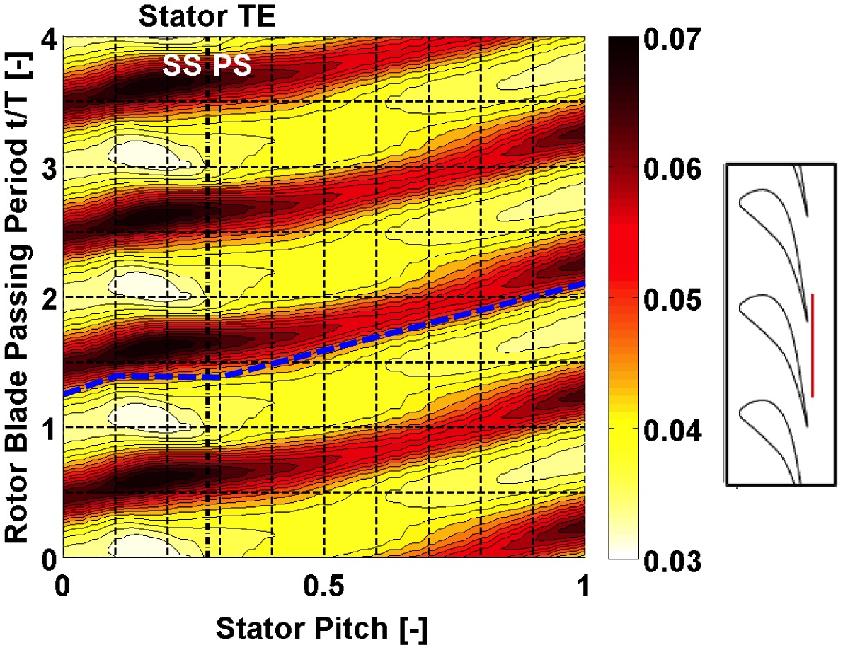
Figure 9.
Circumferential distribution of deviation flow angle [o] at 107.5% axial chord of L-0 stator blade, 90% span.
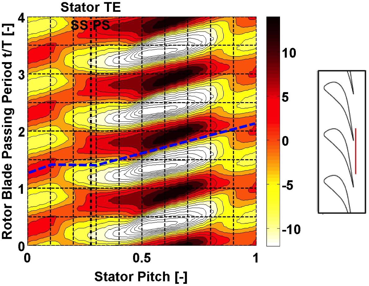
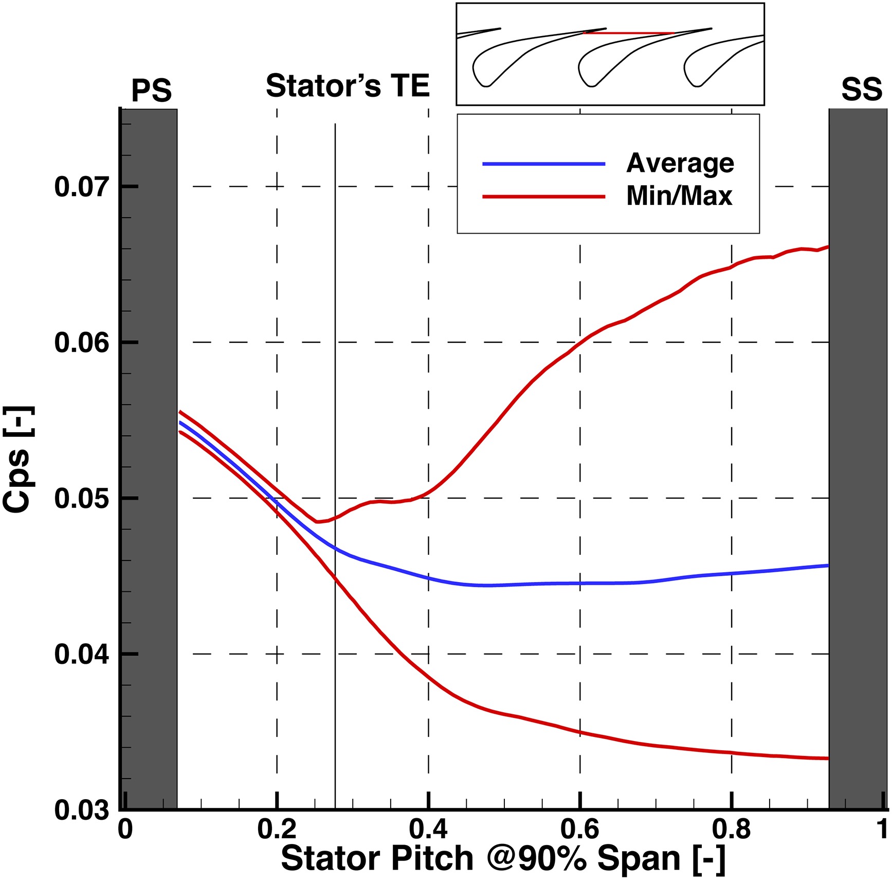
Figure 7 shows the circumferential distribution of static pressure coefficient at the passage between two blades at 90% span, located at 92.5% of stator’s axial chord. The results are time averaged over four rotor blade passing periods and are presented with the solid blue line, for one stator pitch. The solid red lines represent the minimum and maximum values of all time steps, obtained from the unsteady data. Since the axial line cuts through the blades, approximately 7% from left and right in the plot represent the pressure side (PS) and suction side (SS), respectively, with the grey shaded area.
As shown in the Figure 7, starting from the pressure side, the time averaged static pressure coefficient decreases from 0.055 to 0.045 at around 40% of stator pitch and remains constant along the stator pitch until the suction side. The peak-to-peak fluctuations are relatively low in the region close to the pressure side and increase almost 24 times close to the suction side, where they reach ±34.4%. The interaction of the bow shock wave with the flow in the unguided region above 30% of the stator pitch is very clear by the high unsteadiness present, while the flow shows very low unsteadiness below 30% because it is protected from the influence of the shock wave by the downstream part of the solid blade. For the calculation of the peak-to-peak fluctuations, was used.
It is additionally observed that the maximum Cps on the suction side is greater than the maximum Cps on the pressure side. This implies that there are moments in time when the blade is counter-loaded close to the trailing edge of the blade.
These high fluctuations on static pressure not only increase the unsteady loading in the blade but, in worst case could even lead to a boundary layer separation on the suction side of the blade, which would be detrimental for the efficiency. If there were a boundary layer separation, one would expect that the axial velocity would receive negative values due to flow recirculation. However, looking at the axial velocity in Figure 8, there is no such evidence of a boundary layer separation.
Figure 8.
Circumferential distribution of normalized axial velocity Cax [%] at 92.5% axial chord of L-0 stator blade.
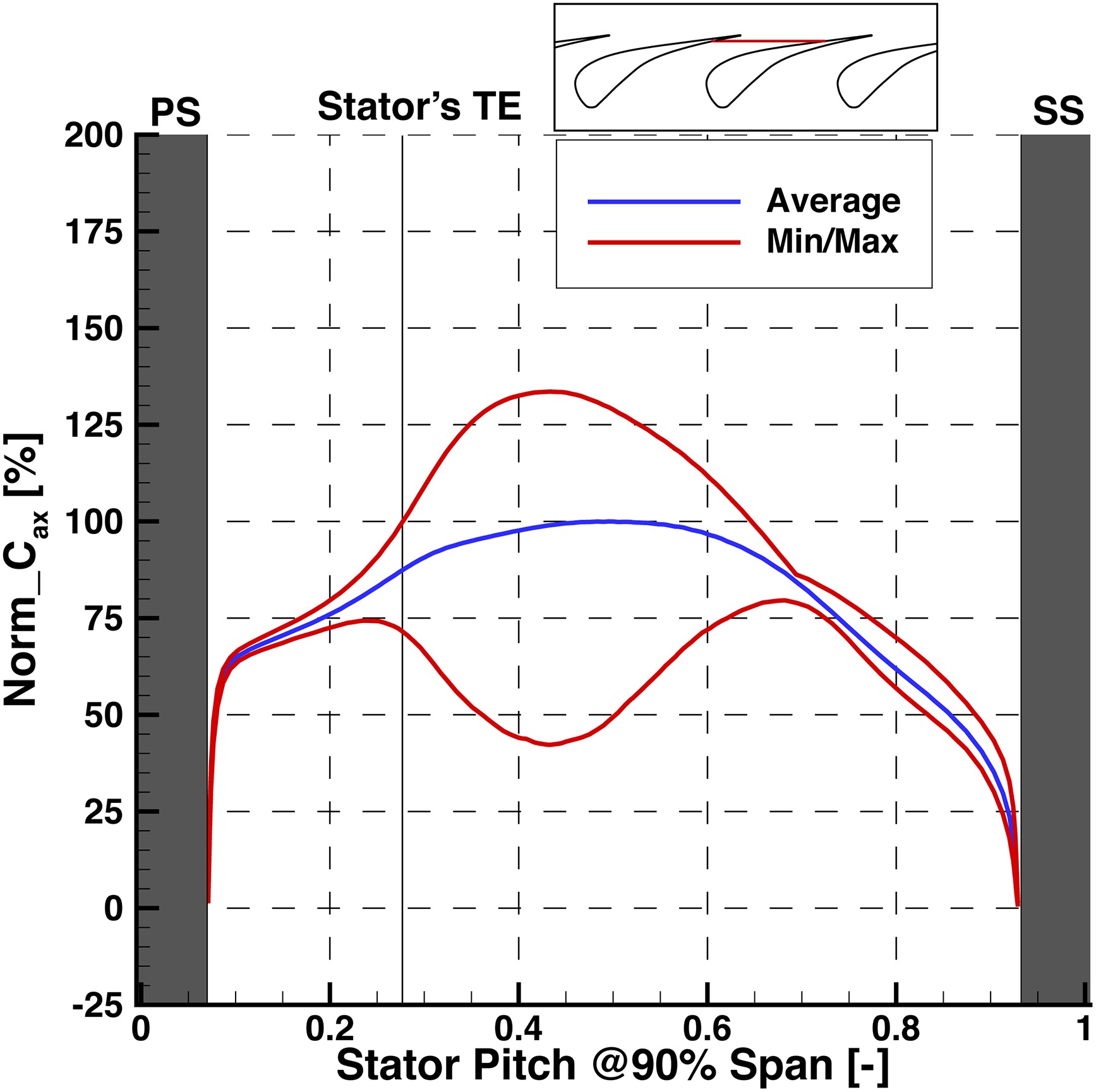
The axial velocity is reducing to zero close to the walls due to the no-slip boundary conditions. Both time averaged and min-max values have been normalised with the maximum velocity of the time averaged results, located in the centre of the passage. As seen in Figure 8, unsteadiness is fairly low close to the pressure side of the blade with ±4.5% fluctuations, while it is more than double close to the suction side with ±10.4% peak-to-peak variations. More importantly, the line of minimum Cax is greater than zero at all time steps, implying there is no flow recirculation at any point in time due to the interaction with the travelling shock wave. This confirms previous findings 02, where no clear evidence of periodical wake widening could be experimentally measured.
To analyse the flow field downstream of stator, time-space diagrams for four-rotor blade passing periods are used for one stator pitch at 107.5% of axial chord and 90% span. Figure 9 and Figure 10 show the absolute flow yaw angle relative to the blade metal exit angle (deviation angle) and the static pressure coefficient Cps, respectively. Positive values of deviation angle indicate flow overturning while negative values imply flow underturning. Location of the line is shown on schematic at left of the figures.
In both plots, features travelling with the downstream rotor appear as inclined parallel lines (i.e., bow shock wave), while features related to the stationary frame of reference are visible on vertical lines (i.e., stator wake). Observer looks downstream in both plots.
The time-averaged results of deviation angle have shown a constant underturning along the whole stator pitch of 2.5° on average, while the unsteadiness is ±3.1° at 20% of the pitch. The high fluctuations observed in the middle of the passage between 30% and 70%, both in Figure 8 and Figure 9 are related to the modulation of the wake due to the interaction with the passing shock wave. Both axial locations of 92.5% and 107.5% happen to capture the upstream and downstream boundary, respectively, in which the modulation of the wake occurs.
As seen on Figure 9, the minimum and maximum values appear in constant position but also have a smeared shape. This is because, as the shock wave overpasses the trailing edge of the stator, it interacts with the incoming wake, overturning the flow. As the shock wave moves further, static pressure drops because the flow has enough space to expand, leading to an underturning in that region.
As observed in Figure 10 the shock wave has its highest intensity when located close to the stator trailing edge due to available area reduction, and is reduced again afterwards since it has more axial distance from upstream stator, which allows it to weaken slightly. It is also interesting to notice, that the inclined shape of the shock wave flattens at around 10% of the passage and is inclined again after 30%. This is because the shock wave is bending backwards and interacts with the trailing edge for longer time, as it has been explained on Figure 6.
Effect of axial distance of L-0 rotor leading edge from upstream stator on the shock intensity
It was shown previously in Figure 10 that the shock wave has its lowest intensity when it overpasses the upstream stator’s trailing edge and has enough space to decay. In a previous computational study 09, the rotating shock wave weakens before it reaches the stator, showing a very steady behaviour. However, increasing the axial distance between stator and rotor in an existing machine would be a challenge due to limitations coming from bearing locations. Potential solution would be to apply forward sweep on the stator, close to the tip. This would not only increase the stator-rotor gap, but could also help with the reaction variation and the rotor work variation 04.
Since there was no geometry available with larger stator-rotor gap, in order to further investigate the effect of axial distance of the L-0 leading from the upstream stator, the unsteady flow was analysed on a line along the suction side of the stator for four rotor blade passing periods, at 90% span, since the axial distance of the rotor leading edge from the suction side of the stator varies in time between 2.36 and 3 rotor blade axial chords, at 90% span.
Figure 11 shows the distribution of static pressure coefficient along the line close the suction side for four rotor blade passing periods, ranging from 77.5% until 105% of the stator’s axial chord, where 100% is the trailing edge of the stator. The location of the line is shown on schematic of Figure 12.
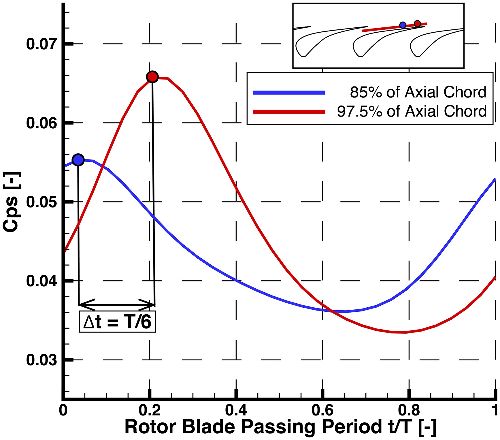
Figure 11.
Cps [-] distribution along stator suction side between 76% and 105% of stator axial chord, at 90% span.
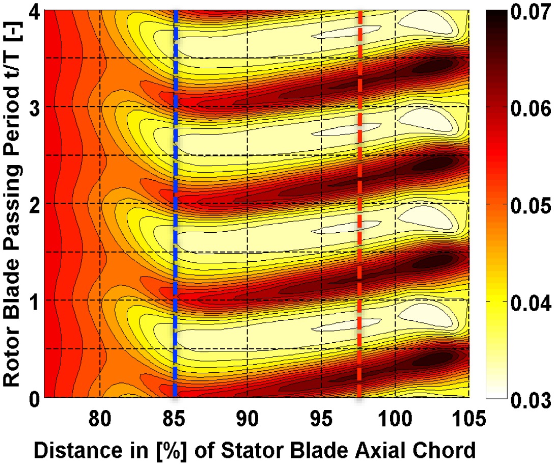
As seen in Figure 11, the flow shows low unsteadiness in time up to approximately 80% of the axial chord. The flow further of 83% is unguided and the unsteadiness increases due to the interaction with the travelling shock wave. This axial location coincides with the throat of the passage.
It is also observed that the maximum Cps has a decreasing trend further from the trailing edge, implying that the intensity of the shock wave is weakening. However, the blade does not experience the maximum loading at each axial location at the same time step. In order to verify and analyse further, Cps at two axial locations, at 85% and 92.5% of axial chord, is shown in Figure 12 for one rotor blade passing period.
As seen in Figure 12, the maximum Cps decreases as the shock wave impinges further from the trailing edge, by 15.7%. It is clear that larger stator-rotor gaps are desirable in order to decrease the unsteadiness due to the stator-rotor interaction. What is more important is that the maximum at these two locations have a difference in phase equal to one-sixth of the rotor blade passing frequency. This is of high importance because these high fluctuations on the unsteady loading of the blade, along with the difference in phase between the axial distance, could potentially lead to high cycle fatigue or failure and needs to be taken into account during the design process.
Unsteady bow shock wave interaction with L-0 rotor cavity path
Analysis of the full flow field has shown that the bow shock wave upstream of the leading edge of the last stage’s rotor is a highly three-dimensional feature. As the radius of the machine increases, so does the travelling speed of the blades, leading to an increase of relative inlet Mach number. It has been seen that the shock wave that is formed is impinging on the casing, interacting with the shroud of the blade and the inlet to the tip-cavity path. Shrouds in such long blades are crucial both to reduce the losses from tip leakage flows, as well as to ensure the mechanical integrity of the long blades. The leakage flow that goes through the cavity path does not produce any power on the rotor, therefore it is desirable to quantify this amount of flow. In this section, the flow field in the inlet of the tip cavity is analysed in order to quantify the leakage flow and assess the interaction with travelling shock wave.
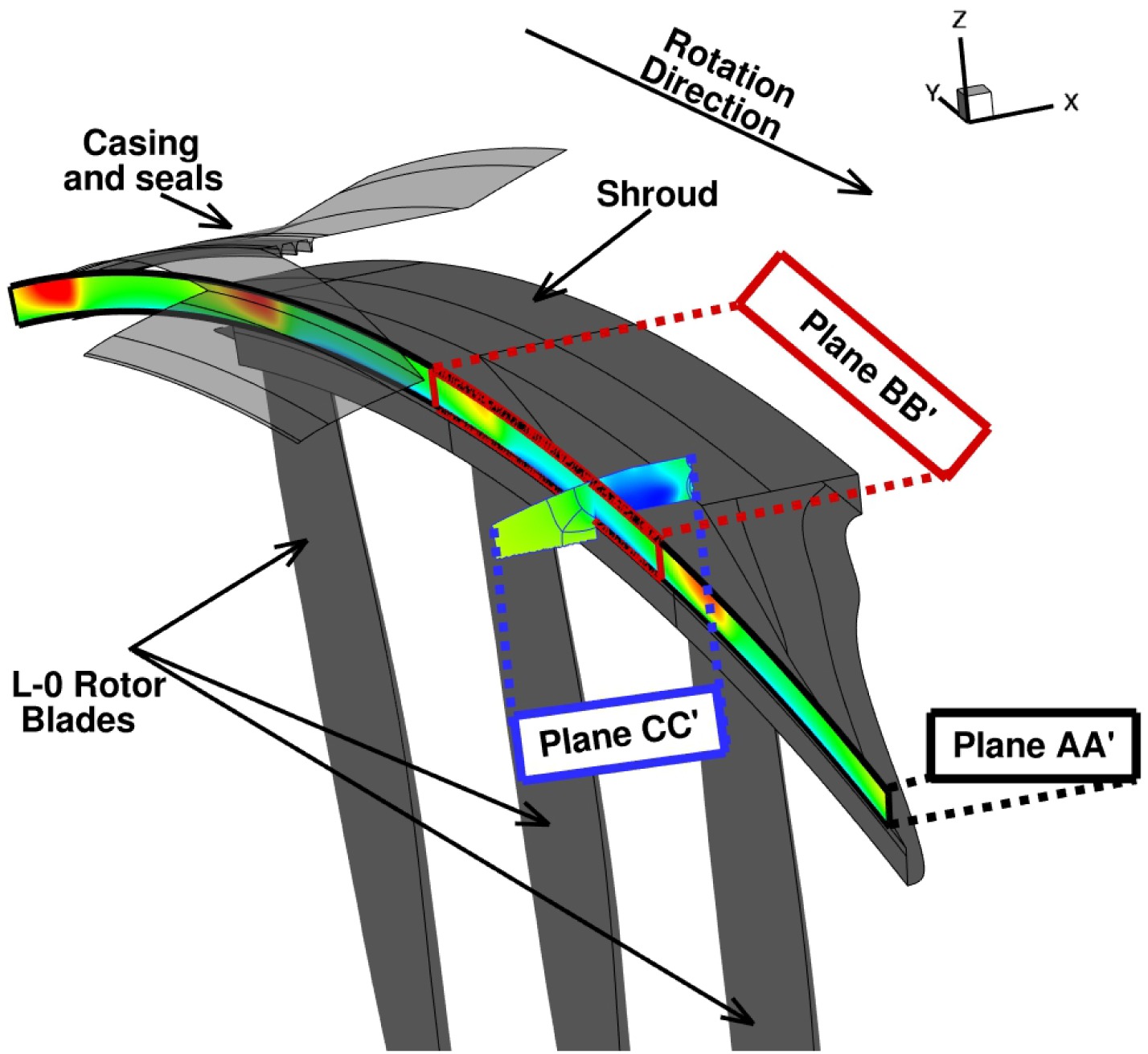
Figure 13 shows the planes for a specific time step, on which the analysis has been conducted. First, Plane AA’ was extracted along the full circumference of the sector (four rotor pitches). The plane is located exactly in the lip of the shroud. This location is selected because downstream there is an inlet separation bubble that is forming in the lip of the shroud and it would make it difficult to calculate accurately the mass flow without the amount being present inside the bubble. Additionally, plane BB’ equal to a single rotor pitch was extracted, in order to analyse the effect of the shock wave on the flow field and the mass flow. Finally, plane CC’ was extracted to gain insight of the flow field downstream of the inlet. All planes stay fixed in space and do not rotate with the rotor blades.
It was calculated that the mass flow through plane BB’ amounts to roughly ¼ of the total tip leakage mass flow on average through plane AA’ and shows peak-to-peak fluctuations of ±5.25%. These unsteady fluctuations are caused by the travelling shock wave, causing a mass flow redirection. The maximum amount was recorded on time step t/T = 0.233, while the minimum occurs on time step t/T = 0.787.
Figure 14 shows the flow quantities in plane BB’ for the two time steps that the minimum (right column) and maximum (left column) mass flow is monitored. Observer looks downstream in all figures and direction of rotation is from left to right.
Figure 14.
Plane BB’ — Circumferential distribution of Cps [-] (a-b), normalised axial velocity Cax [-] (c-d), and incidence angle [o] (e-f) at time steps of maximum (left) and minimum (right) mass flow.
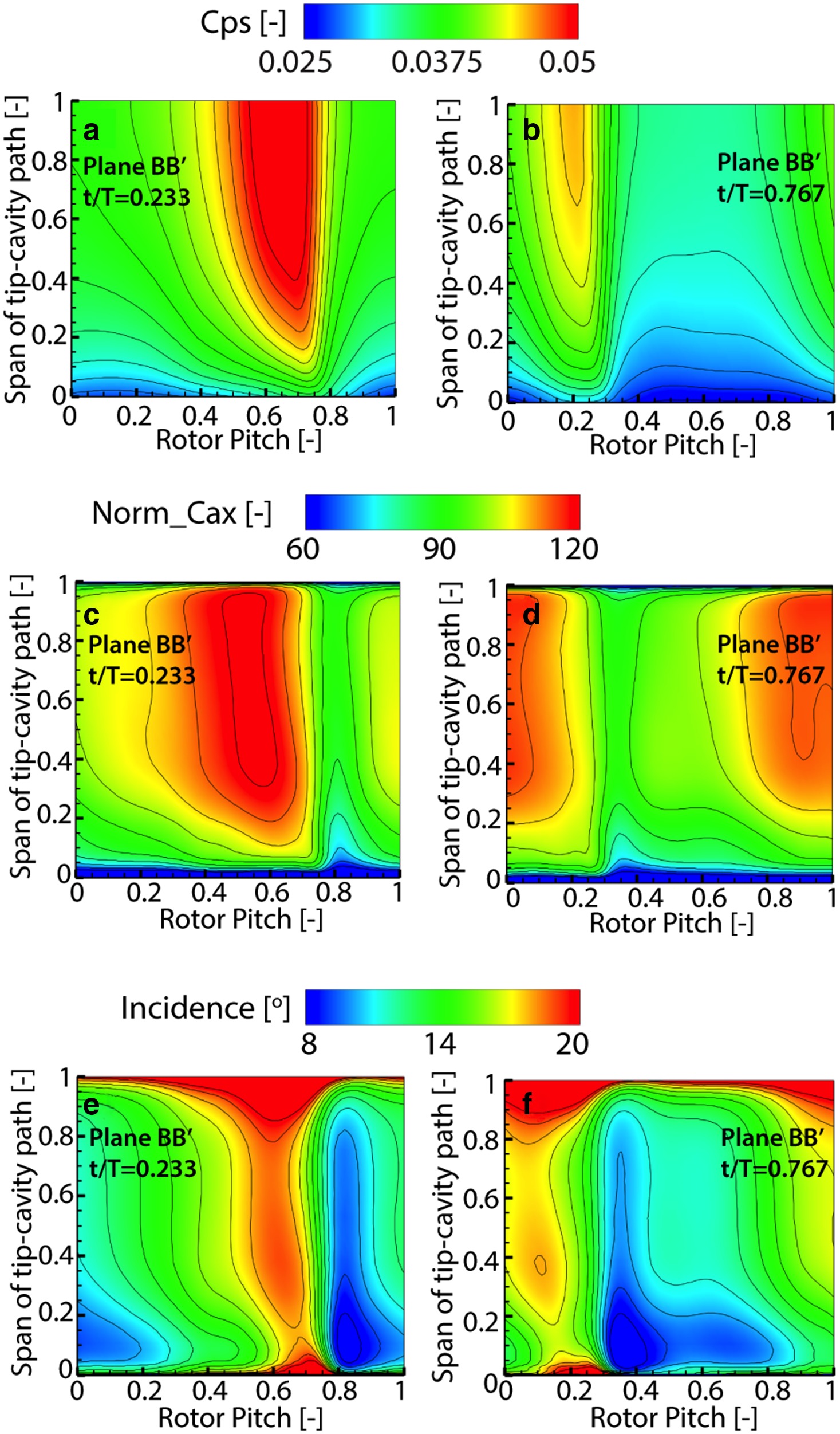
In Figure 14, there is a region of increased static pressure that presents a blockage in the flow, causing a redirection of the flow, as seen in Figure 14. Figure 14 shows the flow angle relative to the blade inlet angle of the rotor at 90% of blade span, essentially the incidence angle. Inside the region of increased static pressure, the relative Mach number decreases and the absolute Mach number increases. As the flow is redirected, the circumferential velocity decreases. Additionally, the downstream separation bubble, whose presence is desirable in that location to increase losses and reduce the leakage ingested in the cavity path, is suppressed in this time step as shown in Figure 15.
Figure 15.
Plane CC’ — Meridional view of Cps [-] at time steps of maximum (a) and minimum (b) mass flow.
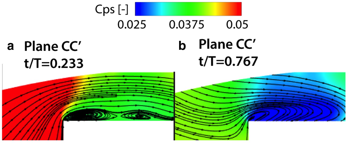
On the contrary, in Figure 14, it expands again causing additional blockage in the flow, as seen in plane CC’ in Figure 15. All these are leading to an axial acceleration of the flow in left time step and axial deceleration in the right time step, as presented in Figure 14 and Figure 14. Therefore, the mass flow shows its maximum value on the left time step.
It is interesting also to know the location of the shock wave relative to the upstream stator. This is presented in Figure 16, along with planes BB’ and CC’ as solid lines. It is observed that the maximum mass flow coincides with the time when the shock wave interacts with the suction side of the upstream stator when it reaches the trailing edge, while the minimum is recorded when it has overpassed it and high pressure region caused by the shock wave is located at throat of the upstream stator, looking in the third stator passage from the top.
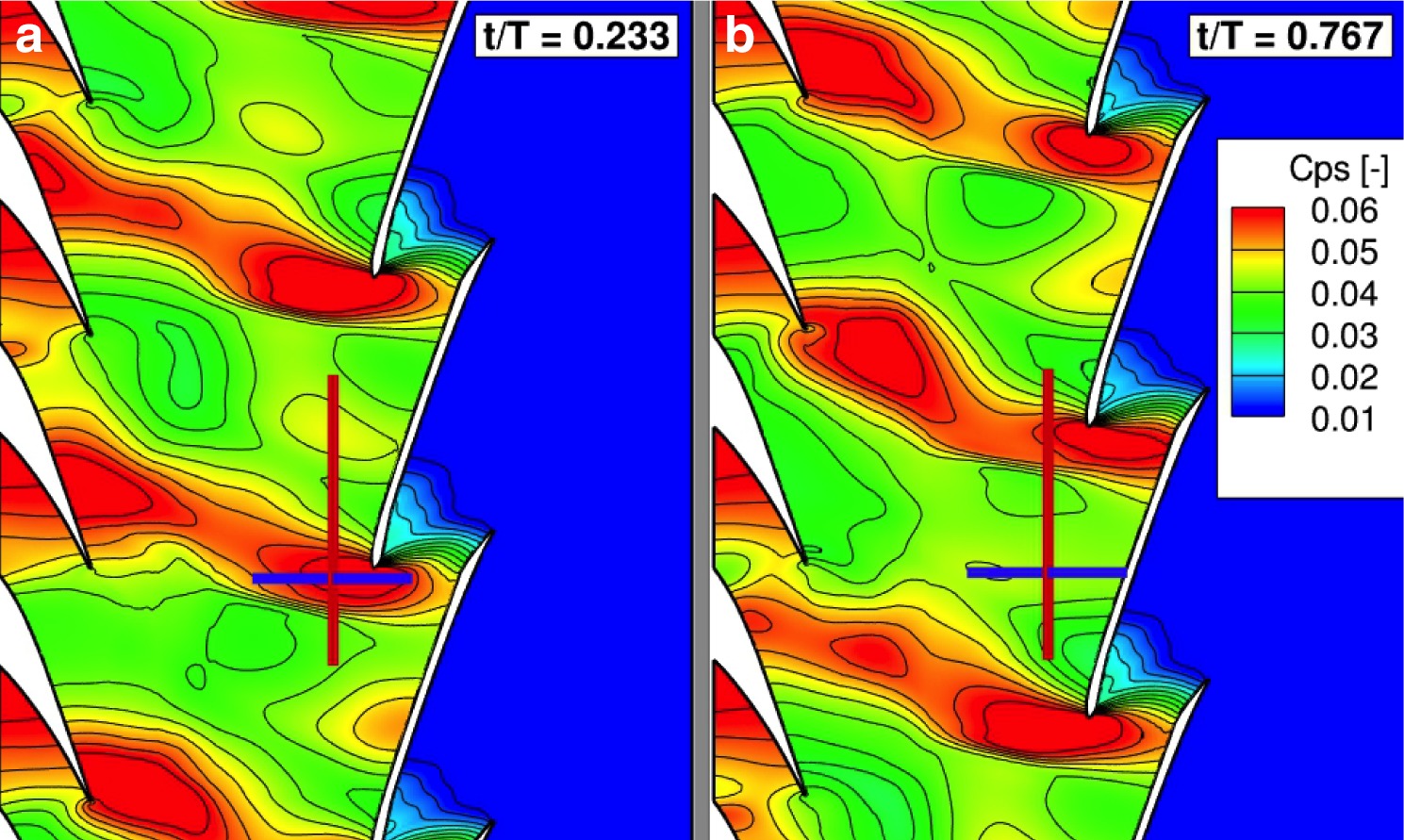
Despite the flow redirection and unsteadiness in time induced by the passing high pressure region, the total tip leakage mass flow that passes through the plane AA’ has been calculated to be 5% of the mass flow in the inlet of the L-0 stage and it is fairly steady with very low fluctuations at only ±0.2%. The area of this plane amounts to 1.98% of the whole available area at the specific axial location. These results need to be treated with caution though because the calculations occur in “cold state.” In reality, the high rotational speed along with the thermal load on the blade, definitely cause an expansion of the solid bodies, closing even further the available path and reducing the leakage flow.
Entropy generation in L-0 stage
To conclude the present study, entropy generation in the last stage of the low-pressure steam turbine is investigated. For this reason entropy loss coefficient is calculated for L-0 stator and L-0 rotor, separately. Definition of entropy loss coefficient is given in , where R is the individual gas constant for water vapour.
Figure 17 shows the time-averaged entropy levels in meridional view in the inlet of L-0 stator. Close to the casing, the entropy is high due to tip-leakage flow coming from L-1 rotor. The effect of this feature would be either lost or smeared out in case estimated boundary conditions were used in the absence of L-1 stage in the computational domain. This shows the importance of multistage simulations over single stage or single row simulations.
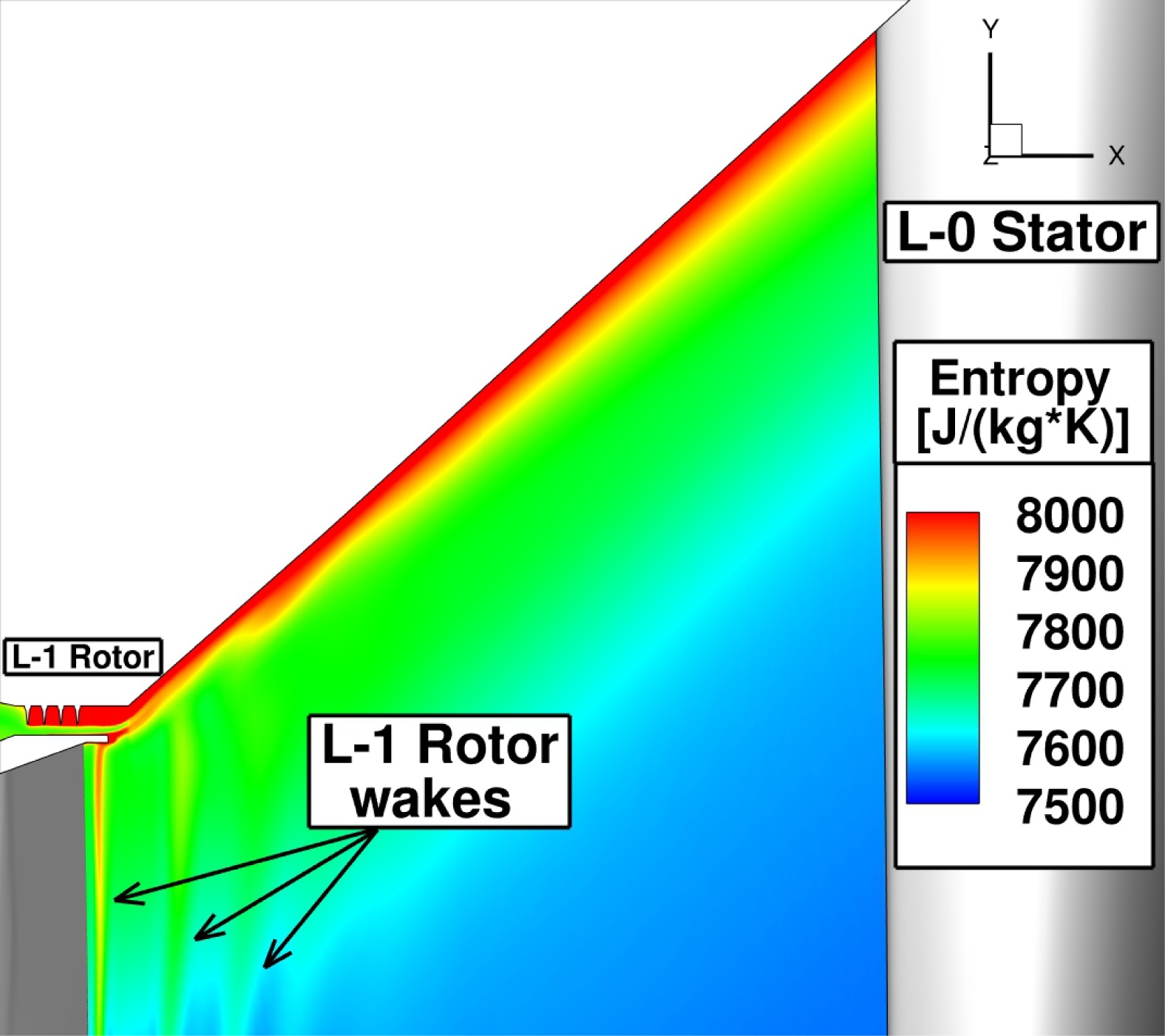
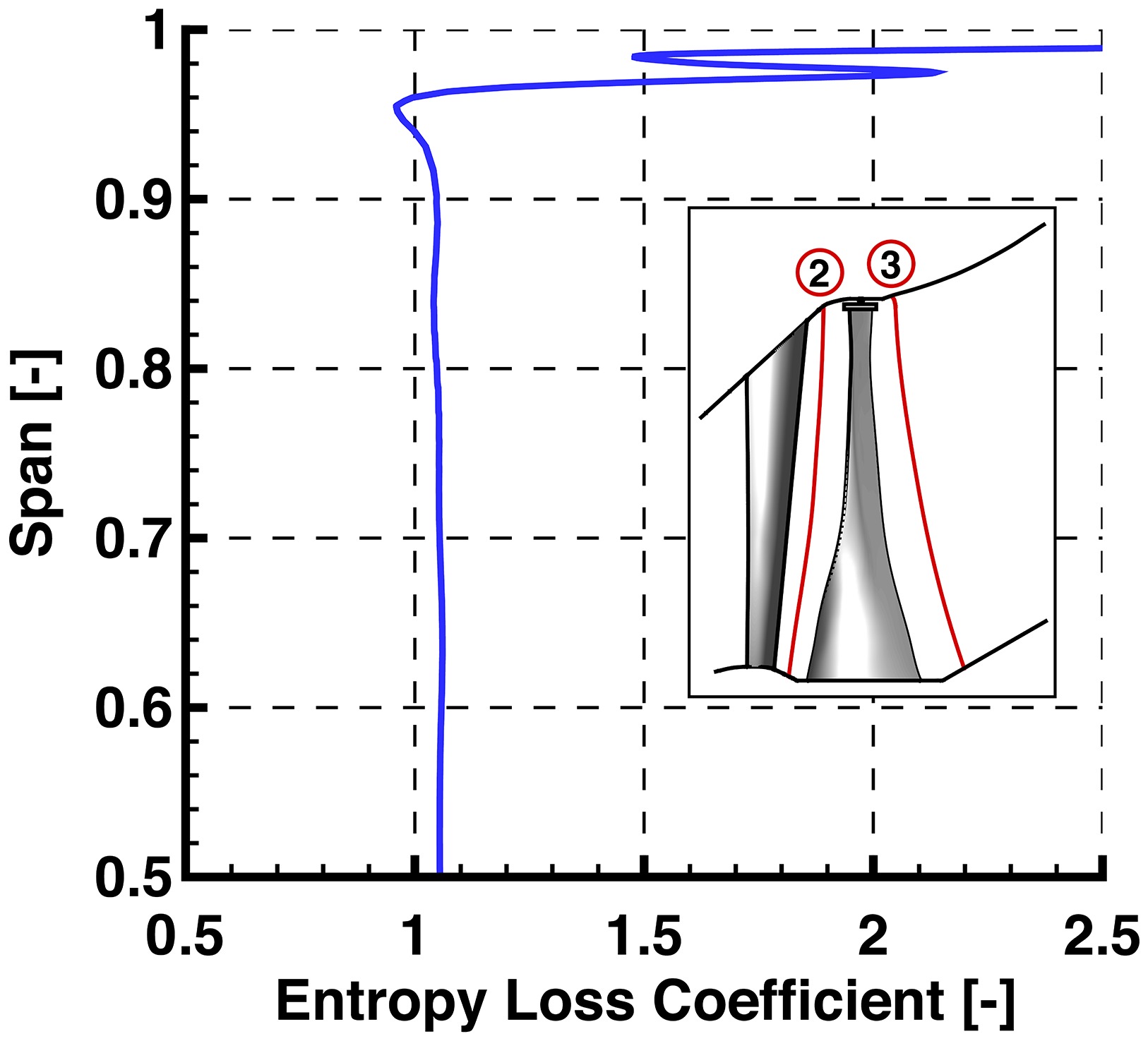
The entropy loss coefficient for stator is presented in Figure 18. Results are circumferentially averaged for one stator pitch and time-averaged for four rotor blade passing periods. Values greater and lower than one imply entropy increase and decrease relative to inlet in the according span position, respectively. Obviously, values are slightly greater than one due to entropy rise along the blade row.

The decrease observed in the last top 3% is due to radial migration of the tip-leakage flow coming from L-1, causing a local decrease of 23.4% at 99% span compare to mid-span. This loss transport is also contributing in the increase observed above 80% span, which is also induced by the travelling bow shock wave, causing a local maximum increase of 22.3% at 95% span compared to mid-span.
Similarly, Figure 19 presents entropy loss coefficient for L-0 rotor. Results are circumferentially averaged for one rotor pitch and time-averaged for four rotor blade passing periods. Slight decrease at 95% span also suggests radial transport of losses. The increase observed above 95% span is due to tip-leakage flow in L-0 cavity path. In that region, two peaks and a trough are present. The trough is in the middle of the leakage flow, while the peaks above and below it originate from the flow close to the solid boundaries of casing and blade span respectively. The local increase in the middle of the leakage flow, at 98% span, amounts to 42.3% higher compared to mid-span.
Apparently, the top 4% span of the full annulus is dominated by the effect of the tip-leakage flow, increasing entropy generation. However, it is important to mention again that the simulation was performed for “cold state” of the machine. In reality, the expansion due to rotational speed and thermal loads would close further the tip cavity path, limiting the entropy generation in a smaller percentage of the span.
Conclusions
The bow shock wave upstream of the leading of the last stage’s rotor causes locally an unsteadiness of ±34.4% in static pressure and ±10.4% in axial velocity, close to the suction side of the upstream stator, at 92.5% axial chord and 90% span.
Numerical results have been extensively validated with experimental data; time averaged 5HP and FRAP-HTH, as well as time resolved FRAP-HTH. In general, the numerical predictions with equilibrium steam modelling show good agreement with measurements, even under these extreme flow conditions. Flow quantities are predicted with RMS difference below 3.8o for yaw angle, 3.27% for relative Mach number, and 1.15% for total temperature.
The maximum fluctuation in time on suction side is greater than the maximum fluctuation in pressure side at the same axial location close to the trailing edge. This implies that there are moments in time where the blade is instantaneously counter-loaded locally in that location.
Despite the unsteadiness incurred by the periodic impingement of the shock wave on the suction side of the stator, there is no evidence of a boundary layer separation, even under these extreme flow conditions.
The maximum Cps recorded at 85% of stator axial chord is lower by 15.7% compared to 97.5% of stator axial chord. Additionally, there is a phase shift between the maximum values at these two locations equal to T/6 of the rotor blade passing period.
The mass flow passing through a domain equal to a rotor pitch in the inlet of the tip cavity of L-0 rotor shows an unsteadiness of ±5.25%, due to shock wave interaction and suppression of the inlet separation bubble in the lip of the blade shroud. Nevertheless, the flow is just redirected around the blockage and leads to a fairly steady inflow through the tip-cavity path.
The total tip leakage mass flow through the tip-cavity path was calculated to be 5% of the total mass flow, passing through 1.98% of the total available area in that axial location. However, results are derived for “cold state” of the machine, without taking into account the expansion occurred due to rotational speed and thermal load. Nevertheless, an estimation of ingested mass flow by the cavity path is crucial and can provide valuable information that needs to be taken into account from early steps of the turbine design.
Large stator-rotor gaps are crucial for the last stage of a steam turbine with long blades to allow the bow shock wave to weaken before it reaches the upstream stator. Additionally, the inlet separation bubble in the lip of the shroud would work more efficiently in the absence of stator-rotor interaction, reducing the ingested leakage flow. Forward sweep of the stator blade close to the tip is a potential solution in cases where limitations in bearing location do not allow increase of axial distance between stator and rotor of the last stage.
Calculation of entropy loss coefficient for stator and rotor in the last stage reveals the effect of bow shock wave and tip-leakage flow on entropy generation, respectively. Regarding the stator, a decrease of 23.4% compared to mid-span is observed at 99% span due to radial migration of leakage flow coming from L-1 stage to lower span position. This loss transport, along with the effect of the bow shock wave, contributes to a local maximum increase of 22.3% compared to mid-span, at 95% span. Finally, the inevitable entropy generation due to tip-leakage flow in L-0 rotor amounts to 42.3% at 98% span and its presence affect the top 4% of the full annulus. However, results are derived in “cold state” of the machine, so an over-prediction of the effect compared to reality is expected.
Results presented in the current work highlight the importance of performing multistage simulations, as well as unsteady simulations, instead of steady state.
Nomenclature
Cps
Static Pressure Coefficient
[-]
P
Pressure
[Pa]
T
Temperature, Time period
[oC]
Ma
Mach number
[-]
Cax
Normalized Axial velocity
[%]
q
Entropy Loss Coefficient
[-]
S
Entropy
[J/(kg*K)]
R
Individual Gas Constant for water vapour = 461.5
[J/(kg*K)]
Abbreviations
MHPS
Mitsubishi Hitachi Power Systems, Ltd.
LP
Low pressure
GP-GPU
General Purpose - Graphic Processing Unit
CSCS
Swiss National Supercomputing Centre
LEC
Laboratory for Energy Conversion
CFD
Computational Fluid Dynamics
URANS
Unsteady Reynolds Averaged Navier-Stokes
MPI
Message Passing Interface
5HP
5-hole probe
FRAP-HTH
High temperature, fast response aerodynamic heated probe
PSC
Part-span connector
RMS
Root Mean Square
PS
Pressure side
SS
Suction side
TE
L-0 stator trailing edge
Fq
Flow field quantity (pressure, yaw, etc.)