Introduction
Combustion systems of conventional stationary gas turbines are designed to achieve low emissions at high load operation. For gaseous fuels typically swirl-stabilized premix burners are used. With the increasing amount of renewable power in recent years high load flexibility of gas turbine power plants has gained in importance. Traditional combustors suffer from strongly increasing emissions with decreasing load. Presently, low emissions of CO (10 ppmv at 15% O2) can be achieved down to about 40% load. To increase its competitiveness, industry is targeting low emissions down to 20% load. In order to achieve a wide load range at low emissions an axially staged lean-lean combustion system is proposed here. Apart from a wide load range and earlier have both demonstrated that lean-lean staging also has the potential for low nitrogen oxides (NOx) at full load. Due to the sequential arrangement of the stages in an axial manner, NOx emissions can be kept low by limiting the residence time at high temperatures.
Figure 1 shows the basic concept. The stage 1 premixing combustion chamber is fed with roughly half of the compressor air and is always in operation. The second half of the compressor air is fed to the stage 2 chamber, where it mixes with the hot products of stage 1. At low load there is no fuel fed to stage 2 and hence no flame in the stage 2 chamber. Above a certain load stage 2 air is supplied with fuel and the mixture is ignited by the hot stage 1 products. Whereas on the test rig the air split “stage 1/stage 2” can be varied (optimization parameter), that split would be fixed on a real gas turbine.
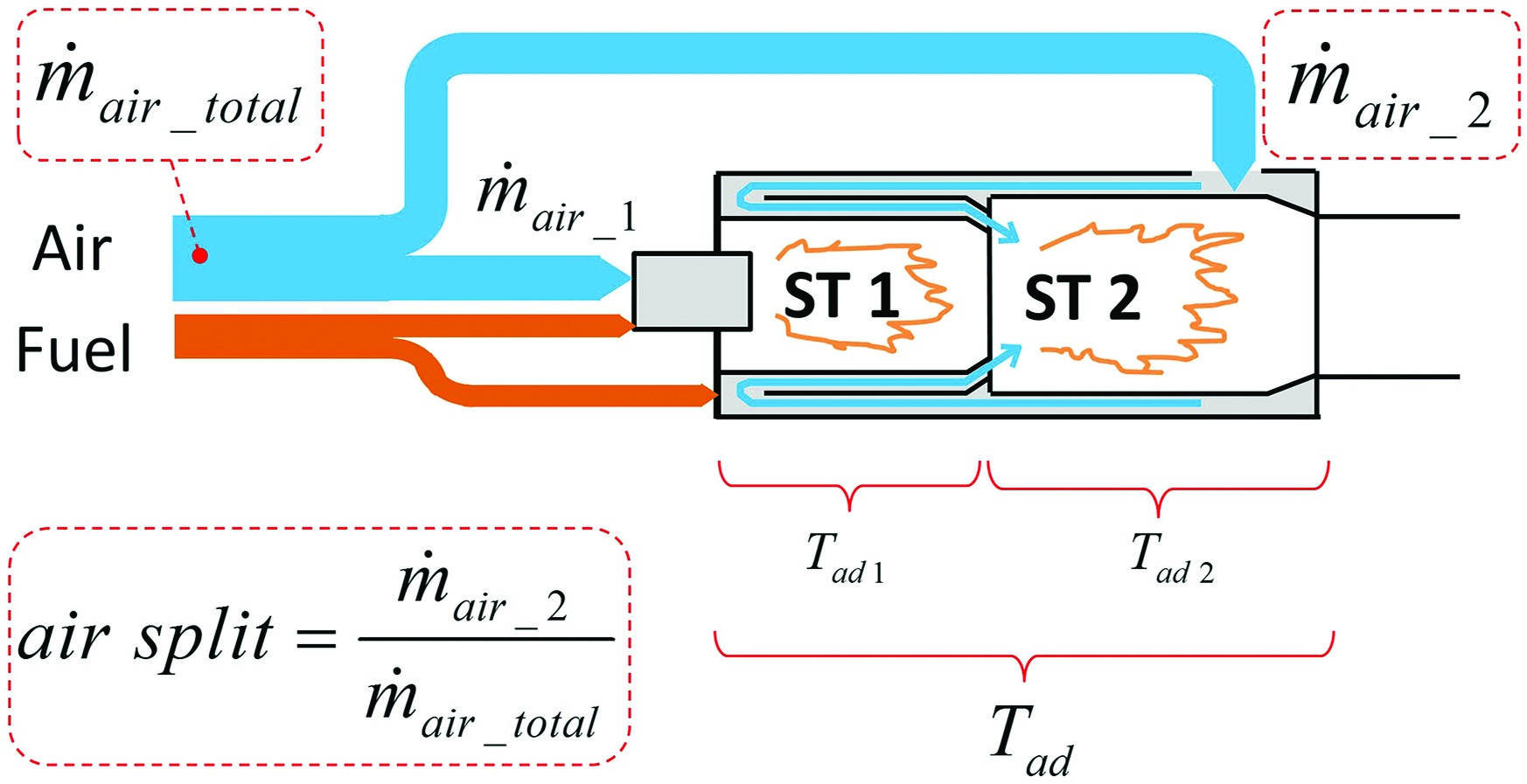
The present paper focuses on the development of the mixing section between first stage hot gases and the second stage fresh mixture.
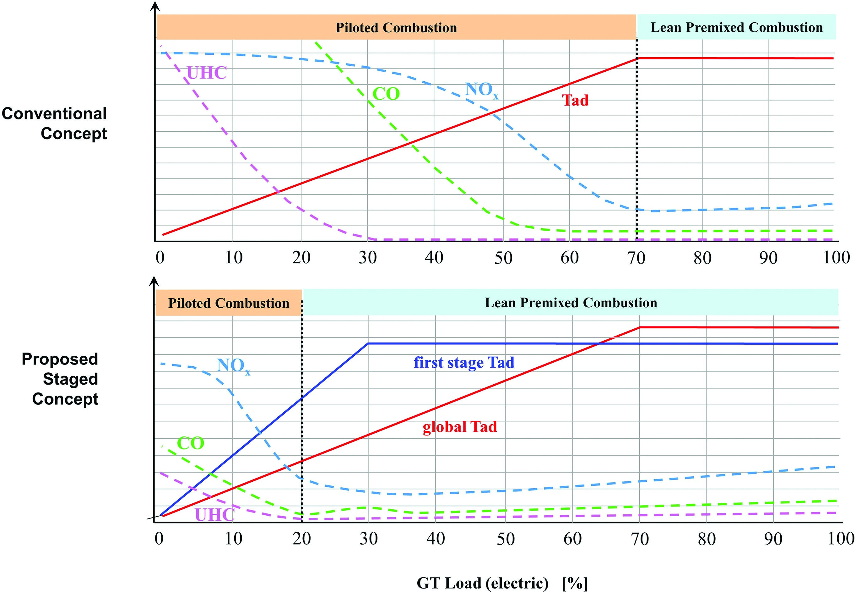
The upper diagram in Figure 2 shows the typical situation of increasing emissions towards lower load, which is usually due to the not premixed piloted system coming into operation when proceeding from full load to part load. The lower diagram shows the targeted characteristics that shall be achieved with the staging concept as described here.
Methodology
Several steps are needed for the development of a combustion system, starting from 1D calculations, kinetics simulations, CFD cold and hot simulations, atmospheric and full pressure combustion tests up to the final engine tests. In the present study high pressure combustion tests have not yet been carried out. However, the authors are confident that the trends seen in the atmospheric combustion are well suited to allow predictions of the characteristics under full engine pressure.
Experimental setup, investigated configurations
Figure 3 shows the setup of the atmospheric test combustor. The two chambers have separated supplies of preheated air and fuel gas. Three configurations of the mixing section have been tested. Adiabatic flame temperatures for each stage and in average have been determined from measured mass flows and inlet temperatures. The cylindric walls of stage 2 chamber were made of quartz glass, allowing flame pictures in the visible and UV range.
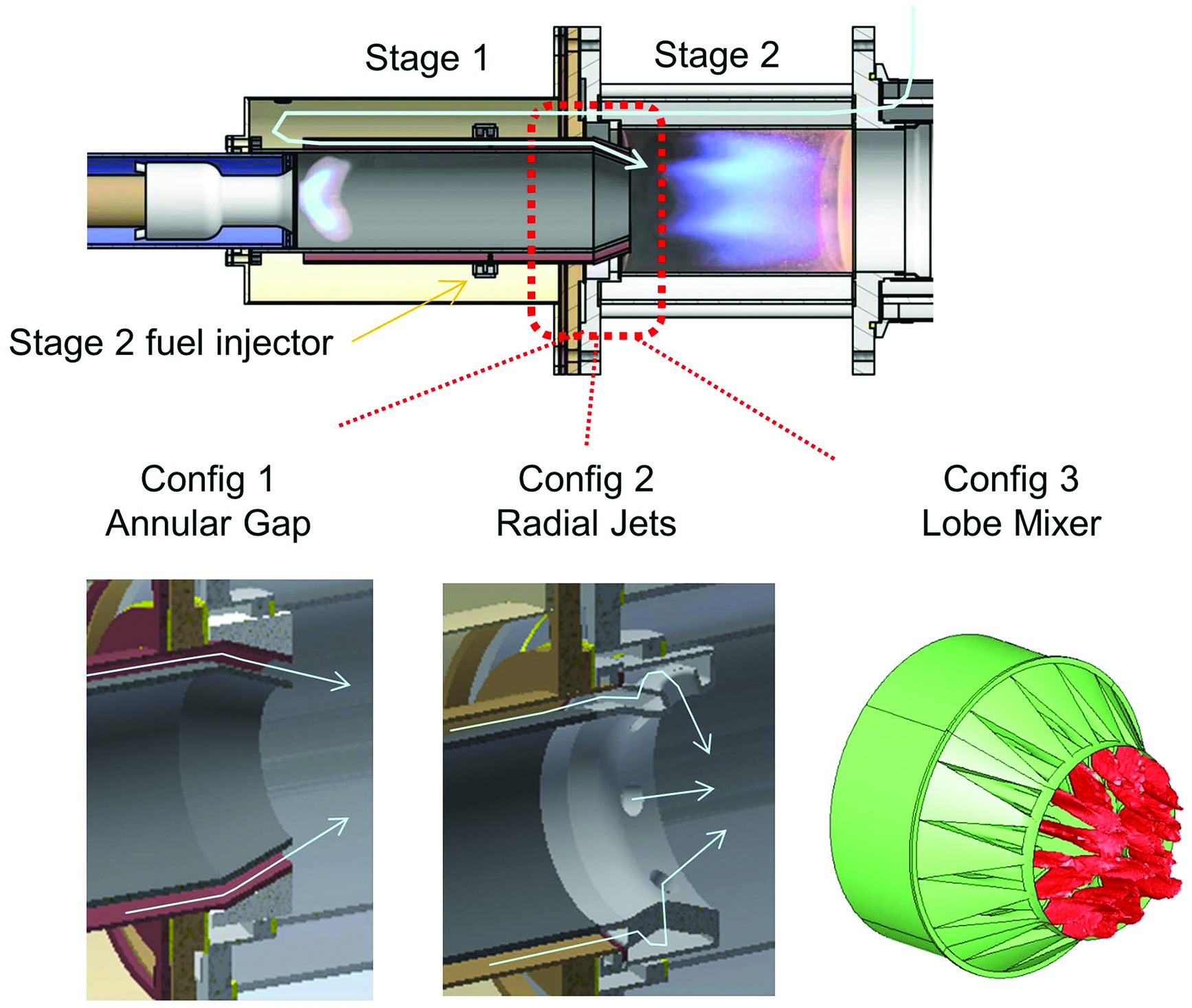
The motivation for the selection of the three mixing configurations was:
Config 1 Annular gap: This simple geometry serves as baseline.
Config 2 Radial jets: Basically a higher mixing quality can be achieved. The number of holes and the hole diameters were determined by 1D correlations 04.
Config 3 Lobe mixer: An again better mixing quality as compared to radial jets was expected.
For configurations, 2 and 3 the details of the geometry were determined based on CFD results, see chapter below.
Test results
Subsequent diagrams show the results of the combustion tests. If not stated differently, the setup was as follows:
Combustor pressure: atmospheric.
Fuel: natural gas (6% [vol.] C2+).
Air inlet temperature to both stages: 450°C.
Burner 1 position/chamber length constant.
Emission values: normalized to 15% O2, O2 measured at exit of stage 2 combustor.
Relative pressure drops over the total combustor were always <5%.
Figure 4 shows pictures of stage 2 flames for the three mixing configurations at three different flame temperatures. Whereas pictures on the left side show visible light, on the right side pictures of a UV sensitive camera with a narrow filter in the UV range are shown, representing the OH concentration and hence the intensities of the chemical reaction. The flame with Config 1 seems to be well anchored and rather compact but not symmetric. The Config 2 flames appear more compact as compared to the Config 1 flame but are more distributed. Config 3 obviously shows completely different flames as compared to Config 1 and Config 2. The reaction zone is long and it looks rather detached from the mixing section. More explanations will be given in the CFD section below.
Figure 4.
Left side: flame photos in visible range, right side: OH Chemiluminescence. All pictures for air split 50%, at adiabatic flame temperatures as indicated on top.
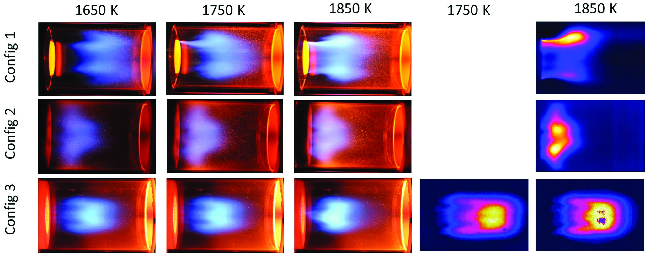
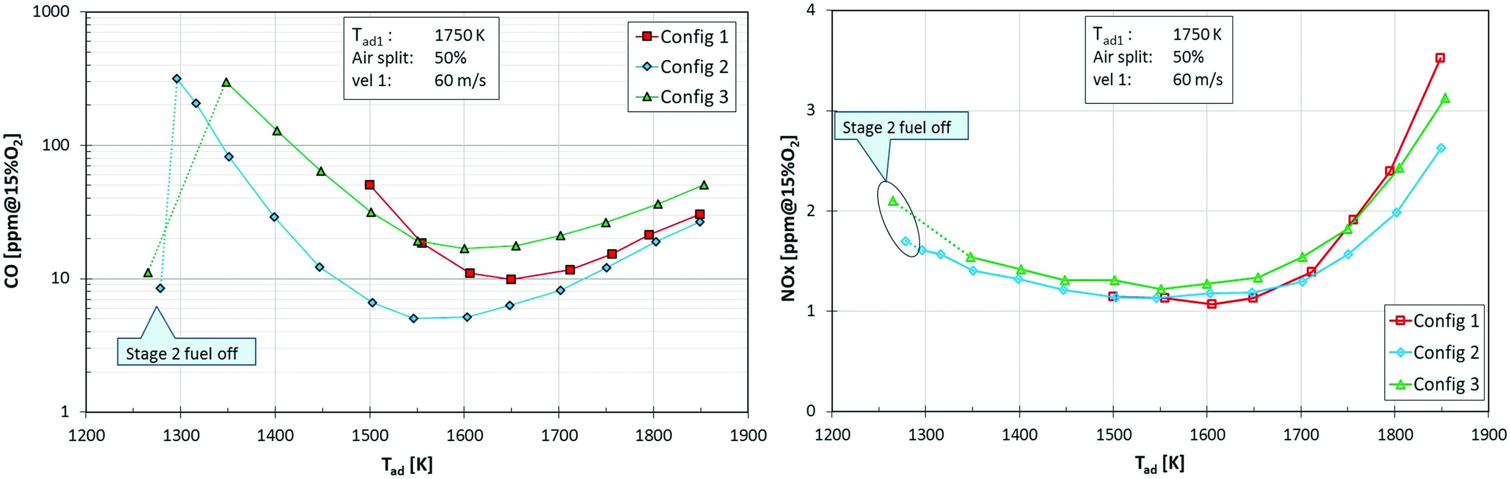
Figure 5 shows NOx and CO emissions for all configurations. The three configurations do not show significant differences in the NOx emissions. The fact that the NOx vs flame temperature curve shows a minimum might look unusual on first look. The absolute amount of produced NOx increases continuously with the flame temperature; the mentioned minimum stems from normalization to 15% O2. For stage 2 switched off, the stage 1 combustor, if run at 1,750 K, emits about 2 ppm NOx. Interestingly, the same normalized NOx value is observed if both stages are in operation with an average temperature of 1,750 K. This means that in both stages the NOx production per mass of fuel is about the same. Production of thermal NOx is expected to be low on this test rig due to low pressure (atmospheric), relatively high heat loss and hence fast reduced hot gas temperatures (at high combustor pressures thermal NOx and residence times will be important). The CO curves in Figure 5 show minima in the range 1,500 K to 1,700 K. The increase towards higher flame temperatures can be explained with equilibrium CO, whereas the increase towards lower flame temperatures is due to local quenching effects. When switching off the stage 2 fuel, CO emissions drop by an order of magnitude. This behavior was expected. Proper CO burnout requires a minimal flame temperature. In terms of width of the operable flame temperature range Config 2 is the best. The increase of CO happens at roughly 100 K lower flame temperatures as compared to Config 1 and 3.
Figure 5.
Emission of Config 1, 2, and 3 as a function of the flame temperature. Left side: NOx, right side: CO.
The left side diagram in Figure 6 shows the influence of flame temperature variation in stage 1. NOx is increased, if stage 1 is run at higher flame temperatures. Interestingly, as long as both stages are in operation, CO emissions at a given overall Tad are roughly independent of stage 1 flame temperature. When switching on stage 2, high CO values are observed until stage 2 fuel massflow reaches a level at which a stable flame can exist. The higher the stage 1 temperature, the lower this CO peak. The increase of CO towards higher overall Tad can be explained by an increase of CO equilibrium concentration. This increase will not be as significant at high pressure conditions which will be found in the engine.
Figure 6.
Emission values for Config 2. Left side: CO and NOx emission as a function of the overall flame temperature, for different flame temperatures in stage 1. Right side: CO and NOx emissions as a function of the thermal power (second stage switched off at low load).
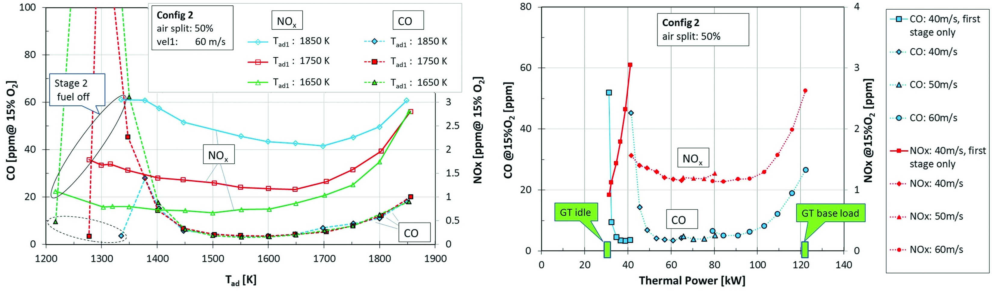
Gas turbines are usually equipped with variable inlet guide vanes at the compressor inlet, which allows variation of the air mass flow over load. The right side diagram in Figure 6 shows a test where the thermal load was varied both by incremental steps in burner velocity and by increasing the flame temperature (on a real gas turbine air mass flow increases without significant change of the burner velocity, since the combustor pressue increases as well). An increase of the thermal load from about 20% to 100% corresponds to an output power variation of a gas turbine from idle to full load. The results show that the staged system provides a wide load range at acceptable emissions.
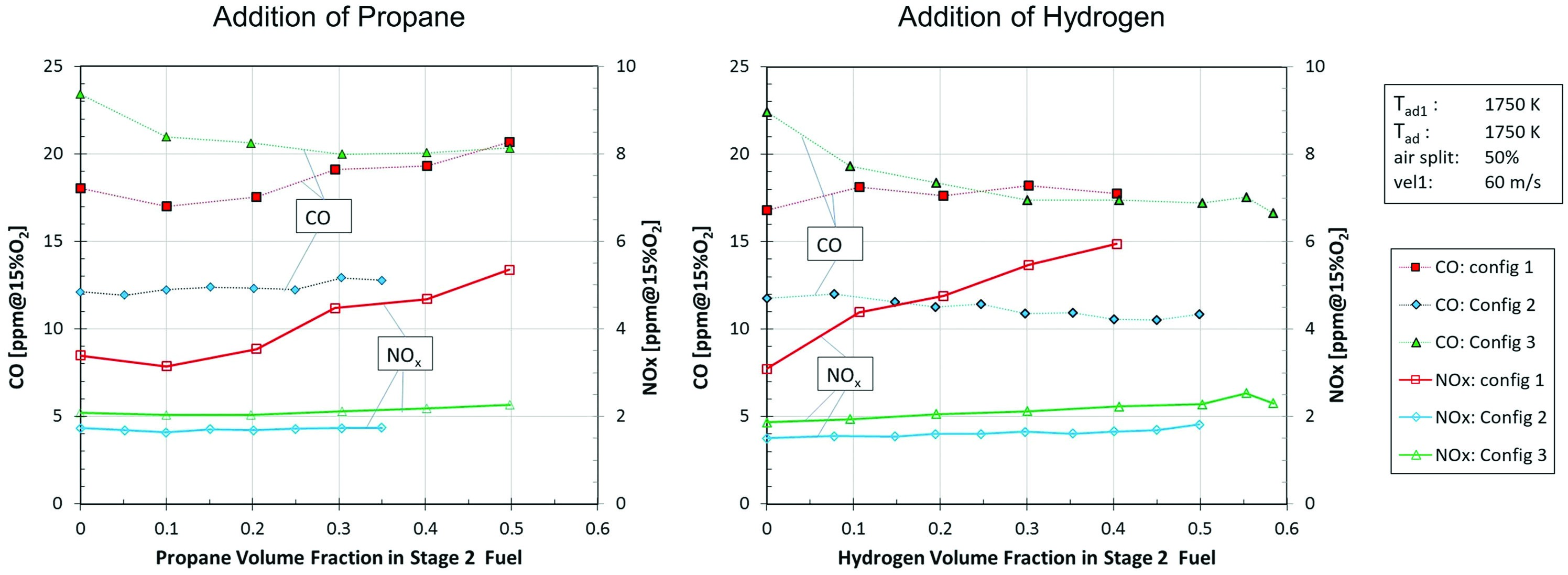
Figure 7 shows the behavior of the staged combustion system when blending the stage 2 fuel with propane or hydrogen, which increases the reactivity of the fuel. On the one hand this gives an idea about the robustness of the system against variation of the fuel composition as can happen in natural gas systems. On the other hand an increase of the reactivity is expected to show similar changes of the flame characteristics as caused by an increase in combustor pressure. The trends as seen by adding propane are very similar to adding hydrogen. Config 1 (annular mixer) shows the strongest impact on emissions. With increasing amount of propane or hydrogen CO and NOx emissions go slightly up. This can be explained by an enrichment of the reaction zone since there is less time for mixing due to the increased reactivity of the fuel. Config 2 (radial jets) shows almost no variation of the emission with variation of the fuel. The mixing quality apparently is hardly influenced by the increased reactivity of the fuel. Config 3 shows a reduction of CO when adding propane or hydrogen. A likely explanation is that due to the increased reactivity the flame establishes itself further upstream and becomes more compact. As a consequence there is more chamber length available for CO burnout. Regarding NOx the opposite trend applies. The mixing distance until reaching the reaction zone is slightly reduced leading to slightly higher NOx. What happens to the Config 3 flame when adding more reactive fuel is what is also expected when operating at high combustor pressure. Whereas in terms of fuel robustness Config 2 seems to be the best in the atmospheric tests, it might well be that under full engine pressure Config 3 would turn out to be the best variant.
Numerical simulation, comparision with experiments
The ignition source for the stage 2 mixture is primarily the hot exhaust gases from the stage 1 flame. Once ignited the flame would propagate through the stage 2 mixture at a rate governed by the turbulent burning velocity. One way to speed up the combustion process in order to minimize the flame length required to fully oxidize CO is to increase the rate of mixing between stage 1 and stage 2. Minimising the flame length has the added advantage that the combustor length can be reduced reducing residence time and hence NOx emissions.
Thus to optimize this design CFD was used initially to optimize the mixing process between the first and second stages. Later, when CO emission measurements were not found to correlate with predicted mixing trends, further analysis was performed to try to understand this discrepancy.
Numerical setup
The commercial CFD code ANSYS CFX was used to solve the steady-state Reynolds averaged Navier Stokes equations. Reynolds stresses were closed using the Shear Stress Transport turbulence model. Heat release was modelled using the standard Eddy Dissipation combustion model 01. This model assumes that chemistry is infinitely fast compared to mixing and thus the heat release rate is limited only by the mixing rate between hot products and fresh mixture.
To simplify the problem the first stage with the premixed flame was not included in the domain. Its velocity, turbulence and temperature profiles were patched at the exit of stage 1 from a separate detailed simulation of this stage. A fully premixed fresh gas was introduced at the inlet of stage 2. On the atmospheric test rig the fuel air mixing of stage 2 was not perfect. Fuel was injected through discrete jets on the outer wall of the stage 2 supply annulus. Thus, as the flame temperature increased, the penetration of the fuel jets would also increase placing more fuel radially closer to the axis of the burner. This was expected to impact Config 1 and Config 3 more than Config 2. Config 2 had a more tortuous flow path between the fuel injection and the stage 2 injection nozzles allowing for greater premixing of the fuel and air. However it is believed from the analysis and comparison with the measurements that the impact of the real fuel distribution is secondary to the main effects identified.
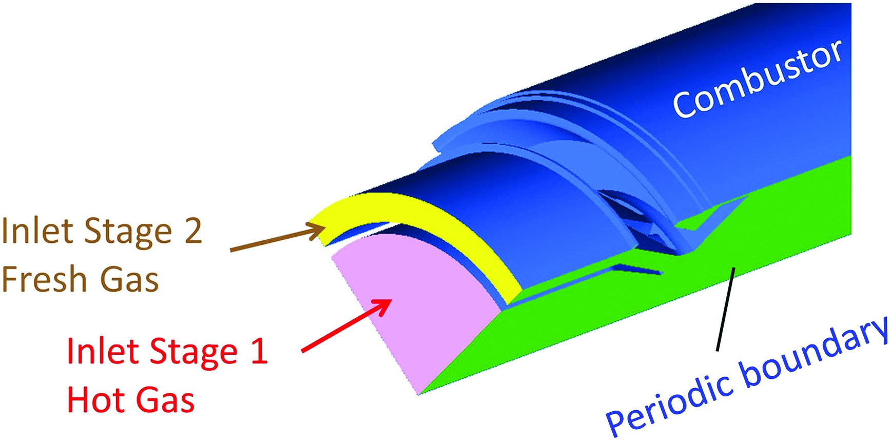
A periodic quarter of the test rig was simulated to reduce computational effort, see Figure 8. To capture the mixing characteristics of the two stages more accurately, the grid in the mixing zone was further refined.
For the CFD study operation conditions from the test rig were used. A flame temperature of 1,750 K was adopted for both stages and an air flow split of 50:50 between the stages was set. Finally all of the walls were assumed to be adiabatic.
Mixing of the second stage
In order to assess the mixing a conserved scalar was introduced at the inlet to stage 2 with a value of 1. This scalar represented the mixture fraction of stage 2 gases and acted as a tracer of this flow.
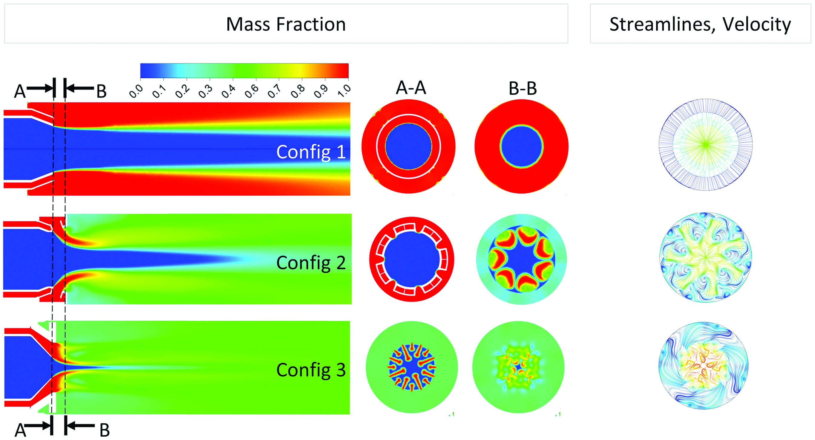
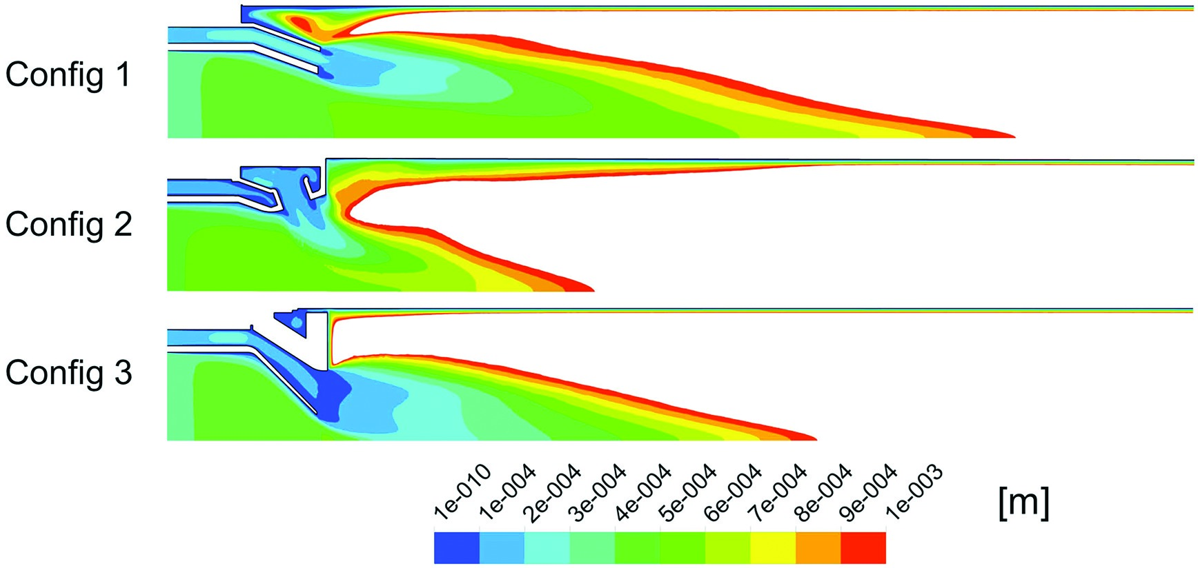
Contour plots of this scalar can be seen for each of the three configurations in Figure 9. Plane A-A is located at the exit of the nozzle and plane B-B is located 2 cm further downstream.
Figure 9.
Mass fraction of stage 2. In-plane streamlines in B-B plane coloured by velocity magnitude (m/s).
To further quantify the mixing a spatial unmixedness parameter, U, was derived from the work of . This was calculated at cross sections perpendicular to the burner axis with the following formulation:
where Z is the mixture fraction of the stage 2 gas and the over bar indicates a mass flow weighted averaging over each cross section considered. Figure 10 shows how the unmixedness parameter varies along the burner axis. Config 3 followed by Config 2 are predicted to have the best mixing.
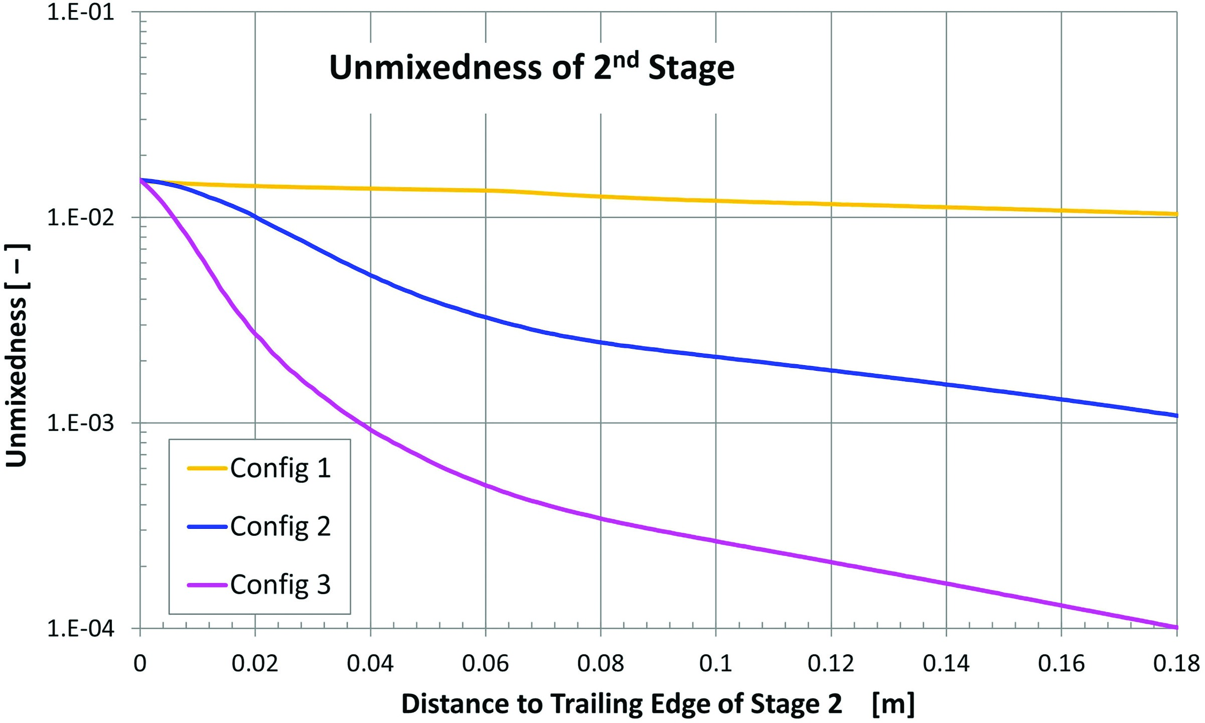
Config 1 which consists of a complete annulus around the stage 1 nozzle mixes only along the shear layer between the two flows. Both Config 2 and 3 increase the size of this shear layer either by introducing discrete jets in the case of Config 2 or by highly corregating the shape of the stage 2 injection nozzle in the case of Config 3 (Figure 3). This increased surface area is responsible for an initial burst in the mixing rate over a relatively short distance.
Both Config 2 and 3 also drive large scale secondary motion through the interaction of the flow from stage 2 with the flow from stage 1 further enhancing the mixing over longer distances. The jets of Config 2 roll up forming horseshoe vorticies which will further entrain hot stage 1 gases and enhance radial and circumferential mixing. The nodes of Config 3 are designed to impart a radial inward component to the stage 2 momentum which will produce large scale vorticies when this flow mixes with the stage 1 gases. The large scale secondary flow produced by both Config 2 and 3 is visible in a plot of in-plane streamlines at the B-B plane, see right side pictures in Figure 9. These pictures also highlights through the velocity magnitude that the contraction of both the stage 1 and 2 nozzles at the mixing plane for Config 3 are significantly greater than for either Config 1 or Config 2. Table 1 quantifies this greater contraction which was introduced to further harden the combustor against potential thermoacoustic problems which might occur in a commercial gas turbine version of the combustor. However this will also cause the axial momentum to be increased and hence residence time of the bulk flow in the core of the combustor to be significantly reduced, which may be a large factor contributing to the higher CO emissions for this configuration.
Flame analysis of the second stage
Despite a significant increase in predicted mixing performance atmospheric measurements of Config 3 indicate that it has the highest CO measurments (Figure 5). This contradicts expectations that improved mixing will reduce the flame length required to fully oxidise CO.
As was already mentioned this may be partly due to the higher axial momentum and reduced residence time in the combustor for this configuration, which will have the effect of stretching the flame axially. Figure 4 seems to confirm this as the flame length is stretched significantly downstream.
To explore this further contours of turbulent flame speed Ut were post processed on the predictions made with the Eddy Dissipation model. For Ut a correlation provided by was used, which partially considers finite chemistry effects:
where A is the model constant of 0.52, u’ the turbulent velocity, Ul the laminar flame speed, which was assumed to be 0.7 m/s, α the unburnt thermal diffusivity and lt the turbulence length scale.
Figure 11 illustrates contours of this flame speed plotted for each of the three configurations. On these contours an iso-line of the stage 2 mixture fraction equal to 0.6 is plotted. Provided the assumption of infinitely fast chemistry holds true and there is no flame quenching, this line gives an indication of the ignition front of the stage 2 gases.
Figure 11.
Turbulent flame speed [m/s]. The black line indicates the iso-line of stage 2 mixture fraction Z = 0.6.
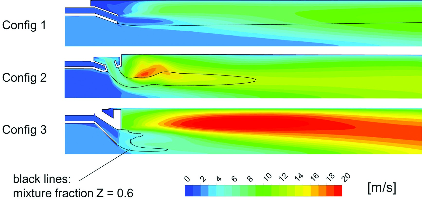
It is interesting to note that the iso-line of stage 2 mixture fraction appears to confirm that the improved mixing of Config 3 should bring the ignition of a greater fraction of the flame closer to the exit of the stage 1 exit. However the predicted turbulent flame speed immediately downstream of this ignition front is much lower for Config 3 than Config 2 and as such for the same axial velocity one would expect that the flame propagation would require a greater axial distance.
Looking at the ratio of the axial component of the velocity normalized by this turbulent flame speed (Figure 12) one can clearly see that this effect is made significantly worse by the higher axial velocity component of Config 3. This fits very well with the measurements of flame length pictured in Figure 4.

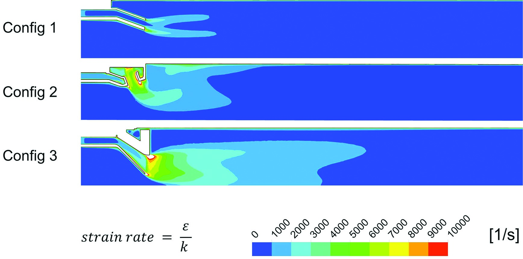
Contours of turbulence length scale (Figure 13) explain why the turbulent flame speed is predicted to be so low in the wake of the stage 1 exit for Config 3. The corregated lobes of Config 3 which increase the surface area between the stage 1 and stage 2 gases generate a lot of small length scale turbulence in the shear layer between these two flows. This turbulence dissipates very quickly as can be seen in contour plots of the ratio of the turbulence dissipation rate to the turbulence kinetic energy otherwise known as the turbulent strain rate (Figure 14). For Config 3 there is a large zone of large length scale turbulence which is generated in the shear layer between the high speed jet in the core of the combustor and the outer recirculation zone. This produces the region with high predicted turbulent flame speed at the outside edge of this nozzle flow. Unfortunately this region does not contribute significantly to the combustion of the stage 2 gases in the core of the combustor which is where the flame is predicted and measured to occur (Figure 4).
The jets in Config 2 are predicted to generate more significant quantities of large scale turbulence (Figure 13) which takes longer to dissipate, hence turbulence levels persist longer and the turbulent flame speed is predicted to be higher. This in combination with the lower axial momentum of the flow leads to a much shorter length required for flame ignition and propagation when compared to Config 3.
Additionally while high levels of turbulence generally leads to higher burning rates excessive levels of turbulence can lead to flame quenching due to high diffusion rates of heat and radicals away from the flame front. Turbulent strain rate (Figure 14) is generally considered an indicator of the potential for flame quenching. Both Config 2 and Config 3 have very high strain rates in the vicinity of the stage 2 nozzle exit. This level drops off faster for Config 2 and does not persist as far downstream. Therefore the potential for flame front quenching producing a lifted flame is higher for Config 3. The OH chemiluminescence images in Figure 4 appear to suggest that the flame is actually lifted off of the stage 1 exit and starts further downstream than for Config 2. Care needs to be taken when drawing this conclusion because it depends on the contrast of the images and it may be that very low OH luminosity is present close to the burner. However the predicted high strain rates do suggest that flame lift off is a real possibility.
Thus the rapid dissipation of the shear layer turbulence generated by the wake of the lobe mixer in Config 3 combined with the reduced amount of large scale turbulence compared to Config 2 leads to lower turbulent burning velocities and reduced flame propagation rates for Config 3 compared to Config 2. This combined with the significantly higher axial momentum of the flow leads to an axial stretch of the flame and higher CO emmisions. On top of this the high dissipation rate at the nozzle exit leads to high turbulent strain rates which has the potential to quench the flame lifting it off of the stage 1 nozzle exit pushing the flame further downstream and making the CO emissions even worse.
Conclusions
Atmospheric tests and CFD investigation of the proposed lean-lean staged combustor concept have demonstrated the potential of the concept for application in a stationary gas turbine. The staging concept allows low emission operation over a considerably wider load range as compared to conventional gas turbines. Specific results are:
The load can be reduced from 100% to about 20% while maintaining acceptably low CO and NOx emissions.
No diffusion-type piloting is required for flame stability.
The configurations of mixing sections between stage 1 and stage 2 were designed such that overall combustor pressure drops always stayed below 5% (relative).
The design of the mixing section between stage 1 and stage 2 is crucial. Fresh stage 2 gases should mix very efficiently with the hot stage 1 gases. However, apart from the mixing quality also proper flame anchoring needs to be provided. The configuration with the best unmixedness parameter was found to be unsatisfactory regarding CO emissions, since the reaction was found to occur too far downstream, leading to insufficient residence time. The stage 2 design, in which gases are introduced by radial jets, was found to be the best configuration; however, this was carried out with a low stage 1 hot gas velocity and it is thus not possible to unequivocally state this will always be the best design for all ranges of stage 1 velocity.
For design optimization based on CFD simulation, the following criteria are proposed: first the unmixedness (stage 2/stage 1) in the flow direction shall drop as quickly as possible. Second, downstream of the predicted ignition front, the turbulent flame speed shall be sufficiently high without excessively high strain rates. When the flow velocity is very high and turbuent strain is high enough such that the potential for flame quenching and lift off is high, a more sophisticated modelling approach than the simple Eddy Dissipation model will be required to accurately predict the flame front position and the extent of the flame zone. , for example, highlight the difficulties in predicting accurately such lift off heights and propose an empirically based model for premixed jets in vitiated cross flows.
Since the flame position is crucial in regard to CO burnout and since flame position is influenced by the combustor pressure, selection of the best mixing configuration requires testing at full engine pressure.
Nomenclature
A
[-]
Model constant (0.52)
FS
-
First stage
k
[m2/s2]
Turbulent kinetic energy
lt
[m]
Turbulence length scale
SS
-
Second stage
SST
-
Shear stress transport
u’
[m/s]
Root-mean-square velocity
U
[-]
Spatial unmixedness
Ul
[m/s]
Laminar flame speed
Ut
[m/s]
Turbulent flame speed
Z
[-]
Stage 2 mixture fraction
α
[m2/s]
Unburnt thermal diffusivity
ɛ
[m2/s3]
Dissip. rate of turb. kin. ener.