Introduction
A detailed knowledge of the characteristics of motion-excited aerodynamic force is essential for understanding and predicting an aeromechanical behaviour in turbomachinery. In order to measure motion-excited aerodynamic force (often referred to as unsteady aerodynamic force), a number of researches have been conducted so far using linear cascade wind tunnels 05. A typical way for obtaining unsteady aerodynamic force is to measure the responses of flow field and aerodynamic force acting on the airfoils under prescribed blade motion. Such data are used for validations of numerical model for predicting and optimizing blade vibration characteristics during the design stage of turbomachinery 11.
The operating conditions of the wind tunnels are carefully controlled to realize flow conditions similar to ideal infinite cascade (i.e., pitchwise periodicity) before detailed aerodynamic measurement 15, 16. Therefore, establishing a guideline for controlling the wind tunnel is beneficial for gathering data over a wide range of flow conditions. In addition, the cascade wind tunnels often have different geometrical details from an ideal infinite cascade, such as finite number of airfoils, tailboards, and suction mechanisms. Thus, the differences that can arise from these real geometrical features should be known in detail when a comparison is made between wind tunnel measurement and numerical simulation results.
Some past studies focus attention on the effects of wind tunnel geometry on steady flow fields and unsteady aerodynamic force characteristics. Lepicovsky et al. showed the importance of tailboard geometry on the periodicity of steady flow field through experimental and numerical assessments 08. Buffum and Fleeter discussed the deterioration of uniformity in unsteady pressure coefficients for traveling-wave-mode oscillation, with focusing on propagating wave direction and its interaction with the wind tunnel wall 02. Later they reported the effect of acoustic mode in the wind tunnel on the measured aerodynamic influence coefficients (AICs) 03. Ott et al. conducted a numerical study for extracting the effect of tailboard on the steady and unsteady flow field in a transonic turbine cascade 09. All the studies reported that the tailboard or wind tunnel wall have significant effect on the steady and motion-excited flow fields.
The aim of this study is to develop a numerical method for an assessment of the flow field inside a cascade wind tunnel for establishing a basic procedure for controlling its flow field. The modelling of whole wind tunnel and parametric study of its geometrical setup are enabled by using overset mesh technique. Using the developed method, the steady and unsteady simulations of whole the wind tunnel are conducted with focusing on the flow periodicity of the cascade section and the effects of tunnel wall on the motion-excited flow field.
Transonic cascade wind tunnel
An analysis target for this study is a transonic cascade wind tunnel in the University of Tokyo. This wind tunnel is designed for aeroelastic investigations of fan or compressor cascade, and it had been used for fundamental researches on the unsteady aerodynamic force characteristics 01, 17 and active suppression of cascade flutter 07. Figure 1 shows schematics of the wind tunnel. It can be operated from subsonic to supersonic inflow up to Mach 1.6 by changing the nozzle geometry. The test cascade is equipped between upper and lower bypass passage. Two tailboards with throttle isolate the test section from the bypass area. The back pressure downstream the cascade is controlled by changing the opening angle of the throttle. In order to avoid unexpected choking, the suction mechanism, composed by a porous plate on a cavity connected to a vacuum chamber, is installed at the lower wall of the test section.
Figure 1.
Schematic of simplified transonic cascade wind tunnel in the University of Tokyo. (a) Whole view and components, (b) Definition of geometrical parameters in the test section, (c) Measurement lines around cascade.

The geometrical parameters for controlling the wind tunnel are summarized in Figure 1. The geometry of the supersonic nozzle is designed to realize the inflow speed of Mach 1.2 and fixed throughout this study. The θts, θtb, and θth are the test section angle, tailboard angle relative to the chordwise direction, and throttle angle relative to the tailboard, respectively. The cascade consists from seven double circular airfoils (Blade −3 to 3), whose parameters and reference flow conditions are summarized in Table 1.
Table 1.
Cascade parameters and flow conditions.
| Chord length | c = 45.15 mm |
| Pitch width | s = 27.09 mm |
| Span width | l = 50 mm |
| Stagger angle | θs = 55° |
| Camber angle | 10° |
| Inlet total pressure | pt = 1.72 × 10⁵ Pa |
| Inlet Mach number | 1.2 |
| Reynolds Number | 1.2 × 10⁶ |
Figure 1 shows positions of flow measurement for the evaluation of operating condition of the cascade. Two measurement lines denoted ML1 (ξ1 axis, subscript 1) and ML2 (ξ2 axis, subscript 2) are located by 50%c upstream and downstream from the leading and trailing edges, respectively. The periodicity of the flow field is also assessed by static pressure p2 downstream the cascade, whose positions are ξ2/s=−2.5, −1.5, −0.5, 0.5, 1.5, and 2.5.
Numerical experiment procedure
The present study focuses on the steady and unsteady flow field in the transonic wind tunnel. The computations are done by systematically changing wind tunnel configuration just like done in the experiments. The computational domain includes all the components shown in Figure 1, and is treated by two-dimensional manner. Any effects of sidewall boundary layer are not modelled in the present study. Total pressure, total temperature, and the flow angle are fixed at the inlet while atmospheric static pressure is assumed at the outlet. The suction effect on the transonic wall is modelled by specifying constant wall-normal velocity on the wall.
The present steady simulation focuses on the effects of the transonic wall suction, throttle opening angle, and tailboard angle on the pitchwise periodicity of the flow field. For unsteady computations, the experimental influence coefficient method 06 is simulated by oscillating only the centre blade (Blade No. 0) along normal to the chord line.
Evaluation of steady and unsteady flow fields
The steady flow field upstream and downstream the cascade is evaluated by Mach number M, flow angle β, and static pressure p. In addition to these distributions, the periodicity downstream the cascade is assessed by the following two simple indicators:
The Δp/pt quantifies the pressure difference between two centre channels. The TV is an indicator named “total variation,” which quantifies global periodicity by the sum of pressure difference between two neighbouring channels.
The steady aerodynamic force acting on the blade is evaluated by pressure and lift coefficients defined as follows.
The reference static pressure is obtained at 50%c upstream from the leading edge (i.e., ξ1=0). On the other hand, unsteady static pressure and aerodynamic force under the blade oscillation
Numerical method
Flow solver
The baseline code employs finite-volume discretization of compressible Reynolds-averaged Navier-Stokes equations on the structured mesh which have been developed in our past study 14. Inviscid and viscous terms are evaluated by the AUSM-type SHUS scheme 12 with the third order MUSCL interpolation and the second order central difference, respectively. Time integration is conducted by the first order backward Euler scheme for the steady flow analysis, while the three-point backward difference with three Newton iterations is used for the unsteady simulations. As a turbulence model, one-equation Spalart-Allmaras model 13 is employed with fully-turbulent treatment.
CFD mesh and overset mesh technique
Our key progress for enabling simulations of whole the wind tunnel is the extensive use of the overset mesh technique. The every component of the wind tunnel is meshed by simple O- or H-mesh with algebraically extruding the surfaces, and they are assembled like a patchwork quilt. The data communication is conducted by the trilinear interpolation.
The connectivity data is generated by an algorism that combines distance-based blanking and iterative adjustment of the fringe cells 04. Figure 2 shows a process of creating the connectivity data. Before searching data source (donor) for interpolation, the cells are blanked based on the distance of the components. Then the fringes of the activated cells are marked as receptor, and donors are searched. The cells that do not have donors are considered as “orphan” cells. After finishing the donor search, the blanked cells neighbouring the orphans are activated and donor search is run again. The dataset is completed after all orphan cells are eliminated. In the present computation, the receptor cells cannot be donors, and any orphan cells are not allowed since they bring significant numerical error 10.
Figure 2.
Iterative donor search process. Red cells: orphan, blue cells: non-orphan. (a) Initial blanking, (b) After 2 iterations, (c) After 4 iterations, (d) Final mesh.
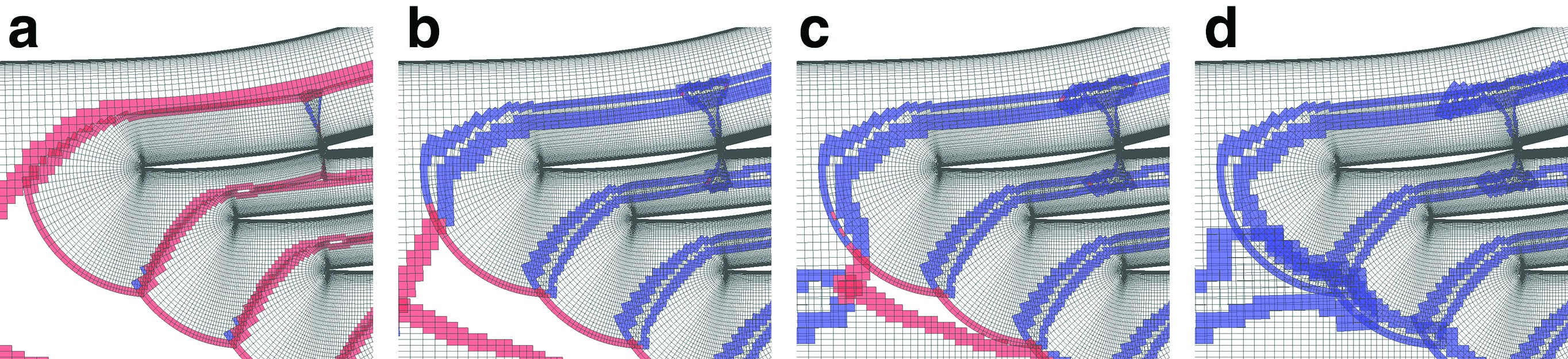
Figure 3 shows the mesh assembly for the present study. The mesh system has two cells in the spanwise direction and 0.75 million cells in total. All the inter-blade passages, bypass channels, and small gaps are successfully connected around the midpoint between the parts. The percentage of activated cells against the total cells is 72.4%.

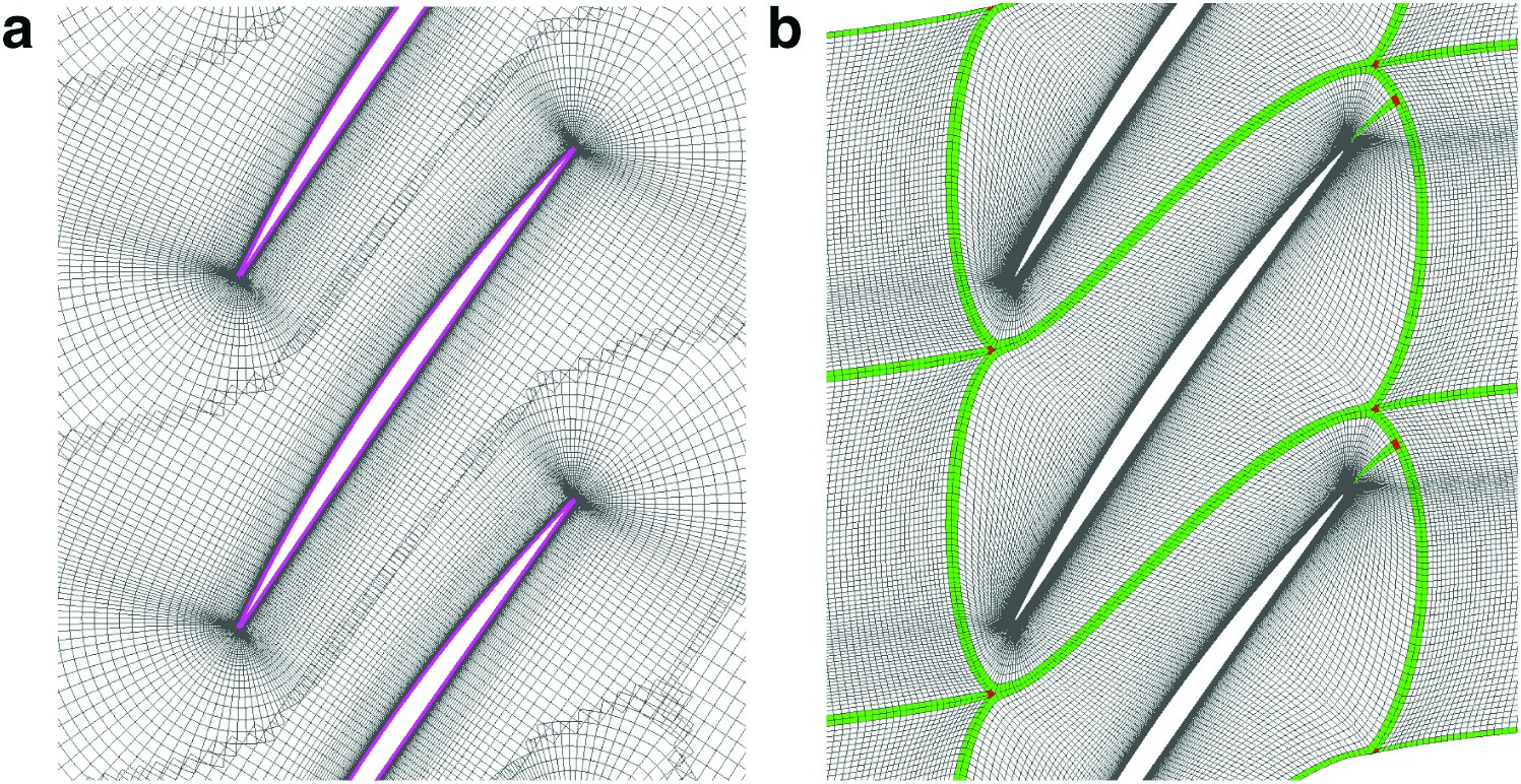
In addition to the wind tunnel mesh, a conventional line-matched multi-block mesh is generated for preparing baseline flow field with perfect pitchwise periodicity. This configuration is referred to as “ideal” case. Figure 4 and Table 2 shows the appearance and mesh parameters for the O-mesh around the blade. The multi-block configuration have slightly higher mesh resolution.
Steady flow results and discussion
Baseline flow field
At the beginning of the discussion part, the baseline flow field for the discussion hereafter is presented for both wind tunnel and ideal configurations. The back pressure for the both cases are 0.67pt. The wind tunnel settings are: θts = 6, θtb = 2.4, θth = 1.2 degrees, and the suction velocity of vs = 6 m/s.
Figure 5 shows Mach number distributions for the both cases. Figure 5 and Figure 5 show the wind tunnel case. The supersonic started inflow is realized for all passages of the cascade and the bypass channel. In the blade passage, the oblique shock from the leading edge and normal passage shock can be observed. The shock pattern including lambda-shaped shock-boundary layer interaction within the passage for the wind tunnel case is quite similar with that in the ideal case shown in Figure 5.
Figure 5.
Mach number distributions for the baseline case. (a) Whole flowfield through the nozzle throat, test section, and downstream the cascade, (b) Wind tunnel configuration, (c) Ideal, infinite cascade.
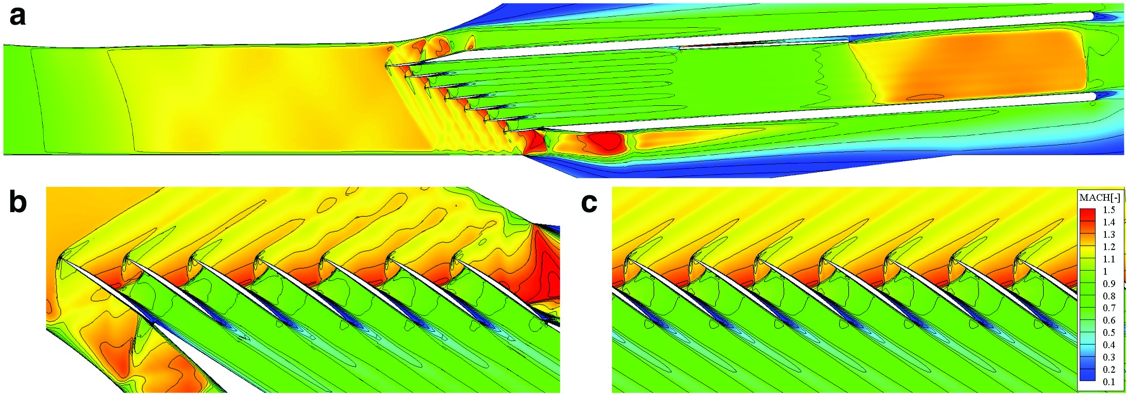
Figure 6 shows Cp distributions on the blade No. −2 to 2 and the ideal case. As expected from the Mach distributions, almost periodic flow field is realized for the wind tunnel case. The positions of the shock are deviated by approximately 5%c within the blade −1 to 2 both on the suction and pressure sides.

Effect of suction on the upstream periodicity
The effect of transonic wall suction is evaluated for making the inflow as uniform as possible. Figure 7 and Figure 7 show comparison of shock pattern upstream the cascade, which is visualized by the horizontal density gradient. The lower bypass is unstarted and significant non-uniformity can be seen in the non-suction case, while appropriate amount of suction gives uniform shock structure as shown in Figure 7.
Figure 7.
Effect of transonic wall suction on the inflow uniformity. (a) No suction, (b) v_s = 6 [m/s], (c) Mach number and flow angle along ML1.
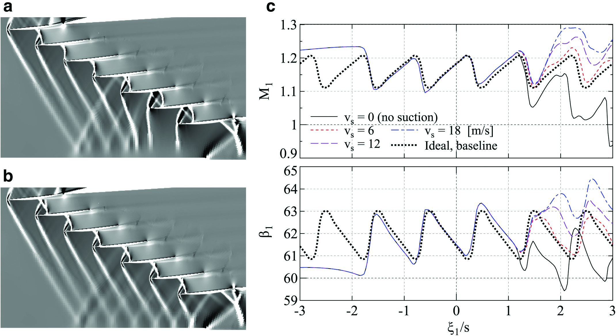
Figure 7 shows detailed comparison of Mach number and flow angle along ML1 against different suction velocities. Both Mach number and flow angle are significantly affected by the amount of suction, and the effect of suction mainly appears upstream the blade 2 and 3. In addition, an appropriate amount of suction gives similar distribution as the ideal case.
Effect of throttling on the downstream periodicity
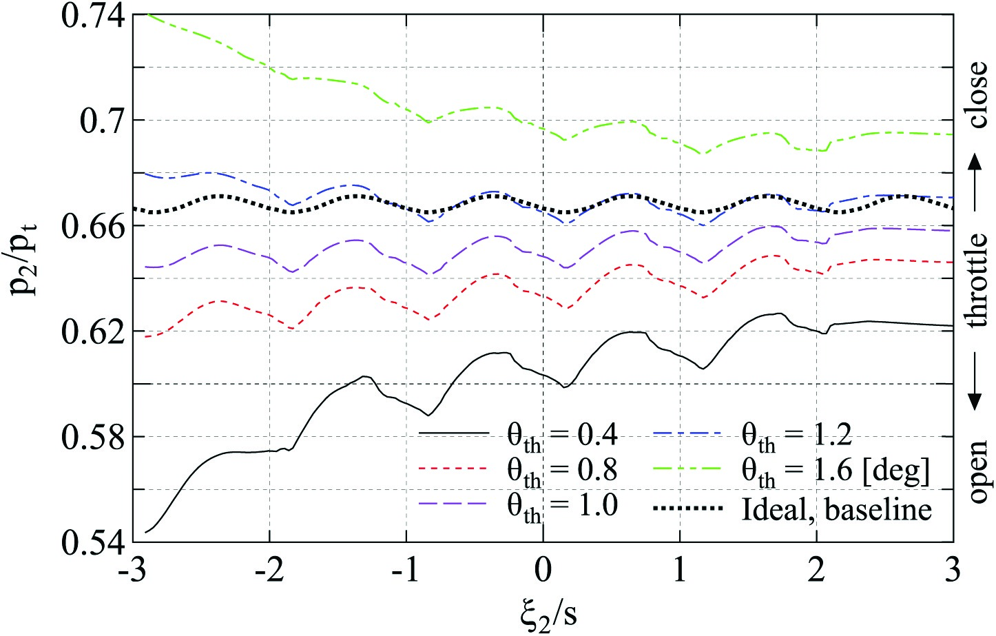
The effect of throttling angle on the downstream periodicity is evaluated by fixing all other parameters. Figure 8 shows a comparison of static pressure distributions along ML2 for five different throttling opening angles: θth = 0.4, 0.8, 1.0, 1.2, and 1.6[deg]. Under the fixed tailboard, the pressure distribution downstream the cascade is highly affected by the throttling angle. For the θth = 0.4 [deg] case, the pressure downstream the blade No. −3 to −1 is significantly small compared to that downstream the blade No. 1 to 3. The situation is opposite for the θth = 1.6 [deg] case.
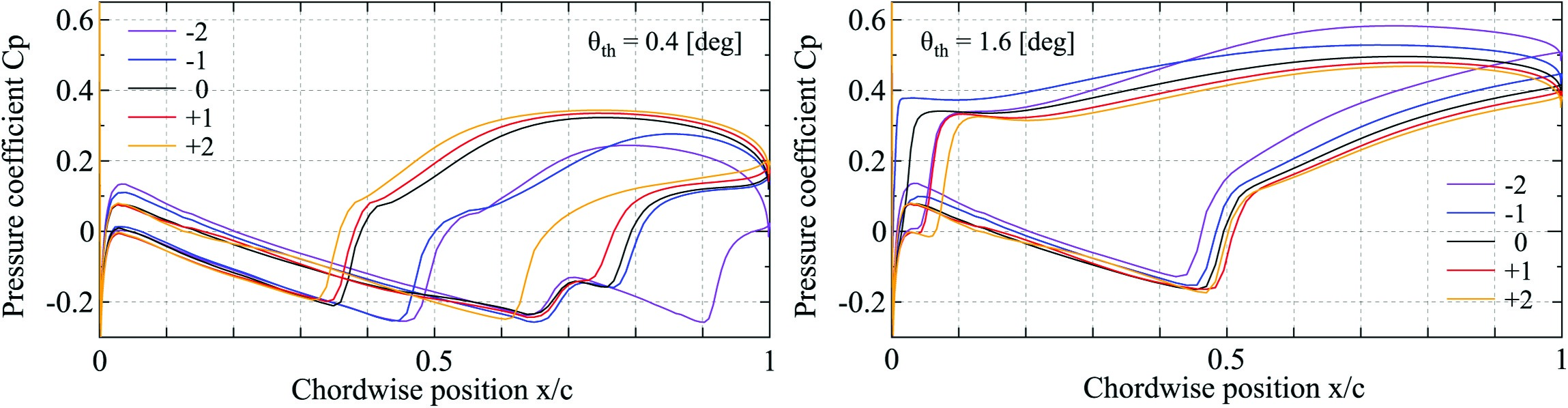
The blade loading is also highly affected by this non-periodic pressure distribution. Figure 9 shows the Cp distributions among five centre blades for the θth = 0.4 and θth = 1.6 [deg] cases. There are significant variations in the blade loading and shock position for these cases, compared to the θth = 1.2 [deg] case shown in Figure 6.
This result is qualitatively consistent with the findings by Lepicovsky et al. 08, and it also implies that there is an optimal throttling angle for realizing the best periodicity for every different tailboard angle.
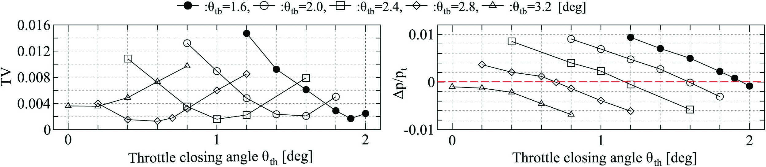
In order to confirm the existence of optimal throttling angle for the best periodicity, the periodicity in static pressure is quantified by parameters Δp/pt and TV in Equations (–). The optimum conditions for these indicators are Δp/pt = 0 and the minima of TV. Figure 10 shows the change in Δp/pt and TV for different tailboard and throttling angles. Each lines are obtained by sweeping θth while keeping θtb constant. The zero-points of the Δp/pt and the local minima of TV can be found on each tailboard angles. Therefore, it can be confirmed that the throttling angle for the best periodicity depends on the tailboard angle.
Controlling pitchwise periodicity and its importance
In the choked cascade with fixed supersonic inflow, all the aerodynamic characteristics are dependent variables of the outlet pressure. Here, the effect of periodicity on the measured aerodynamic characteristics is discussed in detail.
Figure 11 shows the relationships between spatial averaged outlet pressure
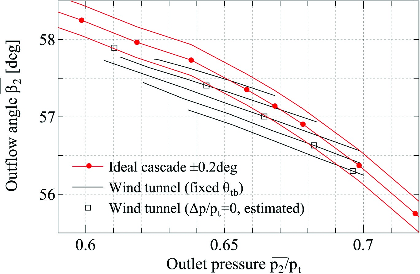
From this result, it can be concluded that realizing the best pitchwise periodicity is quite important for obtaining appropriate aerodynamic characteristics of ideal cascades.
Unsteady flow results and discussion
The AICs are obtained with oscillating the centre blade 06 in both the wind tunnel and ideal configurations. The cascade is operated on the baseline condition shown in the previous section. The wind tunnel computation directly employs the tunnel geometry, while 15 blades are prepared for the ideal case. In order to investigate wide range of oscillation condition, the blade frequency is varied from 50 Hz to 1500 Hz. All the computations are conducted with constant blade amplitude of
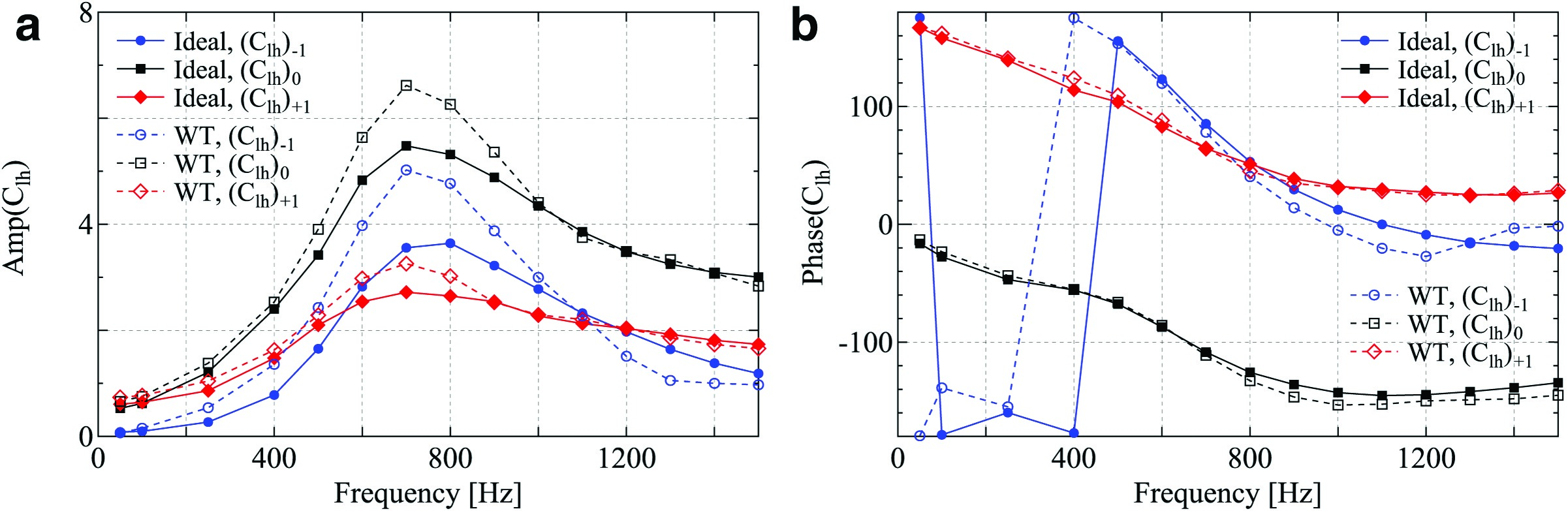
Aerodynamic influence coefficients
Figure 12 shows the comparison of frequency dependency of the AICs on the three centre blades between wind tunnel and ideal configurations. Since the AICs are expressed by complex number, their amplitude and phase angle are shown. The trend of two different configurations are qualitatively similar both in amplitude and phase angle. However, significant difference in amplitude can be seen in the frequency ranging from 400 Hz to 800 Hz, especially for the blade −1.
Blockage effect of the tailboards
In order to find out where the difference in the amplitude of AICs originates, unsteady flow field around the cascade is investigated. Figure 13 shows pressure amplitude around the cascade for both ideal and wind tunnel configurations. Four frequency levels from 250 Hz to 700 Hz are highlighted in order to see the increasing process of the difference.
Figure 13.
Pressure amplitude around the oscillating blade. (a) Ideal, infinite cascade. White line shows tailboard in the WT setup, (b) Wind tunnel configuration.
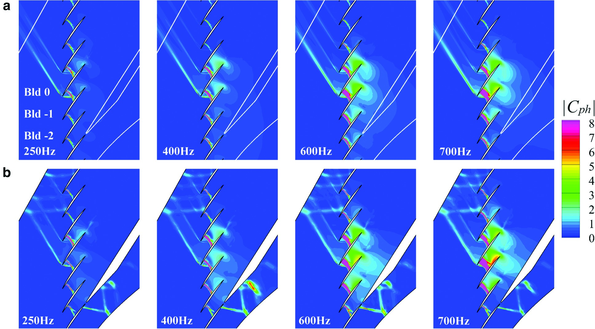
In the ideal cascade shown in Figure 13, pressure amplitude continuously increases at downstream of the blade −2 to −1 as the frequency increases. In other words, the pressure amplitude becomes higher on the downstream of lower blades.
In the wind tunnel configuration shown in Figure 13, the tailboard exists where the pressure amplitude increases in the ideal configuration. Therefore, there can be some interaction between the wind tunnel wall and acoustic wave propagating toward minus-direction of the blade number. The acoustical reflection on the tunnel wall potentially cause the observed amplitude difference. More detailed interaction phenomenon and the consistency with the theoretical backgrounds could not be figured out however, it can be said that the unsteady flow field can be grasped in a qualitative sense by the developed CFD code.
Acoustic cut-on in the duct
Although the actual frequency is very high compared to the past flutter experiments (e.g., up to 550 Hz and 730 Hz for the standard configurations five and seven, respectively [05]), the acoustic cut-on condition in the exit duct appears in the present computation. The lowest cut-on frequency of the acoustic wave propagating upstream and downstream inside a rectangular duct can be derived as follows.
In the present baseline case, the duct width, sound speed and Mach number are D=87.6 mm, α= 327 m/s, and M = 0.693, respectively. The resultant cut-on frequency is
Figure 14 shows the pressure amplitude inside the duct. Figure 14 and Figure 14 correspond to cut-off (1100 Hz) and cut-on (1500 Hz) case, respectively. The pressure amplitude decays toward downstream for the cut-off case, while the wall pressure becomes higher entire in the streamwise direction for the cut-on case. Figure 14 shows the amplitude of wall pressure against blade frequency sampled near the leading edge of the throttle. The pressure amplitude gradually increases as the frequency increases. Then, the amplitude drastically jumps when the blade frequency reaches the cut-on frequency. From this result, it is confirmed that the present method can capture global unsteady phenomena like acoustic cut-on.

Conclusion
A numerical method and its application for an assessment of the flow field inside a wind tunnel was presented. In order to simulate geometrically complex configurations with movable mechanisms, the overset mesh technique was implemented to our structured CFD solver. The mesh of the wind tunnel was created by assembling all the component meshes using distance-based blanking and iterative donor search algorithms. This methodology enabled to simplify the mesh generation and parametric study processes.
Applying the developed method, steady and unsteady simulations including whole the wind tunnel were conducted. The upstream and downstream periodicity of the steady flow field, effect of the tunnel wall on the unsteady flow field, and duct acoustic characteristics were focused on. The findings are summarized as follows.
(1) The periodicity of downstream pressure distribution and blade loading is highly affected by the setting of tailboard and throttle. An optimum throttle position for the best periodicity exists for each tailboard angle, which provides appropriate aerodynamic characteristics of ideal cascades in the wind tunnel environment.
(2) The difference in the AICs between ideal and wind tunnel configurations becomes large when the pressure amplitude increases on the downstream of lower blades.
(3) The present method can capture global unsteady phenomena like acoustic cut-on.
The developed CFD solver will be helpful for future design activities or assessments of flow field inside various experimental facilities.
Nomenclature
β
[deg]
flow angle relative to the cascade
θts
[deg]
setting angle of the test section relative to the horizontal line
θtb
[deg]
setting angle of the tailboards relative to the chordwise direction
θth
[deg]
opening angle of the throttle relative to the tailboards
θs
[deg]
stagger angle
ξ
[m]
coordinate on the measurement line
α
[m/s]
sound speed
c
[m]
chord length
Cl
[-]
steady lift coefficient
Clh
[-]
unsteady lift coefficient
Cp
[-]
steady pressure coefficient
Cph
[-]
unsteady pressure coefficient
D
[m]
duct height downstream the cascade
f
[Hz]
frequency
[m]
oscillation amplitude of the blade 0
l
[m]
span length
M
[-]
Mach number
n
[-]
direction vector normal to the chord line
pt
[Pa]
total pressure
S
[m]
pitch length
T
[sec]
time period of blade oscillation
t
[sec]
time
vs
[m/s]
suction velocity on the transonic wall
x
[m]
chordwise distance from the leading edge