
Introduction
In recent years the idea of digitalizing the design process for gas turbines is becoming more common, in order to move towards the so called Industry 4.0. What is not clear is how to achieve this, what is needed and how to produce a design that is truly driven by recent digital development. The overall goal of this work is to breakdown all the building blocks needed to achieve this.
In design and optimization there are three aspects that are inherently interconnected: manufacturing method, optimization strategy and estimator (accuracy, speed, formulation). In terms of manufacturing, the rapid development of Additive Manufacturing (AM) technologies over the past 30 years has enabled levels of complexity in the manufacture of structural components never achieved before. The gap between the increased manufacturing flexibility and traditional design methods highlights the necessity of new design approaches. The potential of automated design methodologies makes them effective design tools, capable of designing optimally loaded, intricate components to manufacturable standard, while fully exploiting the current manufacturing capability.
As for optimization, design techniques based on numerical optimization have been developed since the 1970s and have evolved from Size Optimization to Shape Optimization and, most recently, to Topology Optimization (TO). Topology Optimization defines a truly free optimization, where even the topology of the geometry is not a priori defined, but only the objective goals and constraints. It is also called functional driven optimization because the main driving parameter is the functionality of the component (Bendsøe and Kikuchi, 1988; Bendsøe, 1989). The approach gained traction in structural Topology Optimization, while Fluid-structure Topology Optimization (FSTO) remains under development (Pietropaoli et al., 2018). In structural optimization, Topology Optimization methods are the current state-of-the-art in automated design methods, capable of determining the solid material distribution in space that optimally satisfies boundary conditions and design constraints without the need for an a priori definition of structural shape. Such techniques are highly valuable in high-performance engineering applications where the minimization of structural mass is critical in the pursuit of efficiency and performance. Their successful utilization in the aerospace industry can drive significant weight-saving and reduced design times by producing optimal designs with high structural efficiency to manufacturable standards. A high structural efficiency is of paramount importance in the design of high-performance components, as all solid regions are effectively utilized in the process of load transmission. Such structures are particularly important to the aerospace industry, where the minimization of weight is critical to ensure compliance with strict emissions regulations. Regarding FSTO, two main methods have been discussed in literature, Level Set Method and Adjoint Based Optimization (Gaymann et al., 2019a,b). Lately machine learning methods based on Deep Neural Networks have been presented (Gaymann and Montomoli, 2019). Adjoint based and Deep Neural Networks will be discussed in this work.
Considering estimators, there is a strong debate in the literature about the accuracy of the current estimators used for optimization: if the estimator is not accurate, how can the optimized geometry be a real optimum? (Hammond et al., 2020). This question is connected to the optimizer. If an equation is very complex, or if a neural network is used, it may be very difficult to define an adjoint formulation to the design process.
There is not a single work showing the application and limitations of the design of gas turbine components discussing these aspects. This work will start showing topology optimization methods applied to gas turbines, with structural and fluid topology optimization impacting different areas. In particular we believe that structural topology optimization is important in cooled rotor blades and low-pressure turbine blades, where centrifugal forces are dominant. Fluid Topology Optimization will instead play a key role in high pressure turbine components to redesign the internal coolant system.
Afterwards the paper highlights how recent development in machine learning can be used to increase the accuracy of the estimators. Two methods are highlighted, Gene Expression Programming (Hammond et al., 2020) and Deep Neural Networks (Frey et al., 2020). Finally, an innovative approach is shown (Gaymann et al., 2019a,b), directly leveraging Deep Neural Networks to design any component.
The methods presented in this paper have been validated in several other works as presented in the reference list. The overall goal is to provide the reader with an overview of the available methods which are enabling the shift towards a fully digital design of a gas turbine.
Structural topology optimization
Structural Optimization is the application of constrained mathematical optimization methods to the design of structurally efficient solid structures. It involves the definition of an objective function to be maximized or minimized and a set of design constraints, typically restrictions on the maximum volume of available material. In this section, two types of topology optimization methodologies are considered to optimize gas turbine components: Solid Isotropic Material with Penalization (SIMP) and Sequential Element Rejections and Admissions (SERA).
The Solid Isotropic Material with Penalization (SIMP) method is a subset of the Density-based family of TO methods, which employ a continuous design function to quantify the stiffness tensor in space. Originally proposed by (Bendsøe, 1989) and later by (Zhou and Rozvany, 1991) the SIMP method introduces a penalization factor p (where p > 1) and formulates the material stiffness tensor as shown in Equation (1).
where
The Sequential Element Rejections and Admissions (SERA) method belongs to the Biologically inspired family of TO methods, where a structural performance threshold is used to determine the retention and rejection of structural elements. It was first proposed by (Xie and Steven, 1993) and named “Evolutionary Structural Optimization”, a term which was criticized in literature because, in the field of computational optimization, the label “Evolutionary” is used to denote population-based solvers such as Genetic Algorithms. In this paper, the authors refer to the method as SERA, as originally suggested by (Rozvany, 2001). The method is based on the rejection and admission criteria, determined by the structural performance of each element relative to a pre-determined threshold. Elements not meeting the threshold are assigned a low-magnitude elasticity modulus and those that do are assigned the solid elasticity modulus. For example, using a Von-Mises stress criterion the rejection and admission criteria would be formulated as shown in Equations (2) and (3) respectively.
RR and IR denote the Rejection Ratio and Inclusion Ratio respectively. The thresholds are shifted by updating RR and IR and the process is repeated until a global structural performance target, such as elemental stress level or specific stiffness, is achieved. In this study, the optimization algorithm proposed by (Zuo and Xie, 2015) is used.
In this study, compliance was used as the objective function. As it is a measure of the elastic strain energy stored in the material by virtue of its force-induced displacement, maximum stiffness can be achieved by minimizing the compliance objective function. The complete formulation of the optimization problem is illustrated in Equation (4).
In the above equation, the compliance matrix is denoted by C(X), where X is a vector of the element design variables that take the value xi = 1 for solid elements and xi = xmin for void elements. F = KU represents the equilibrium constraint for linear elasticity where F, U are the force and displacement vectors respectively and K is the stiffness matrix. V(X) is the total volume of the structure which is defined by the available material volume V*, where 0 < V* < 1.
In gas turbines, there are two areas where structural/topology optimization can have a strong impact:
High pressure turbines, to remove material in the rotor blades, reducing centrifugal forces and startup time. The optimization minimizes the weight and control both stresses and thermal gradients. Until few years ago weight reduction was mainly associated to aircraft engines. In recent years, the electric grid requires gas turbines with fast startup and shutdown to cope with the variations introduced by renewable sources. For this reason, weight reduction is also important.
Low pressure turbine blades. The low pressure turbine is representing the heaviest part of aircraft engines and it can benefit from weight reduction.
Two test cases are shown here, C3X, as a cooled rotor example, and T106C, being representative of a low pressure turbine blade. Take-off conditions were assumed throughout the analysis, with angular velocity of 12,400 rpm. The total blade mass was assumed to be m0 = 300 g and the mean radius from the centre of rotation was set at rm = 0.216 m.
The gas pressure on the turbine blades was accounted for using the experimental values of (Chana and Jones, 2003) resulting in a pressure difference across the row of ΔPs = 316 kPa. The blade material selected for use in this study was Grade 310 Stainless Steel, due to the requirement of a solid isotropic material for the optimization algorithm. The material properties used are shown in Table 1 and all values used in this study are representative of a HPT. The results are shown in Figure 1.
Table 1.
Material Properties of ASTM 310 stainless steel.
| Property | Value | Unit |
|---|---|---|
| Density | 8,000 | kg/m3 |
| Elasticity Modulus | 200 | GPa |
| Poisson’s Ratio | 0.30 | [−] |
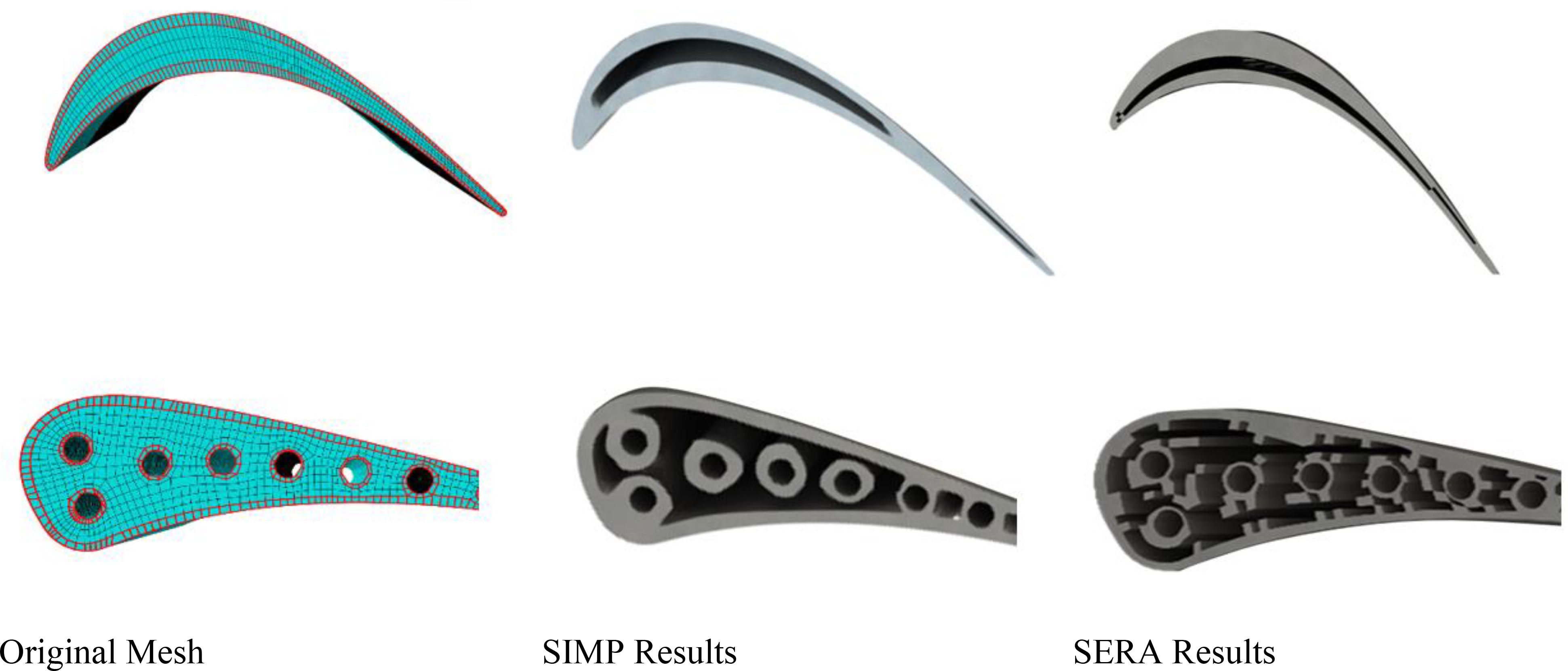
In these two cases it is observed that SERA generates geometries that can outperform SIMP results. SERA geometries are more intricate even in cross direction. The objective function used in both cases were compliance. For the same external shape, SERA obtained 36.7% lower compliance for T016C and 22% lower compliance for C3X compared to SIMP. However, SIMP can generate smoother solutions which may have an advantage from a manufacturing point of view. In the picture below SIMP and SERA results are shown for T106C and C3X profiles where the two profiles are optimized keeping the external shape constant and the internal coolant ducts untouched.
Fluid structure topology optimization
The core idea of Fluid Structure Topology Optimization (FSTO) is to find the optimal solid design of a component by emulating a natural process of sedimentation, where the optimization objectives themselves are based on the flow of fluid through the component. The domain is assumed to be a porous medium with a space dependent design variable, impermeability. The optimisation consists of an iterative process by which the impermeability is updated to meet the prescribed objectives while respecting a set of constraints. At the end of the process, the distribution of impermeability within the domain identifies which region is solid and which one is occupied by the fluid. The process, as in this paper, requires the definition of the following:
Design Domain
Impermeability
The vector of state variables X, identified in this work as the set of p pressure, v velocity vector and T temperature.
The multi-objective function F. This is a function of the state and design variables
Constraints R, equalities and inequalities that X and
The set
The solution
where, in this case, the function “
with
where
where the Lagrangian multipliers q, u and
and the steepest descent algorithm is used to iteratively search for this solution,
where
In this work, the solver TOffeeAM is used to show the application of FSTO for different objective functions crucial in the design of gas turbines. These are:
Stagnation pressure loss minimization
Ducts with a diodicity behaviour (valves without parts)
Heat transfer and pressure losses (multi-objective)
Detailed explanations of these application are shown in (Gaymann et al., 2017; Pietropaoli et al., 2018) and a brief overview will be presented here. For stagnation pressure loss optimization, the return channel used by (Vestraete et al., 2013) is used. On the test case shown in Figure 2, different inlet velocities are used to obtain each solution. The variational approach allows generation of vanes inside the u-bend, which can vary in both number and shape. It is this possibility of altering the solutions topology that is the key advantage over shape optimisation techniques shown in (Vestraete et al., 2013), in which introducing solid material inside the domain, disconnected from the external boundaries, is not possible unless proper geometry parametrizations are considered beforehand.

FSTO can also be applied to consider a domain with different flow directions. For example, we can consider a flow with low pressure losses in one direction (forward flow) and high pressure losses in the other (reverse flow). In this case the resulting geometry is a static device acting as a valve, or a valve without moving parts. In this case, a single optimization parameter is considered, known as diodicity. Figure 3 shows solutions for flow through a chamber with varying levels of diodicity in which manufacturability constraints such as minimum passing area have also been considered.

Results are compared to geometries already given in the literature for a 2D topology optimisation, obtained with a different method. The formulation used by (Gaymann et al., 2018) and shown in this work has two advantages compared to other methods: it is able to generate inherently tree dimensional shapes and it is stable for a Reynolds numbers close to the ones characteristic of secondary air flow systems. The valve example also shows another capability of FSTO: the ability to translate a system made of multiple parts (a standard valve) into a single static component. The advantages to this are numerous, not least including the inherently reliability of the system.
A similar approach can be used to include heat transfer effects during the optimization phase. In this case the energy equation needs to be introduced into the optimization process. A full description of the optimization method is described by (Pietropaoli et al., 2019). In Figure 4 the three dimensional optimization of a channel with heat transfer is shown.

What is interesting here is that the solver is able to find a periodic solution along the main axis along the flow direction, without this being imposed. Furthermore, the code tends to develop a rib like structure for this specific Reynolds number. For different flow configurations the solver is capable of generating completely different structures.
This concludes the discussion on the current state of FSTO within the group however a key problem with FSTO currently is the accuracy of the estimator (the CFD solver) which is based on RANS turbulence treatment. It seems clear that using a suboptimal estimator will likely lead to the generation of suboptimal solutions. To tackle this problem the group has been working on different Machine Learning approaches which enable improvements in the accuracy of RANS solvers with a view to implementing these within the FSTO framework.
Machine learning and topology optimization
As mentioned, the drawback of FSTO and all RANS based estimation is the inherently inability to capture accurately the objective function (pressure losses, heat transfer). Conversely it is not possible to use DES simulations (or any higher fidelity methods) for FSTO, mainly due to the computational cost and the unsteady terms in the adjoint equations.
Three Machine Learning methods have been studied to overcome this problem:
Gene Expression Programming applied to High Fidelity Simulations (Hammond et al., 2020)
Neural Networks for Turbulence Closure (Frey et al., 2020)
Monte Carlo Tree Search and Deep Neural Networks (Gaymann and Montomoli, 2019)
The first two methods use a similar strategy: by using high fidelity simulations, develop RANS closures to obtain RANS simulations with higher accuracy. When compared to Neural Networks, Gene Expression Programming has the advantage of developing an explicit equation. The equation is easily understood by researchers and it is possible to analyse the behaviour of all turbulence terms. A further, and equally relevant advantage is the computational time. Knowing the equation allows the programmer to include the most efficient version in the solver.
However, although Neural Networks hide their resulting equations (especially when Depp Neural Networks are used), they are far more flexible and allow highly non-linear behaviour. Recent work by (Frey et al., 2020) however, has shown that a relatively lean network is able to capture the majority of the features in turbomachinery flows.
The final method presented in this work leverages machine learning capabilities even further (Gaymann and Montomoli, 2019). The researchers used Artificial Intelligence to build two concurring Neural Networks, which play an optimization game based on a Monte Carlo Tree Search. The score of the game is based on aerodynamic performance and the work proved that this approach is suitable for geometrical optimization problems.
Gene expression programming
Gene Expression Programming (GEP) is a symbolic regression method, aimed at identifying the best constitutive relationship from data. In this formulation, the data are high fidelity CFD simulations (DNS and DES). Compared to other fitting strategies where the “shape” of the underlying function is a priori selected and the weights of the bases are modified by the regression, GEP allows the code to build an equation based on a library of available functions. Usually these are represented in a parse tree formulation, where for example, an equation is translated into a graph. In Figure 5 we comparing the results of GEP against different models applied to the complex topology optimized geometry described in (Pietropaoli et al., 2019). The picture shows the anisotropy error against DES data, plotted for a standard linear model, a nonlinear closure from (Wallin and Johansson, 2001), a simple global regression and GEP.
Figure 5.
Comparison of Anisotropy Square Error with different closures and GEP, scale 0–1 over each slice.
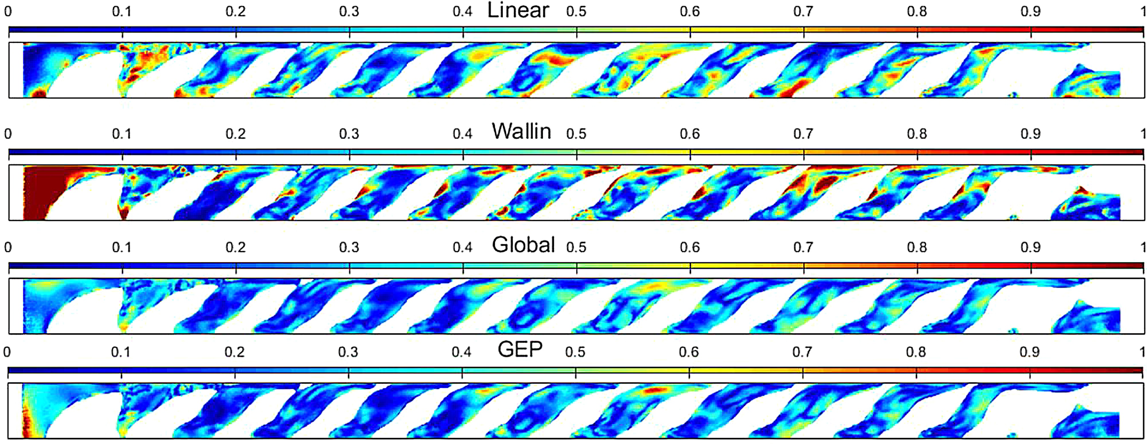
The major differences are near the inlet which explains the decision to perform regressions based on specific flow regions in subsequent investigations. GEP does not only allow good local representation of anisotropy and a-posteriori tests with the GEP formulation have yielded a better mass flow prediction when compared against both (Wallin and Johansson, 2001) and the global regression. Another advantage is that the turbulence closure obtained in a complex geometry like the one used here is applicable to other test cases, still outperforming other turbulence closures. For example (Hammond et al., 2020) applied the closure to a back facing step and found an improved prediction of the velocity field over a standard linear model when comparing to DNS data.
Neural networks
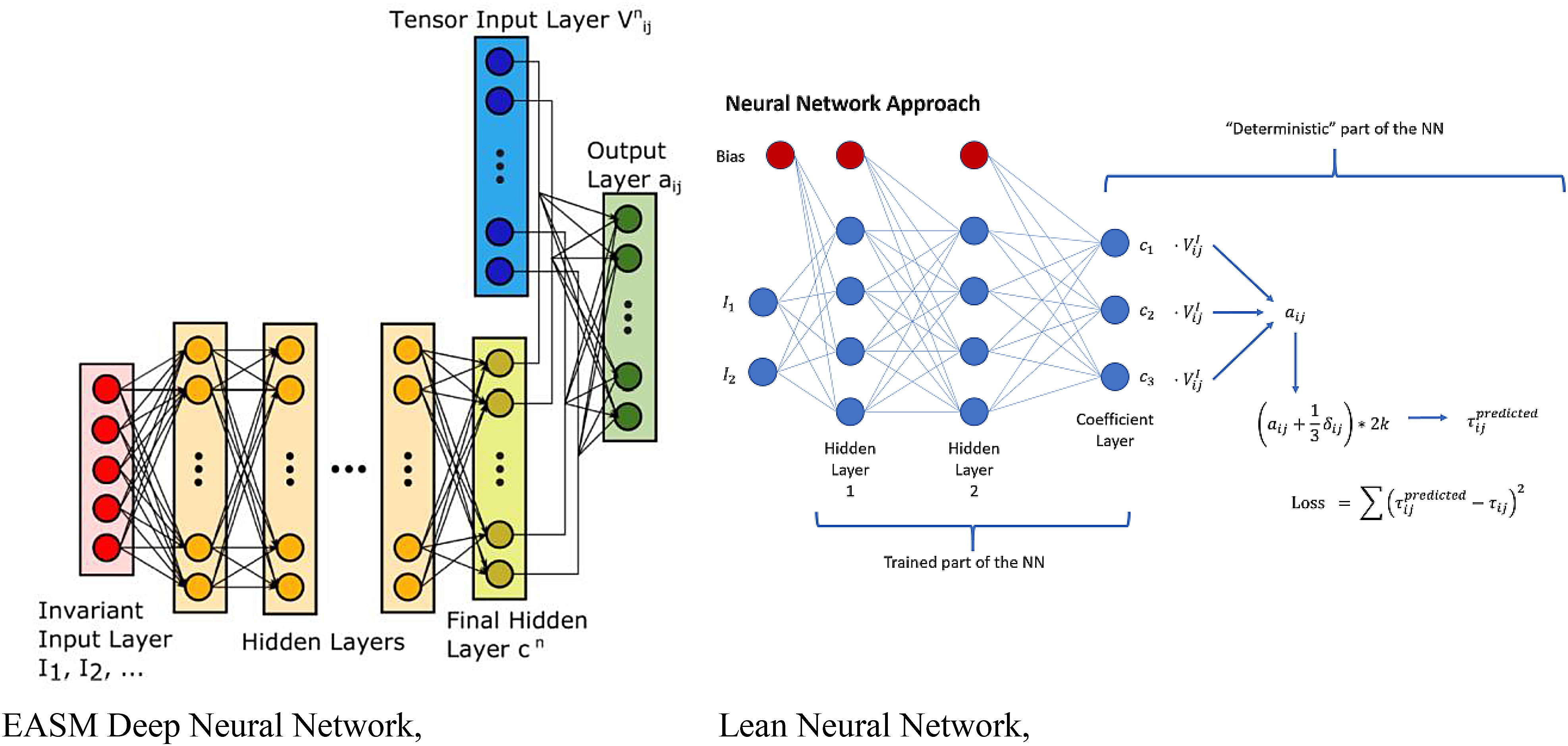
In data-driven turbulence closures using Neural Networks, different network topologies can be used, to achieve different accuracy or to mimic the behaviour of the turbulence closure itself as shown in Figure 6.
When training a DNN on high fidelity data, the goal is to learn the closure which provides the best fit in every turbulent region. Because of this, including regions which do not experience any significant turbulent intensity will negatively impact the predictive performance and convergence of the DNN. There are different methods than can be used to select the training points:
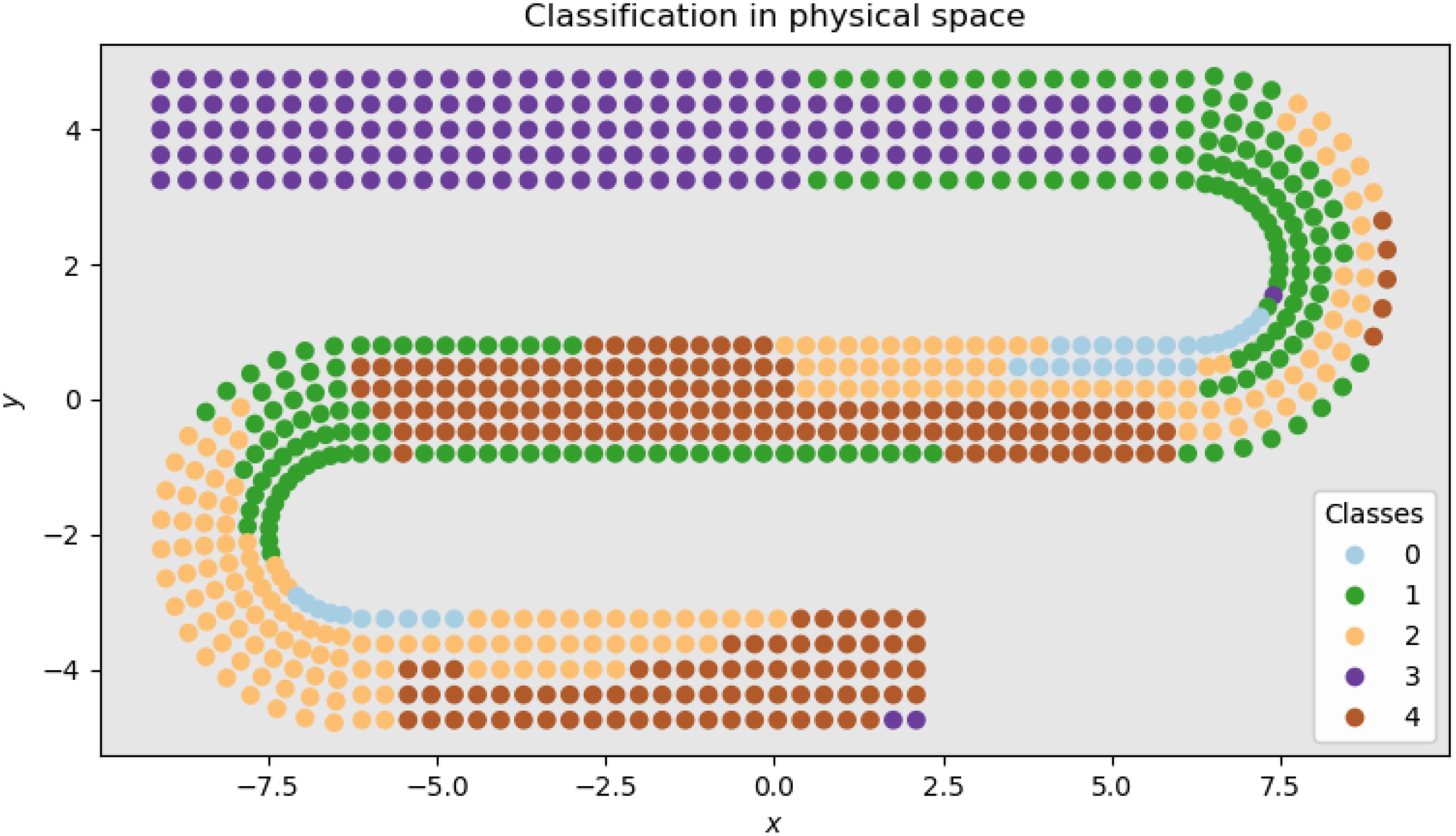
Classification algorithms. As shown by (Alvarez De Toledo Ortiz, 2020; Frey 2020), it is possible to classify different flow regions, based on turbulence level, pressure gradients etc as shown in Figure 7. The flow in the figure below is classified identifying for example, the separation region (0).
Define a priori a threshold level of TKE. Here only those points which experience a high TKE level are used in the training phase, Isaksson (2020).
To define the Neural Network it is important to define the optimizer learning rate, number of hidden layers, number of neurons, activation function and dropout rate. An extensive study of network topology on the predictions of fluid dynamics has been done by (Gaymann et al., 2019a,b) by optimizing the network topology to improve the data fit. They found that even with very simple neural networks, capturing of highly non-linear behaviour was possible.
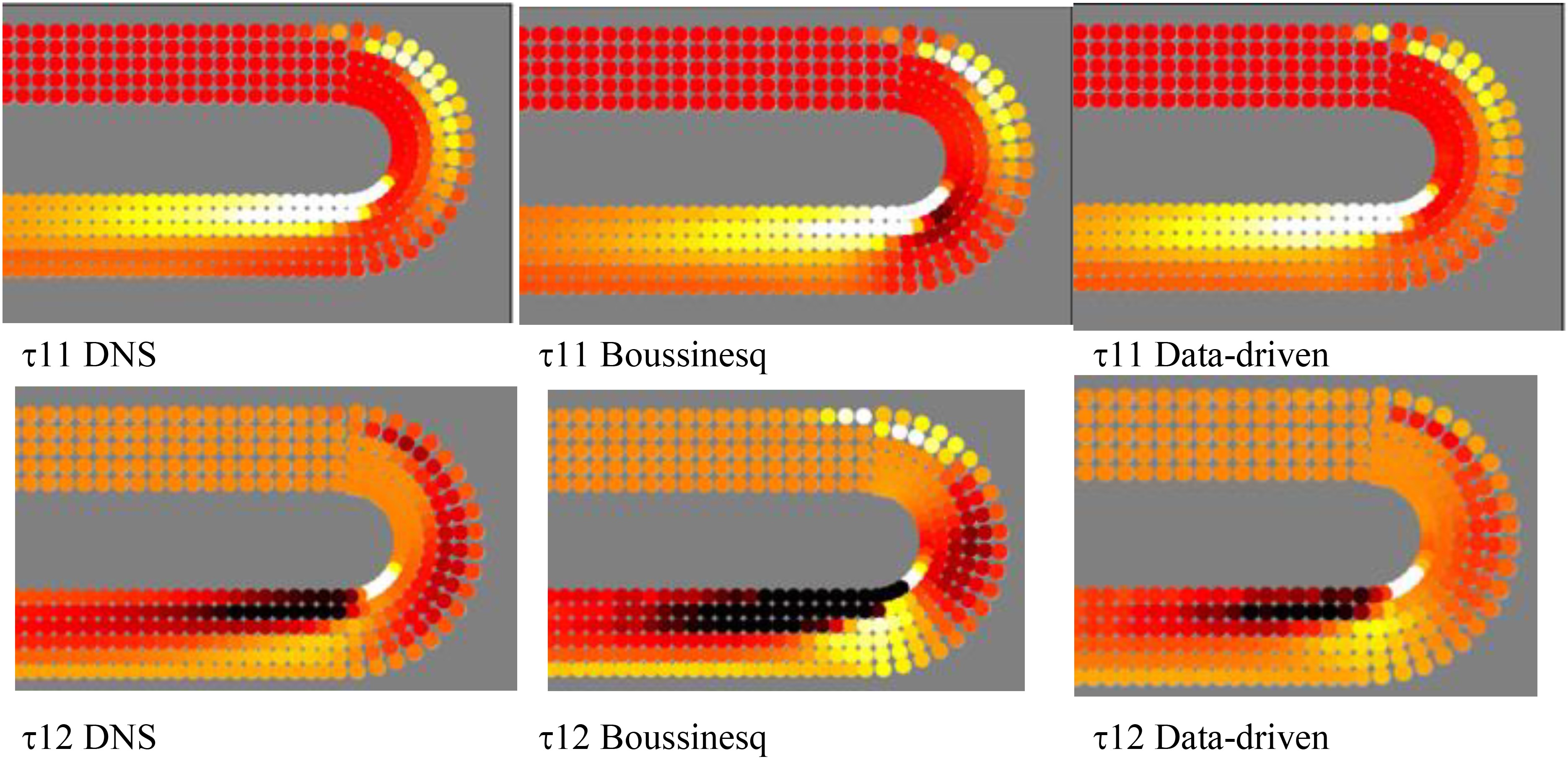
Both GEP and DNN approaches outperform standard k-ω models. Figure 8 shows the comparison between DNS simulation, standard Boussinesq approximation in k-ω models and data-driven models. The data-driven formulation has a similar accuracy than DNS results with 3 orders of magnitude less computational effort.
Monte Carlo tree search with deep neural network
Recent development in machine learning has opened the possibility of using Deep Neural Networks for design. An interesting work has been shown by (Gaymann and Montomoli, 2019), mimicking applying recent developments in game and AI technologies to design. The work used the Google Go algorithm, assuming that a design space is similar to a Go board, where white elements are the fluid part and the black elements are the solid one. Instead of using the rules of Go to design, the researchers used the aerodynamics pressure losses as the objective of the game. The method is fully general however, and any engineering approach can be used. Here the research has been applied to Fluid Structure Topology Optimization.
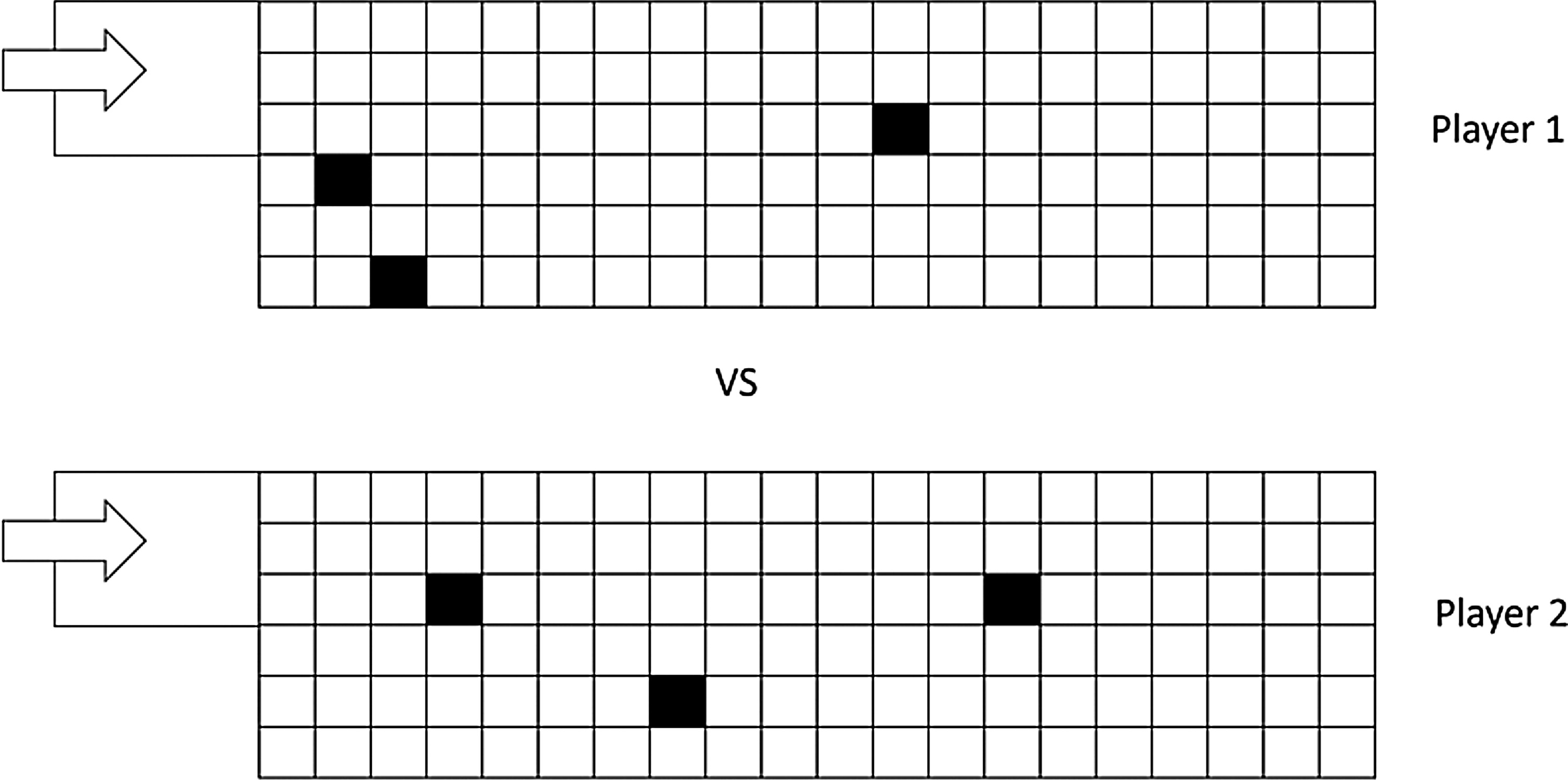
The game starts as shown in Figure 9, where the two players add solid (black cells) to the board full of fluid (white cells).
The players are not aware of, nor do they have any previous knowledge of the topology optimization problem. For each configuration, a CFD solution is obtained and the “score” is evaluated by the aerodynamics performance. After few iterations, the two players are able to find the solution that minimizes losses in the classical back-facing step geometry as shown in Figure 10.

The advantage of this approach is that any estimator can be used, even DNS, without the need to modify the estimator structure to “play” this optimization game. Moreover, the authors have modified the Google Go algorithm to allow a machine to play against itself and all standard visual algorithms to increase the mesh resolution can be used to increase the mesh size and the accuracy.
Conclusions
The paper presents recent developments from the Uncertainty Quantification Lab of Imperial College of London in the field of Digital Design of a Gas Turbine. The application of the in-house solver for Fluid Structural Topology optimization is able to obtain geometries that are more efficient than today’s gas turbine components. Furthermore, we have shown that digital design can replace not only component design, but can also simplify the system as shown by the generation of valves without moving parts. Computationally, the formulation used is about 20 times more efficient than standard shape optimization, while outperforming the performance of the final component.
Different optimization strategies have been presented. In structural topology optimization, two algorithms are compared, SIMP and SERA. While SERA outperforms SIMP as in terms of raw objective value, the geometries produced are very intricate and less smooth than the results generated by SIMP.
With regards to fluid topology optimisation, the accuracy of the estimator (CFD solver) is crucial. Three different methods are presented, two leveraging high-fidelity simulations (with GEP or Neural Network) and one using a Monte Carlo Tree Search strategy. Both GEP and Neural Network strategies outperform standard RANS closures, allowing the estimator to have an accuracy in the order of DNS or DES. The Monte Carlo Tree Search approach is instead able to use directly higher fidelity methods within the optimization process, suggesting a completely different strategy for the future.