
Introduction
The solving of engineering problems often relies on a combination of deductive logic and the engineer’s intuition. While deductive reasoning can be formalised and taught in a reproducible manner, intuition is acquired through personal experience. The reliance on personal experience, however, implies accepting personal bias. This is undesirable if reproducible and objective decision-making is required. Typical scenarios where this is the case comprise the area of quality assurance and the diagnosis of engine defects in Maintenance, Repair, and Overhaul (MRO) applications.
Automation of diagnostic processes reduces the impact of personal bias significantly. While this benefit may be limited in some cases where a defect causes a direct, local, and measurable “symptom” – e.g., a measurand exceeding a clearly defined threshold – it is certainly not negligible if the presence of a defect is to be inferred indirectly from global quantities or downstream flow distributions.
Such indirect diagnostic methods are of great economic interest for MRO service providers and airlines because they can reduce unnecessary disassembly and, hence, ground time of the serviced engine. Here, the inference of hot-gas path defects from analysing the exhaust jet of an engine presents an exemplary use case. The defects are identified by classification of these exhaust density fields for defects which are expected to occur.
Artificial Intelligence (AI) or, in this case more specifically, Machine Learning (ML), provides a rich toolbox for approaching this and similar virtually intractable problems by combining algorithmic problem-solving with formalised ways to gather, store, and extract experience-based decision criteria while minimising the amount of necessary assumptions.
The use of AI for condition monitoring of aircraft engines or gas turbines is already part of some investigations. In particular, Artificial Neural Networks (ANN) and Support Vector Machines (SVM) are often used as robust approaches to classification problems for an automated detection of events. Cumming (1993) used a neural network to monitor the condition of aircraft engines. He was able to show that neural networks also can be used without supervised learning and can potentially improve engine monitoring. Yildirim and Kurt (2018) successfully used ANN for the prediction of the exhaust gas temperature based on real flight data in order to identify power losses of aircraft engines.
SVM have also been used frequently for monitoring the condition of aircraft engines and stationary gas turbines. A comprehensive overview is provided by Widodo and Yang (2007). Wang et al. (2012) have used the SVM approach to create a bug detection-system, which can be used for off-line maintenance applications and on-line monitoring during flight. Hayton et al. (2001) and Hayton et al. (2007) used an SVM algorithm to detect anomalies in the vibration spectra of engines. Kim et al. (2012) combined ANN and SVM to detect defects in aircraft engines.
The results of the investigations showed that both algorithms are suitable for monitoring the performance of gas-turbine engines automatically. Finally, Zhou et al. (2015) compared the performance of SVM and ANN for defect detection in a gas turbine. Their results indicate a better performance of SVM, especially when smaller data sets are used for training. This conclusion was confirmed by Zhao et al. (2014) who used an SVM algorithm for the prediction of the age-related performance loss in aircraft engines.
A further advantage of SVM is that these algorithms can be used not only for conventional pattern-recognition problems, i.e., the classification of data sets into predefined classes, but also for the detection of anomalies, as shown by Matthaiou et al. (2017). Thus, it is possible to detect deviations from the reference state of an engine by identifying outliers. This possibility expands the area of application of SVM significantly to unexpected or previously unknown defects.
Motivated by the economic potential and the potential to provide accurate and reliable engine diagnosis, this paper investigates the automated detection of hot-gas path defects using an SVM algorithm to evaluate exhaust density fields of an aircraft engine. These density fields can be captured experimentally using the Background-Oriented Schlieren (BOS) method (see Goldhahn and Seume, 2007; Raffel, 2015) which yields a cross-sectional density distribution based on the local variation in the refraction index.
The suitability of SVM for automated defect detection is analysed by using the density fields obtained from BOS measurements in two individual test cases. Experimental combustion chamber measurements, where a defect was introduced by varying the local power of individual burners in a combustion chamber provide the first test case. These experimental results are used to define integral parameters for the SVM evaluation. These parameters are transferred to a second test case which comprises numerical simulations of the hot-gas path of a real aero-engine. Here, defects were introduced in the numerical model and synthetic BOS measurements were conducted in the exhaust jet. Both test cases provide a suitable data set for training and validating the SVM. The assessment of this combination of density-distribution measurements with subsequent SVM evaluation answers the following key questions:
Can individual defects in the hot-gas path be detected via reconstruction of the characteristic density field?
Can this defect detection be reliably automated using Support Vector Machine algorithms?
Is the automated defect detection capable of distinguishing between individual defect mechanisms without creating false positives?
Methodology
The methodology applied in this paper is the same as devised by Hartmann (2020).
Background-Oriented Schlieren method
Optical measurements, such as the background-oriented Schlieren method (BOS), are particularly suitable for machine-learning based evaluation as they yield a robust reference case to which variations can be compared. BOS measurements are also comparatively easy to conduct, as they require only a simple test setup and no complex optical equipment or lasers. Raffel (2015) gives a detailed overview on the BOS measurement technique and its applications.
BOS measurements have been successfully applied in aero-engine applications. Politz et al. (2013) were able to visualize the exhaust jet of an aircraft during take-off while Schroeder et al. (2014) added a reflective surface for higher quality images.
A brief overview of the physical principles behind BOS measurements as detailed by Hartmann (2020) is given in the following. The method is based on the deflection of light rays passing through an optically inhomogeneous field. The deflection angle
where
The Gladstone-Dale constant K is unique to the fluid investigated. With these equations, a direct correlation between the deflection of a light ray and local density gradients can be formulated. Using a comparatively simple setup consisting of several cameras directed towards a background with a unique pattern (e.g., point-dotted), a two-dimensional density field is measured: First, a reference picture of the background without any flow is captured. This measurement is then repeated with the flow to be investigated present. The light ray deflection due to inhomogeneities in the flow field cause a displacement in the background pattern. This displacement can be cross-correlated by comparing the reference picture and the picture with flow present.
To reconstruct the density field, a tomographic reconstruction algorithm is required to obtain the multi-dimensional density distribution from the integral deflection angles across several cameras. The algorithm detailed by Hartmann and Seume (2016) is used for reconstruction.
In this work, both experimental BOS measurements and synthetic measurements based on numerical simulations are considered. For the numerical simulations, synthetic BOS measurements are performed with the methodology presented by Adamczuk et al. (2014). This methodology uses numerical simulations of the exhaust jet to calculate the deflections that would be measured with BOS for a given tomographic set-up. The synthetic measurements are used afterwards to perform the tomographic reconstruction with 32 virtual cameras. A random measurement noise of ±0.1 pixels is added to the synthetic measurements. This noise accounts for the typical accuracy of the block matching algorithms used to calculate the pixel displacement on the background. For each numerical simulation, 75 synthetic BOS reconstructions are performed. These are used for the automatic detection of defects using the Support Vector Machine (SVM) algorithm explained in the following section.
Support Vector Machine algorithms
SVMs are supervised learning models and the algorithms are originally designed for the classification of two-class problems. The starting point is a training data set, which contains data with two known class affiliations. The main basics of the SVM results from linear separation of data sets and is then generalised. This logic is common and described by Niemann (1983) and Müller et al. (2001) among others.
Based on the separation logic and a training data set, the SVM algorithm constructs a hyperplane between the classes to separate them. After this training procedure, a new testing sample can be classified based on this hyperplane into one of the classes. SVM algorithms are designed to separate both classes. This is achieved by maximizing the margin between the nearest points of both classes. The data points which are used to define the hyperplane are called support vectors. Once the support vectors are defined, the origin data are no longer required, because the interpolated support vectors include all necessary information to define the classifier. The derivation is thus initially only valid for linearly separable data sets. This is rarely correct in real-world applications since the samples often overlap to a certain extent. To be able to classify such data records with a SVM as well, slack variables are introduced, which prevent a violation of the conditions. They allow a certain number of outliers in the training data.
The described methodology is also the basis for the two-class or multi-class SVM. Every multi-class classification problem can be described by a series of binary classifications, like one-versus-all and one-versus-one algorithms. Another approach towards multi-class SVM are hierarchical SVM, which were used for fault diagnosis in aero-engines by Xu and Shi (2006). In this investigation, a one-versus-all approach is used to classify multiple defects into different classes when they occur at the same time.
SVM can also be used for one-class classification tasks. This method is also known as outlier or anomaly detection. The basis for this approach is to detect deviations from a reference state. Every defect which causes a deviation from this reference is detected as an anomaly. The advantage of this approach is that only the reference state has to be trained, thus only training data from the reference class are needed. Measurements of non-defective engines are usually better to acquire, for example during final acceptance runs of engines after regeneration or test runs. The disadvantage of this method is the lack of knowledge about the kind of the defect and as a result incomplete information about a potential solution. One-class SVM can be used in different ways, as shown by Schölkopf et al. (1999) or Tax and Duin (1999). The basic approach is to define a tight sphere around the training samples of the reference class. Every test sample which lies within this sphere is classified as a member of the reference class and every sample outside of the sphere is classified as an outlier.
Test cases
Experimental combustion chamber measurements
Experimental data form the basis for assessing the general suitability of SVM algorithms to capture and classify flow-field deviations caused by defects. For this purpose, BOS measurements were conducted for a ring combustion chamber similar to that of an aero engine.
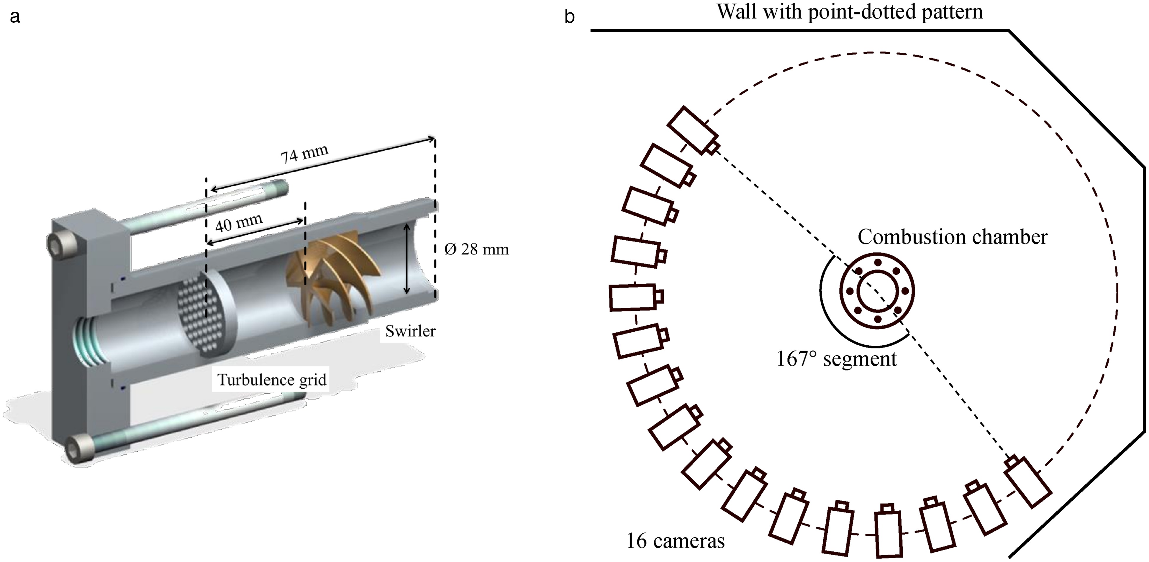
As shown in Figure 2, the combustion chamber consists of eight combustors of which each includes a swirler. The hub and tip geometries are formed by an inner and outer casing creating an annular flow domain. Downstream of this annulus, air exits the test bed as an open jet. More information on the experimental rig can be found in von der Haar et al. (2016) and Hartmann et al. (2016). Immediately downstream of the annular test geometry, BOS measurements were conducted in the jet using 16 cameras. The cameras were mounted equidistantly 11.75 deg apart from each other on a half ring with a diameter of 1.95 m. The cameras face a point-dotted pattern as shown in Figure 2. The camera resolution is 1624 × 140 pixels where a single dot corresponds to 3–4 pixels. 500 pictures were taken with each camera at a sampling rate of 50 Hz. The exposure time equals 150 µs which can accurately capture the low-speed flow at 5 m/s. Each camera picture is divided into square-shaped windows of 32 pixels each. Per the methodology given, a tomographic reconstruction is conducted for each window yielding the density distribution in the jet.
Figure 2.
Schematic depiction of combustion chamber tests. (a) Combustor geometry (adapted from Hartmann 2020). (b) BOS measurement setup.
The combustor was investigated experimentally for its nominal operation as well as three characteristic defects and their superposition. The defects investigated expand upon the work detailed in Hartmann et al. (2018) where a smaller subset of defect cases was presented. The investigated defects can be grouped into three studies: Changing the thermal power of a single burner while keeping the fuel-to-air ratio
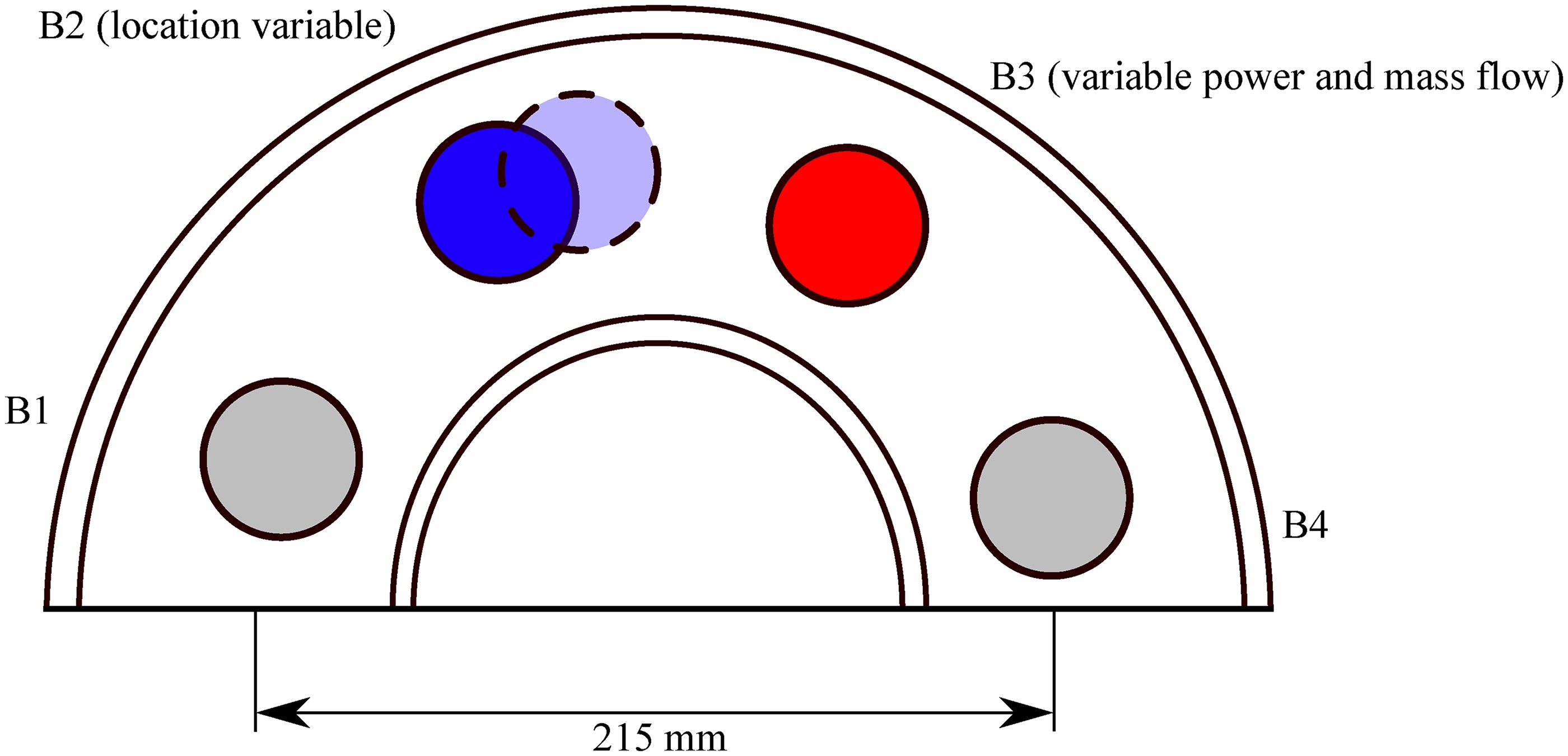
Table 1.
Operating points and simulated defects for the model combustor. Adapted from Hartmann (2020).
For series A, the output power of burner B3 was reduced in eight steps until a full blockage, i.e., simulated failure of the burner, occurred. Keeping the burner power constant in series B caused rich or lean combustion to occur.
Numerical simulation of an aero-engine hot-gas path
In order to extend the experimental SVM analysis to automatic defect detection in an aero-engine exhaust jet, numerical simulations of a hot-gas path components were conducted. The simulated domain consists of a two-stage high-pressure turbine (HPT), a five-stage low-pressure turbine (LPT), exit guide vanes (EGV), and a thrust nozzle as depicted in Figure 4. A detailed description of the numerical setup is given in Hartmann and Seume (2018).
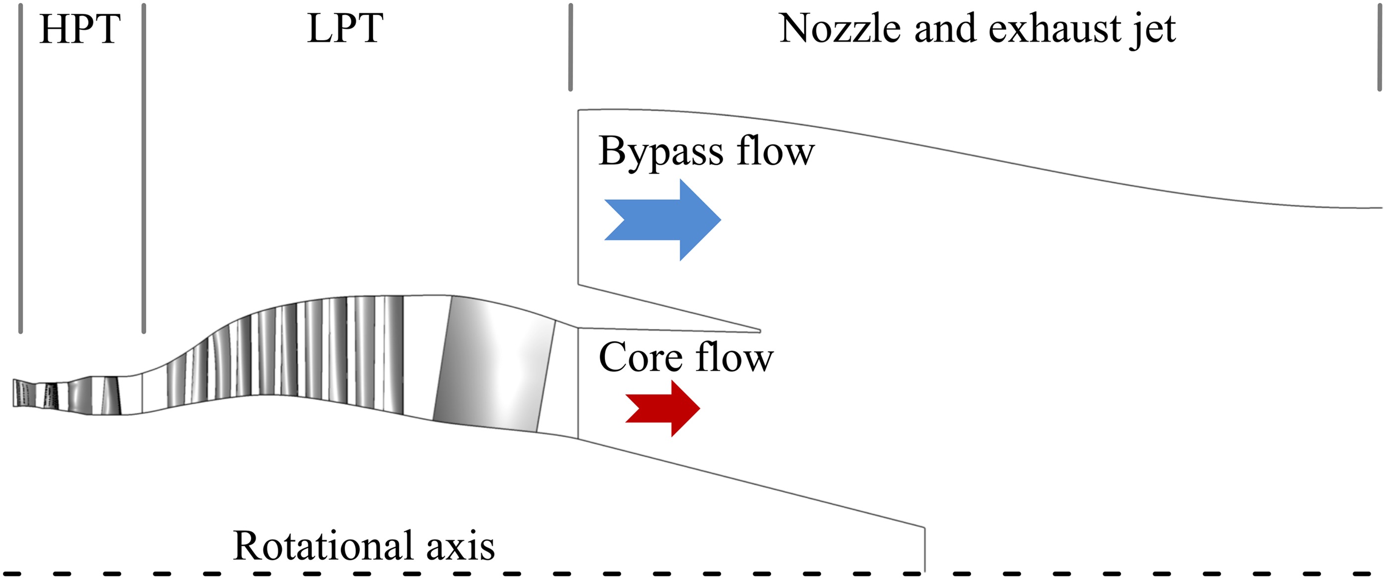
All simulations were performed using the TRACE solver (Franke et al. 2005) , which is developed at the Institute of Propulsion Technology of the German Aerospace Center (DLR). Steady-state simulations were performed using the Wilcox k-ω turbulence model (Wilcox, 1988) for the HPT, LPT and EGV, as well as the Menter SST model (Menter, 1994 implemented in the version provided by Menter et al., 2003) for the thrust nozzle and the exhaust jet. The operating point chosen for these simulations is typical for ground operation, as this represents a potential use-case for BOS measurements in a maintenance scenario. At the HPT inlet, total temperature and total pressure boundary conditions obtained from a combustion chamber simulation are prescribed. In order to preserve the flow disturbances in the exhaust jet, rotor-stator interfaces between HPT and LPT rows are prescribed as direct interfaces, i.e., frozen rotor simulations are conducted. For the inlet boundary condition, a radial total temperature distribution obtained from a combustion chamber simulation is used. The total pressure at the reference point equals 3.18 MPa and is readjusted for subsequent defects to keep LPT power constant. At the outlet, constant atmospherical backpressure is prescribed for all operating points.
Two different defects as well as combinations of both were numerically investigated. The defects, an increased radial gap and a reduction of the film cooling air mass flow within the first HPT stage, are distinctive for wear in the hot-gas path. The tip gap defect was simulated by modifying the computational grid and the cooling mass flow rate by changing the associated boundary conditions. The defect variation amplitude and their combinations are detailed in Tables 2 and 3. Despite this work utilizing numerical simulations, previous studies have shown that these defects can also be measured in a real engine using tomographic BOS (Adamczuk and Seume, 2016).
Table 2.
Variation of relative film cooling mass flow for HPT Vane 1 and Blade 1.
| OP | Vane | Blade |
|---|---|---|
| Ref | 100% | 100% |
| V75% | 75% | 100% |
| V50% | 50% | 100% |
| B75% | 100% | 75% |
| B50% | 100% | 50% |
Table 3.
Variation of tip-gap height of HPT Blades 1 and 2.
| OP | Blade 1 | Blade 2 |
|---|---|---|
| Ref | 1% | 1% |
| C13% C21% | 3% | 1% |
| C11% C23% | 1% | 3% |
| C13% C23% | 3% | 3% |
| C15% C23% | 5% | 3% |
| C13% C25% | 3% | 5% |
| C15% C25% | 5% | 5% |
The thrust of a turbofan aero engine depends on the power of the low-pressure turbine which powers the fan. Since the thrust of the engine must be constant independent of its condition, the power of the LPT was kept constant throughout this study too.
Results and discussion
The described methodology, i.e., Background-Oriented Schlieren (BOS) measurements evaluated using a Support Vector Machine (SVM) algorithm, was applied to the two test cases. The ability of the SVM to automatically identify defects like partly or fully blocked burners is shown using the experimental combustion chamber rig. Finally, it is shown that the SVM can even detect and distinguish combined defects in the high-pressure turbine of an aero engine. The results and discussion presented were taken from Hartmann (2020).
Automatic detection of combustion chamber defects
BOS measurements
The reconstructed density fields obtained from the BOS measurements form the basis for training and validating the defect detection using an SVM. Since the focus of this paper lies on the machine-learning based evaluation, these measurements will only be briefly discussed here. More information on the physical influence of burner defects on the flow field can be found in Hartmann et al. (2016). Figure 5 depicts the reconstructed density field of several operating points (OP) with A1 describing nominal operation. Burner B3, which is altered to model defects, is marked in white.
Figure 5.
Density distribution in the exhaust jet of the model combustor as measured by tomographic BOS (adapted from Hartmann 2020).
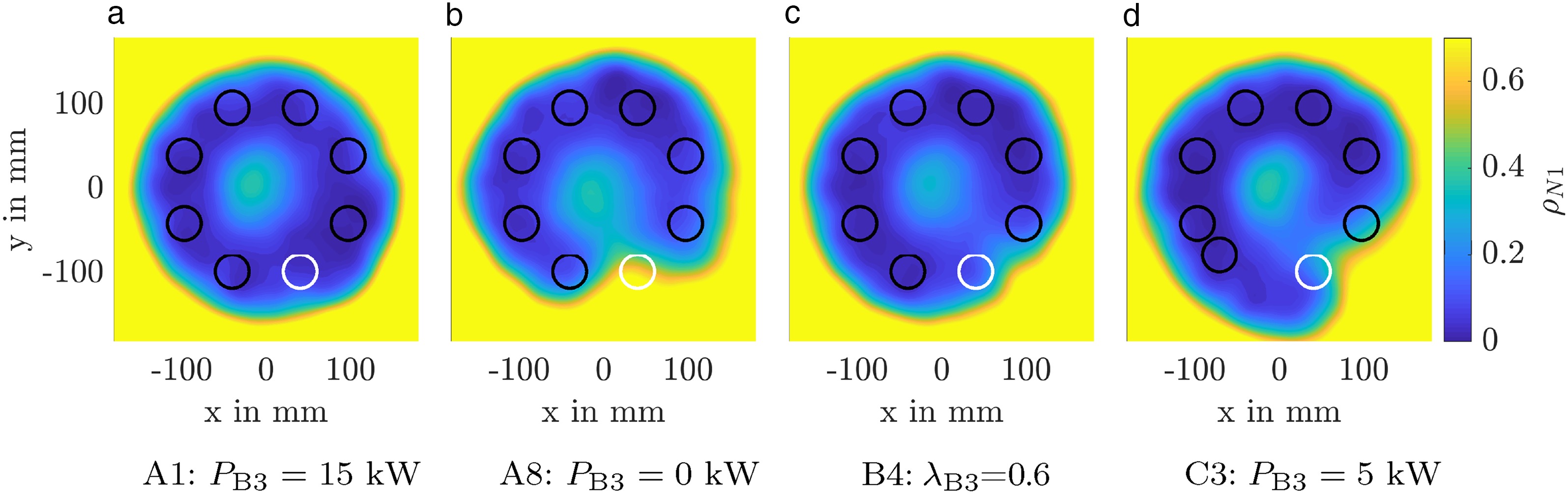
The density is normalised per
to obtain a clear frame of reference and more easily identify defects. For nominal operation (A1), an annular region of homogeneous low-density forms which is bounded by a high-density region outside of the exhaust jet. In the center, another region of higher density can be also identified, which is not as strongly affected by the combustor flow. If the combustor B3 is shut off, the high density outside region expands into the annular section. For lean combustion (B4) the local density increases as well. In OP C3, where burner B2 has been moved in circumferential direction, as is visible in Figure 5d, and power of burner B3 has been reduced, the high-density region extends further inwards compared to OP A8. All operating points deviating from nominal operation, which will be called defect cases in the following, thus show a non-axisymmetric density distribution. Comparing operating points C3 and A8, it is apparent, that several defects occurring at the same time result in a superposed density distribution. While defects are clearly visible in the density distributions, the challenge is now training an SVM to automatically detect these defects.
Training and selection of parameters
The training of the SVM requires separating the data set into a reference class and a defect class. In order to have a critical amount of data for the reference class, this class is defined by the five operating points equal or close to nominal operation (OP A1, A2, A3, B1, and B2), which show only a small influence on the density distribution. The defect class contains the 15 remaining operating points deviating from the reference. For each operating point, 500 pictures per camera were taken for BOS evaluation. From each picture, the density distribution is reconstructed by comparing to the base picture without flow. In order to increase the data base for training and validating the SVM algorithm, 25 random reconstructions were averaged to obtain a new density distribution while maintaining statistical independence. An analysis of the change in the averaged density field revealed that this is possible with only 25 pictures, rather than the 500 of the actual measurement. This finally yields 20 unique measurements - one real measurement and 19 recombinations - per operating point, thus increasing the total data set to 100 reference cases and 300 defect cases. Two thirds of the complete data set is used for calibrating the SVM while the remaining third is used for validation. The challenge lies in defining appropriate non-dimensional parameters to describe the density distributions and their sensitivities with respect to defects. The parameters must be able to identify the characteristic differences between the density distribution of a reference and that of a defect case. For the combustion chamber test case, the aim of training the SVM is only to detect if a defect is present or not. This detection should occur independent of the spatial defect location. For this purpose, integral parameters are defined. Building on the characteristic parameters identified in Hartmann et al. (2016), a total of 11 integral parameters are proposed here.
These parameters are listed in Table 4. In addition to the normalised density distribution introduced above, aerodynamic (entropy, magnitude of the density gradient) and stochastic parameters (mean, standard deviation, skewness, third moment, kurtosis) are specified. As mentioned above, the defect detection should be independent of its circumferential location, which is why the annulus is segmented into eight regions as per the burner number. For each segment, an average
Table 4.
Definition of non-dimensional integral parameters to describe the density distribution and its sensitivity to defects.
With the data set separated into reference and defect classes and appropriate evaluation parameters defined, the next step is training the SVM as described in the methodology section. The entire data set was separated into a data set for training (267 cases) and a data set for validation (133 cases) using the algorithm proposed by Kennard and Stone (1969). The algorithm guarantees that the data set for training and validation represents all classes, i.e., defect and reference classes. The order of the parameters for the SVM was chosen automatically by the Recursive Feature Elimination (RFE) algorithm proposed by Yan and Zhang (2015) and leads to the order given in Table 5. An optimisation of the parameters for the RBF-Kernel helped to find an almost linear hyperplane between the classes with fewer support vectors compared to an automatic choice of parameters.
SVM validation
As shown in Figure 6, with only two integral parameters as per Table 4, 99% of all defect cases and 87.8% of all reference cases are correctly identified. Only 1% of the defective burners were identified inaccurately as belonging to the reference class by the SVM. These mis-predictions represent four measurements of reference case B1 and one measurement of defect case B3. B3 marks a defect case with only minor deviation to nominal operation. Therefore, this point is close to the separating line between the reference and the defect classes in the SVM and the probability of wrong classifications increases. All other cases are correctly classified.
Figure 6.
Influence of the number of parameters on the classification results (validation data set, adapted from Hartmann 2020).
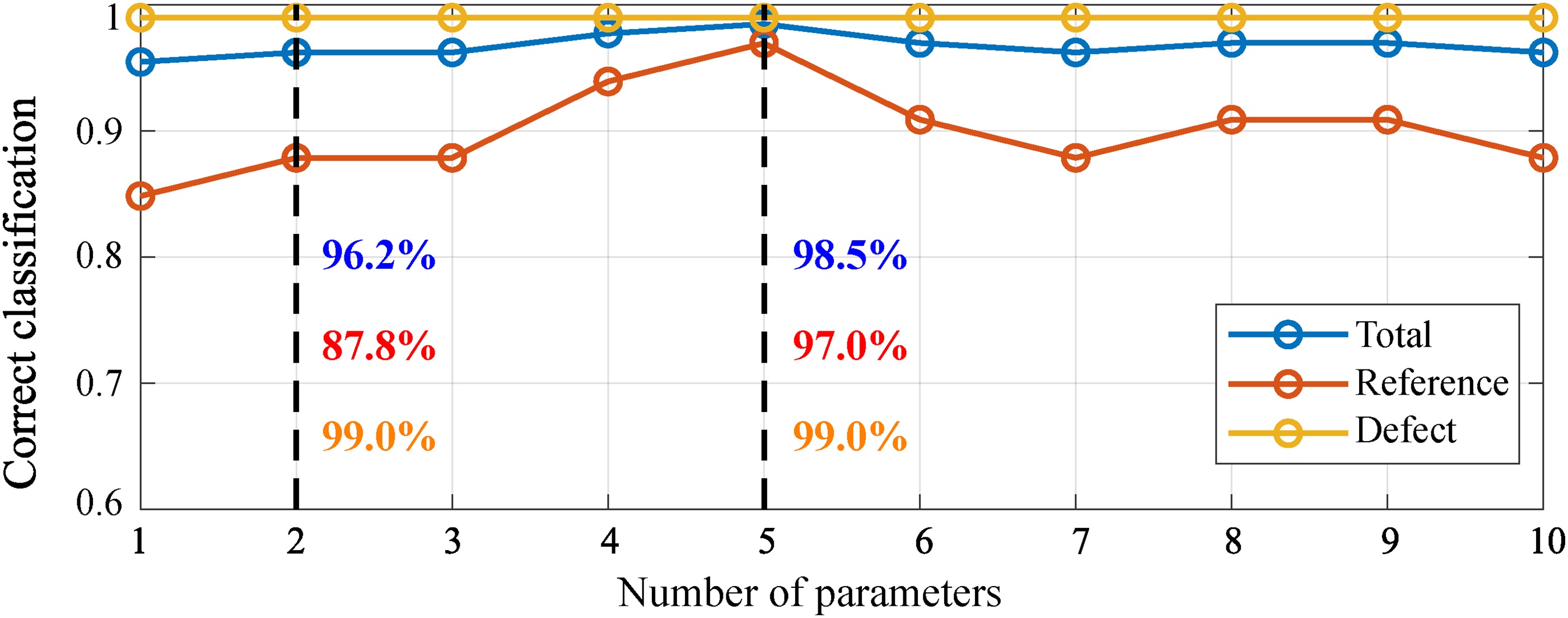
The classification results improve, when the number of parameters is increased and reaches a maximum of 99% for the defective combustors and 98.5% for the reference combustors when five parameters are used. Only one measurement for case B1 and one for case B3 fails when five parameters are used for the SVM evaluation. Possible reasons for the worse classification results with more than five parameters are contradictory dependencies of the parameters (Table 4) on the defects or an over-fitting of the multidimensional hyperplane. Despite the mis-predictions detailed, SVM-based evaluation using the integral parameters proposed, is generally capable of reliably detecting defects in the combustion chamber outlet flow field.
The probability of an accurate prediction can be assessed using a-posteriori probabilities as proposed by Platt (2000). For case B1, this probability equals 79% when 2 parameters are used for the SVM evaluation and 73% when five parameters are used. For case B3, the probability equals 57% for 2 parameters and 83% for five parameters. Cases with a-posteriori probabilities below a certain threshold could be tagged in an industrial application to automatically flag low-confidence classifications for manual evaluation.
Automatic detection of hot-gas path defects in an aero engine
The methodology and parameters derived from the experimental combustion chamber measurements are transferred to an actual aero engine. This test case aims at demonstrating that SVM-based evaluation is not only capable of detecting if a defect is present or not, but also detecting what kind of defect occurred.
BOS measurements
As described above, numerical results are used for synthetic BOS measurements. These yield a data base similar to that obtained from real experiments. Figure 7 depicts the influence of the investigated defects on the circumferentially averaged outlet flow field. Measurement errors represent the noise introduced to model real measurements within a 95% confidence region. Decreasing cooling mass flow causes a reduction in density across the entire span (Figure 7a). Cooling fluid is mixed with the hot gas to a lesser degree, causing a rise in temperature and consequently a drop in density. Increasing the tip gap likewise causes a rise in temperature due to increased losses and thus also a drop in density. Unlike cooling mass flow reduction, however, the density decrease occurs only locally at the casing above radii of 130 mm.
Figure 7.
Influence of defects on circumferentially averaged density (adapted from Hartmann 2020). (a) Absolute density. (b) Normalised density. (c) Normalised local density.
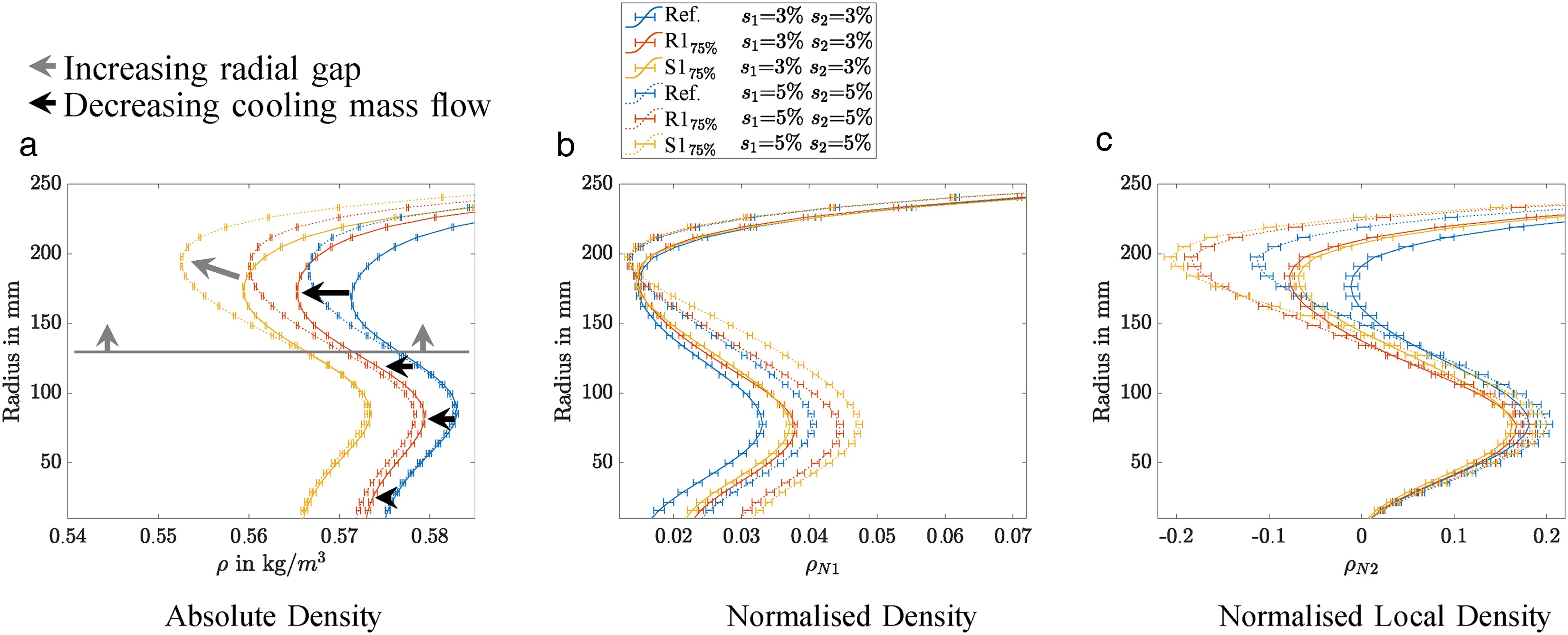
The density obtained is again normalised per Equation 3. A second, local normalisation
is introduced. Both normalisation methods are shown in Figure 7b and c. The local normalisation allows distinguishing between cooling related defects and tip-gap related defects, which is also supported by a subdivision of the engines exhaust jet by its radius R. Therefore,
Training and selection of parameters
Similar to the model combustor, the parameters given in Table 4 are also used to identify defects. A one-versus-all approach is used to perform the multi-class SVM classification. Again, two different sets of training and testing data are defined and two SVM classifiers are trained to detect each defect on their own. The reference class is given by all combinations with a relative cooling mass flow of 100% in vanes and blades, as well as relative tip-gap deviations less than or equal to 3% of the reference gap. This yields 350 reference class cases and 1400 defect cases for the cooling as well as 1000 reference class cases and 750 defect class cases for the tip-gap variation. Again, two-thirds of this data is used for calibrating the SVM while the remaining third is used for validation.
Training and testing data consist of data samples from the reference class and the defect class. They are allocated by using the algorithm proposed by Kennard and Stone (1969). The data set used for training was modified by a Latin-Hypercube Sampling algorithm according to Stein (1987) achieving a more robust hyperplane between the classes. During the training, a false classification of defective engines as reference engines was punished by a weighting factor twice as high as the factor for false classifications of reference engines as defective engines. This procedure is motivated by the fact that false classifications of defective engines as reference engines my cause critical situations during the flight of an airplane with the possibility of human damage.
Again, the order of parameters used by the SVM was optimised by the RFE algorithm as proposed by Yan and Zhang (2015) and is listed in Table 6 for the cooling defect and in Table 7 for the tip-gap defect.
SVM validation
Figure 8a shows the classification results for cooling defects as a function of the number of parameters. Using one parameter only, the SVM correctly identifies 99.9% of all cooling defects and 99.2% of all tip gap defects.
Figure 8.
Influence of the number of parameters on the classification results for both defects (validation data set, adapted from Hartmann 2020). (a) Cooling defects. (b) Tip-gap defects.
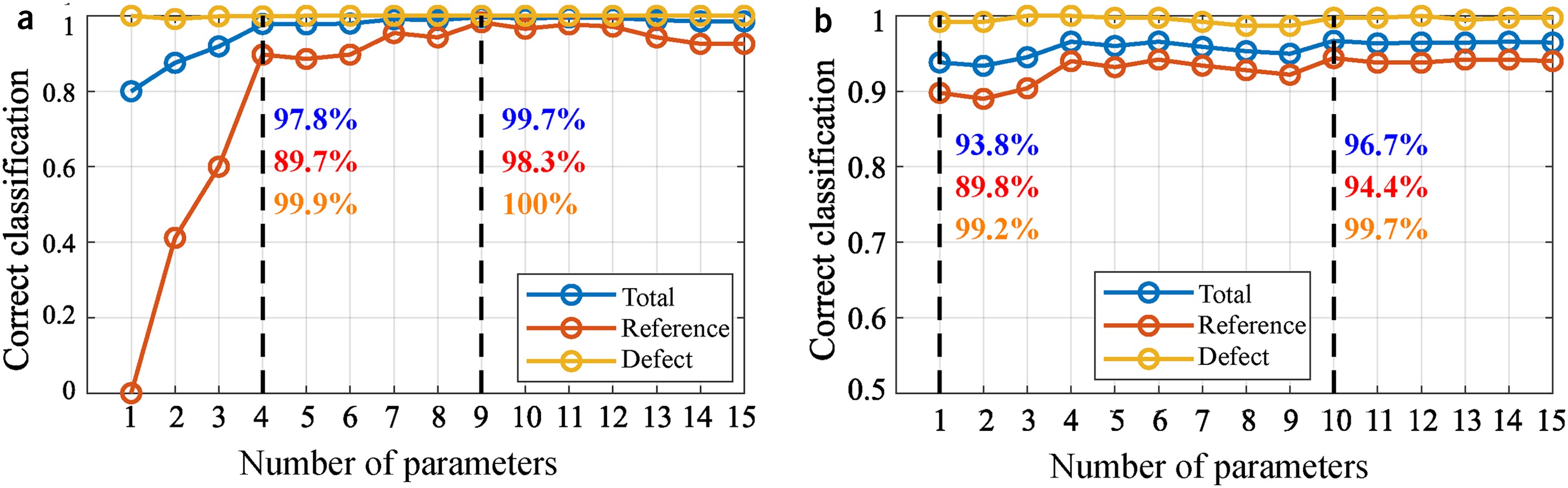
For the cooling defect, the mean density
For the tip gap defect, even one parameter is sufficient to identify 99.2% of all defects and 89.8% of all reference engines correctly, improving to 99.7% and 94.4%, respectively, when 10 parameters are used. In this case, only engines with the largest possible tip gap defect in the first rotor or the smallest possible tip gap defect in both rotors were classified wrongly.
The successful classification of both defects shows that the choice of parameters was sufficient to allow for an automatic separation of defect and reference cases based on the density distribution in the exhaust jet of an engine. Although it is not shown here, the wrong classifications for the cooling mass flow can be compensated since the classification for the tip gap defect correctly identifies these engines as defective. In total, 100% of the defective engines in the data set for testing have been identified.
Application of single-class SVM to jet engines
Finally, the potential of single-class SVM algorithms is investigated. These are particularly suitable for the detection of anomalies, i.e., deviations from a reference class. Unlike two-class SVM, single-class SVM cannot distinguish between different defects. However, this turns into an advantage because no labelled data set with known defects is required for training. This is particularly interesting for industrial applications, where predictive maintenance is conducted and the experience (or data) regarding the effect of defects on nominal flow is insufficient.
In this study, the data set was divided into a reference class and a defect class identical to the two-class algorithm detailed above. Half of the reference data were used for training. The second half and all defect cases were used for validation.
The classification results depicted in Figure 9 show that 100% of all reference engines and 91.4% of all defect engines are classified correctly when five parameters from Table 4 are used. This improves to 100% and 97.7% respectively, when 11 parameters are used. Only engines with 25% reduction of cooling mass flow or an increased tip gap in one of the stages are classified inaccurately. These cases mark defects with comparatively small deviations to the reference.
Figure 9.
Influence of the number of parameters on the classification results for single-class SVM (adapted from Hartmann 2020).

Limitations and practical applications
The SVM-based analysis presented is based on experimental data of a combustion chamber and numerical RANS-simulations of the hot-gas path of an aero-engine. Since these steady-state RANS calculations under-predict the mixing process in the turbine, the low-density regions representing potential defects are likely to be mixed out to a higher degree in a real engine. Nevertheless, preliminary BOS measurements of an aero-engine were similarly capable of capturing such defects, albeit they have not yet been applied to SVM training. Turbine power was kept constant as a boundary condition for all defects introduced, but in a real engine such defects will also cause the operating point to deviate – a failing burner will be compensated by higher power of the other burners to maintain turbine power – thus introducing another effect. This change in operating point does, however, primarily cause a shift in the mean state, meaning that the density normalisation presented will remain independent of such effects. Indeed, if the power of the remaining burners increases to compensate a failure, defects will likely become even more apparent in the density signature.
Another limitation of the methodology presented is that the SVM has so far only been trained to detect both individual and combined defects. While this allows the identification of defective components, another important aspect for industrial applications is to additionally assess the criticality of a defect. This is generally possible within this framework by e.g., using the magnitude of the low-density region, but cannot yet be addressed.
BOS measurements are optical non-contact measurements which can be rapidly conducted without opening the engine. The approach presented is thus suitable for on-ground engine maintenance, as the measurement system can be designed in a highly portable way, only requiring cameras to be mounted on a movable frame. Such measurements could thus be conducted during routine engine tests – theoretically even on-wing. This would allow for automatically detecting defects in the engine and derive maintenance procedures for the affected components. With the a-posteriori probability evaluation presented, it is also possible to flag low-confidence measurements for manual assessment.
As including a permanent BOS-measurement instrumentation is unrealistic, the approach presented cannot by applied to online monitoring. An SVM could potentially be trained using regular engine instrumentation, but the much lower resolution will most likely not allow for a similar detection, particularly that of combined effects.
Conclusions
In this work, the suitability of machine-learning based methods for automated defect detection was evaluated using measurements downstream of a combustion-chamber rig and numerical simulations of the hot-gas path of an aero engine. Support Vector Machine (SVM) algorithms were chosen for this automated detection because of their advantages regarding incomplete data sets. The measurements used for training and evaluating an automated defect detection SVM algorithm are obtained using the tomographic background-oriented schlieren (BOS) method.
Algebraic BOS reconstruction algorithms are used to reconstruct the density distribution in the exhaust jets. In a model test of an annular combustion chamber, introduced defects leave distinct signatures in the density distribution which can be captured using BOS. Synthetic BOS measurements obtained from numerical simulations of an aero engine hot-gas path similarly capture defects such as cooling mass flow variation and radial gap changes. The BOS data are subdivided into two classes: a reference and a defect class.
Using this data set, a parameter set including aerodynamic and stochastic parameters suitable for characterising the density distribution was obtained. These parameters were used for training and validating the SVM. If a sufficient number of parameters is chosen, SVM is able to detect whether defects are present in the combustion chamber. For a selection of five parameters, only one misclassification for an operating point deviating only slightly from the reference occurred. Using an a-posteriori probability analysis, an uncertainty can be assigned to each SVM classification result.
The identification parameters and evaluation methodology was then transferred to numerical aero-engine simulations. A suitable selection of parameters is not only capable of detecting the occurrence of defects but also capable of distinguishing between the individual defects if a multi-class SVM is used. For the parameters chosen, less than 4% of all 1750 cases were wrongly classified. Using a single-class SVM, which is no longer capable of distinguishing between individual defect types, increases the number of correctly predicting defects to almost 98%. The results also show the importance of choosing a suitable parameter space for this SVM evaluation.
It can be concluded that automated defect detection using SVM algorithms to evaluate BOS measurements is capable of detecting and classifying defects in the exhaust jet. The a-posteriori probability evaluation can be used to flag remaining misclassifications as low-confidence for later manual evaluation. In an industrial application, where BOS measurements are comparatively simple to conduct, SVM would thus be capable of a reliable and robust defect detection.
Future investigations will comprise BOS measurements of a real aero-engine, thus aiming to validate the numerical results presented and also assessing combined effects such as a resulting deviation in the operating point. These tests will also expand the available data base for a criticality assessment tremendously in addition to detecting the presence of defects.