Introduction

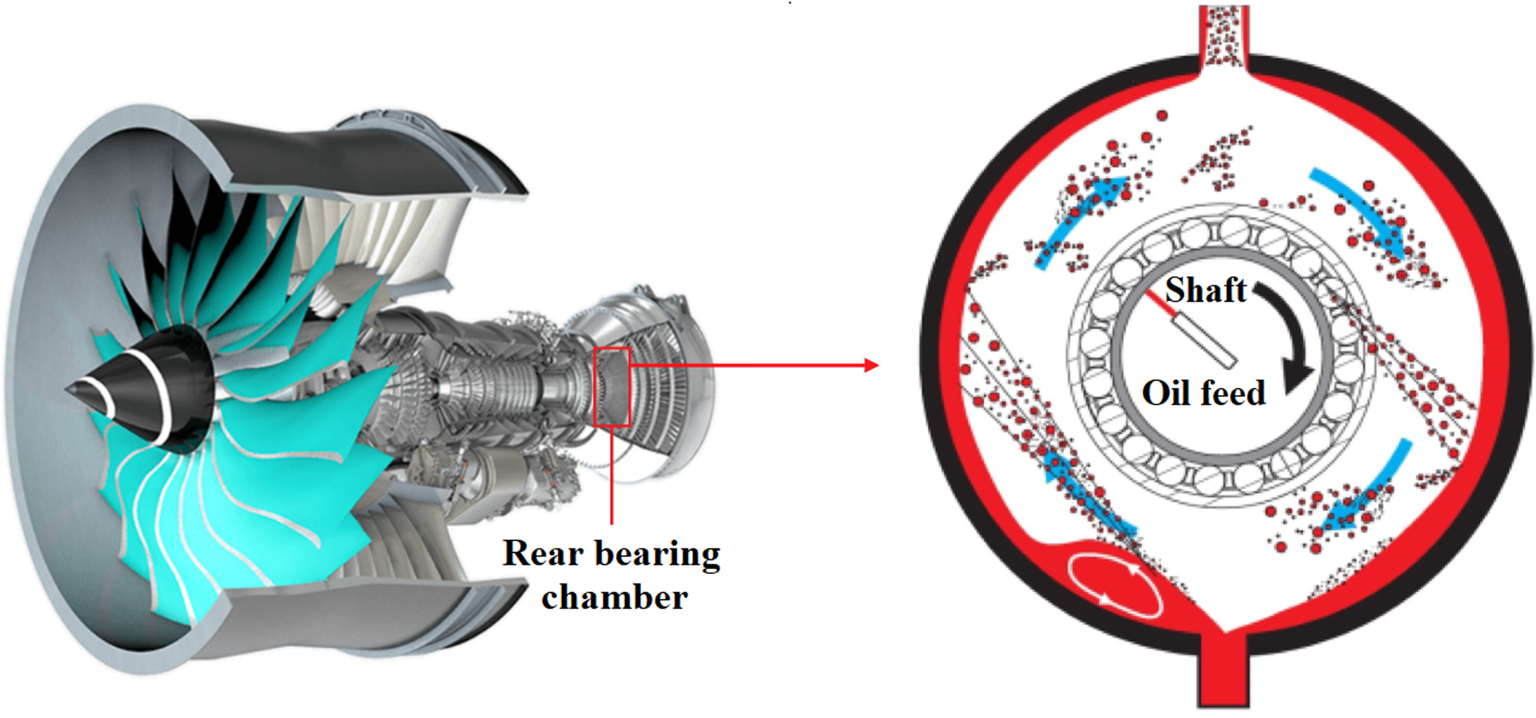
The prediction of the oil film thickness distribution plays an important role when it comes to improving and optimising the design of aero-engine bearing chambers. A schematic of the cross-section of a bearing chamber is shown in Figure 1.

Figure 1.

Rolls-Royce Ultrafan aero-engine and cross-section schematic of a bearing chamber (Rolls-Royce Plc, 2016).

Whilst the design of bearing chambers is mainly based on experiments, research focuses on finding adequate approaches to model two-phase air/oil shearing flows with Computational Fluid Dynamics (Bristot et al., 2016). However, modelling turbulent two-phase shearing flows with a sharp interface in an industrial context can be challenging due to the combination of a multiphase flow problem and the effects of high speed regimes. On the one hand, accurate results using CFD might be obtained in exchange for a high computational cost (Adeniyi et al., 2014), which is not practicable in an industrial context. On the other hand, averaged simulations would limit computational costs (RANS), although they struggle to treat the high velocity gradients in the interfacial region (Frederix et al., 2018), causing an overestimation of the levels of turbulence at the interface, corrupting the velocity and energy profiles and causing inaccuracies in the prediction of the flow. Egorov et al. (2004) proposed a correction for the RANS k−ω model’s transport equation of the specific turbulence dissipation rate ω by adding a source term Sω to reproduce a wall-like treatment at the interface between the liquid and the gaseous phase. This source term is controlled by a turbulence damping parameter B, which choice depends on the flow conditions and the expected solution. One could write this corrected ω transport equation in the standard unsteady RANS k−ω model (Wilcox, 1998) as follows:

With ρ the flow density, ui the velocity, k the turbulent kinetic energy, μ the dynamic viscosity, Pω the production term,γ and β coefficients of 0.55 and 0.075 respectively. The correction source term for the ω transport equation Sω is written as follows:

The subscript i denotes the phase (either gaseous or liquid), A is the interfacial area density used as a switch to ensure that the source term is only applied in the interfacial region, Δx is the representative cell size across the interface and ν is the kinematic viscosity. The application of the Egorov’s correction results in a better treatment of the interfacial turbulence dissipation and provides more accurate solutions. While Egorov et al. (2004) recommended a value of 100 for B, Lo and Tomasello (2010) used a value of 2,500 to match experimental measurements. Bristot (2018) demonstrated that the choice of this turbulence damping parameter strongly influences the interface prediction in the context of bearing chambers’ two-phase flow. For example, the researcher compared results using the RANS k−ω Shear Stress Transport model (SST) with Egorov’s correction for two values of B (10 and 100) at the same bearing chamber flow regime of 15,000 rpm. It was indeed found out that predicting physics is very sensitive to the choice of B as shown in Figure 2. The correction source term Sω is strongly mesh dependent (Frederix et al., 2018; Fan and Anglart, 2019) and there is no guidelines on setting B. Egorov et al. (2004) were pioneers in assessing and addressing the standard model’s weakness to evaluate the interfacial turbulence in stratified flows with high gradient of velocities across the interface. More recent research have has focused on improving the Egorov’s method. Fan and Anglart (2019) proposed a novel approach with more physics and made the Egorov’s method mesh independent with an asymmetric treatment of the two phases, leading to more physical predictions of the flow turbulent kinetic energy and velocity especially in the interfacial region. Frederix et al. (2018) extended Egorov’s method to the k-ε model for the two-fluid formulation (Euler-Euler approach) giving more consistent results for a various of computational grids than the original Egorov’s method. Hashmi et al. (2010) developed an ‘enhanced VOF model’ with a refined interface treatment and obtained promising results when applying their method on a few stratified flow cases using the RANS k-ε model.

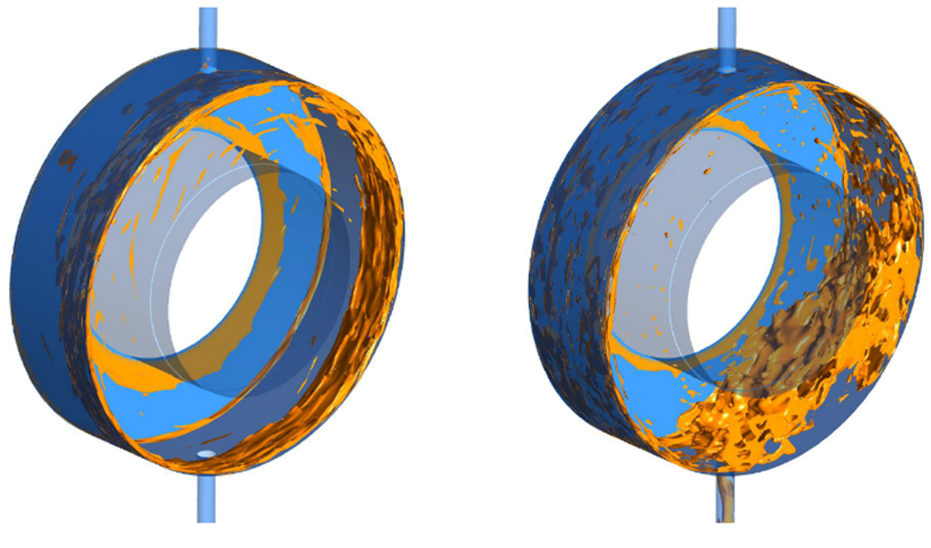
Figure 2.

Oil film thickness distribution influenced by the turbulence damping parameter B=100 (left) and B=10 (right) at the same flow regime (Bristot, 2018).

The use of machine learning (ML) in computational fluid dynamics has become more and more common as the field of data science is gaining in popularity in industry. One of the best current features of ML in CFD is the improvement of existing low order turbulence models such as RANS models, thanks to high fidelity simulations such as DNS or LES data-driven ML models.

One can use ML to compute the source terms in the transport equations of RANS turbulence models. For example, Tracey (2015) used ML in order to reproduce the Spalart-Allmaras RANS model. They modified the solver in a way that used the output of the ML model instead of the standard Spalart-Allmaras model’s source term. The ML model was trained with a flat plate simulation dataset and used for the simulation of the flow around an airfoil. When looking at the friction coefficient, the author found very good agreement between the ML and the Spalart-Allmaras model. Despite the ML model giving promising results, the author warned that the differences found between prediction and true data could be explained by the fact that the ML algorithm was trained only with converged flow solutions. Singh (2018) used multiple sources of data for ML model training such as DNS, LES and experiments. Here, ML methods were used to improve the Wilcox’s RANS k−ω model for adverse pressure gradient flows such as flows over a bump. The author focussed on adding a correction function in the k−ω equations applied to the production term. This correction was used to change the net balance of the source terms improving the standard model. Results demonstrated a great improvement of the solution.

This paper aims to address the problems related to the Egorov’s correction by generating a mesh and coefficient independent correction for the ω transport equation from high fidelity simulation data and more specifically by training a a ML model to predict a correction source term on various cases and flow conditions. It is embedded as a process within the open source CFD code OpenFOAM, in order to improve the standard Wilcox’s RANS k−ω model. The objectives of this paper are to first generate training data using quasi-DNS (qDNS) using OpenFOAM, then implement an appropriate ML model capable of predicting proper corrections for the simulated case. Finally to include the implemented ML model within OpenFOAM to provide a correction for the standard RANS k−ω model.

Methodology

The methodology for the current research can be decomposed into three main tasks. The first is the creation of high fidelity datasets for the training of the ML model. Quasi-DNS simulations were carried out in periodic horizontal channels with a liquid phase at the base (water) and a gaseous phase on the top (air). One could assimilate the flow present in a periodic horizontal channel to the flow located on the external wall of a small portion of a bearing chamber with an oil film driven by air shear. Different interface heights and phase velocities were employed to diversify the training dataset. A proof of concept was carried out using qDNS simulations based on experiments (Fabre et al., 1987), which involve air shear over deep water. Then, a second study was performed using a ML model trained with qDNS data on flow conditions closer to the type of flow that one finds in bearing chambers (i.e., shallow water or thin films). The second task of the methodology is the implementation of the ML model, where the choice of the different input features is important and must be performed by considering possible physical links with the output. The number of inputs, layers and the type of neural network used must also be considered in the implementation of the ML model. The implementation of the model was performed within the Python API of the well-known PyTorch open source ML library. The final task of the methodology is the embedding of the ML model within OpenFOAM for unsteady RANS k−ω simulations in a way that it can be reused or easily adapted in future versions of the code.

Generation of the high-fidelity simulation training dataset

The Volume of Fluid method

The Volume of Fluid (VOF) method was used for the purpose of all simulations mentioned in this paper using the solver interFoam available in OpenFOAM. The VOF method describes the flow such that all phases share the same velocity and pressure fields (Hirt and Nichols 1981). The phase volume fraction αi describes how the phases are distributed in the domain. In the case of a two-phase flow problem, where αi=α1 or αi=α2, one can write α1=1−α2. Thus αi becomes a variable quantity of the discretised domain and is advected by the local velocity as:

(3)

∂αi∂t+u⋅∇αi=0

One can then describe flow scalar fields such as the density, kinematic and dynamic viscosity of a two-phase flow as:

(4)

ϕ=α1ϕ1+(1−α2)ϕ2

where ϕ refers to the given scalar field and indices 1 and 2 refer to the primary and secondary phase respectively. The surface tension between the two phases of the problem can be introduced into the Navier-Stokes equations by adding a resulting interaction force F=σ∇⋅n∇αi with n the unit vector normal to the interface, i.e., for incompressible flows:

(5)

ρ[∂ui∂t+∇⋅(ui×ui)]=ρg−∇p+μΔui+F

The VOF method is widely employed in CFD to model multiphase flows and performs well in the case of strong instabilities in free surface problems provided that the mesh is refined enough in the interfacial region (Faghri and Zhang, 2006). In the context of a shearing two-phase flow, it can be challenging to preserve a sharp interface. The interFoam solver comes with a sharpening method of the interface that was implemented by Wardle and Weller (2013). In this method, a compression term is added to the transport equation of αi (Equation 3) as:

(6)

∂αi∂t+u⋅∇αi+∇⋅ucompαi(1−αi)=0

In which ucomp is a compression velocity applied only in the region of the interface and applied normally to it. It is enabled by a compression coefficient Cα:

(7)

ucomp=min{Cα||u||;max||u||}∇α||∇α||=0

All the simulations mentioned in this paper were carried out using a surface tension σ=0.07 and compression coefficient Cα=2.0.

Discretisation schemes and solution methods for qDNS

The VOF solver interFoam was employed with the second order Crank-Nicolson time scheme with a coefficient of 0.9, the second order total variation diminishing (TVD) “van Leer” scheme van Leer (1979) to discretise the divergence terms in the transport equations of αi and second order linear schemes for the other divergence terms. The pressure-velocity coupling is managed by the PIMPLE algorithm. Pressure was solved using the Preconditioned Conjugate Gradient (PCG) method, whilst the phase volume fraction, velocity and kinetic energy were solved using the Gauss-Seidel method.

Formulation of the correction source term

In order to obtain the correction source term Sω for the budget of the transport of the specific turbulence dissipation rate of the standard RANS k−ω model, each term of the ω equation was calculated by qDNS in OpenFOAM using coded functions objects for example Equation (1) can be rewritten as follows:

(8)

Sω=Sadv−Sprod+Sdes−Sdiff

With:

• Sadv=∂ρuiω∂xi: the advection term

• Sprod=γωkPω: the production term

• Sdes=βω2: the destruction term

• Sdiff=∂∂xi[(μ+ρk2ω)∂ω∂xi]: the diffusion term

As all fields are time-averaged during the simulation, the local time derivative term is zero. The specific turbulence dissipation rate is defined as ω=ε/(kβ∗) with ε the turbulent dissipation and β∗ a model constant taken at 0.09. The quantities ui, ε, k and ω are averaged as the simulation progresses within OpenFOAM once the flow is fully developed. This is achieved using the following definition of ε within the VOF solver (Hinze, 1975):

(9)

ε=12ν(∂ui′∂xj+∂uj′∂xi)2¯

where ui′ is the fluctuation velocity such as ui=ui¯+ui′. It should be noted that steady RANS simulations would not fully converge even though the flow exhibited weak unsteadiness and a unsteady RANS (URANS) methodology was adopted. The correction term calculated using qDNS includes contributions from all length scales. As part of future work and for higher Reynolds numbers the removal of deterministic URANS scales will be examined for example using FFT/IFT (see Lav et al., 2019). In the present work the impact is thought to be small and as will be seen the corrected RANS yields lower TKE values compared to qDNS.

Domain geometry, flow characteristics and case presentation

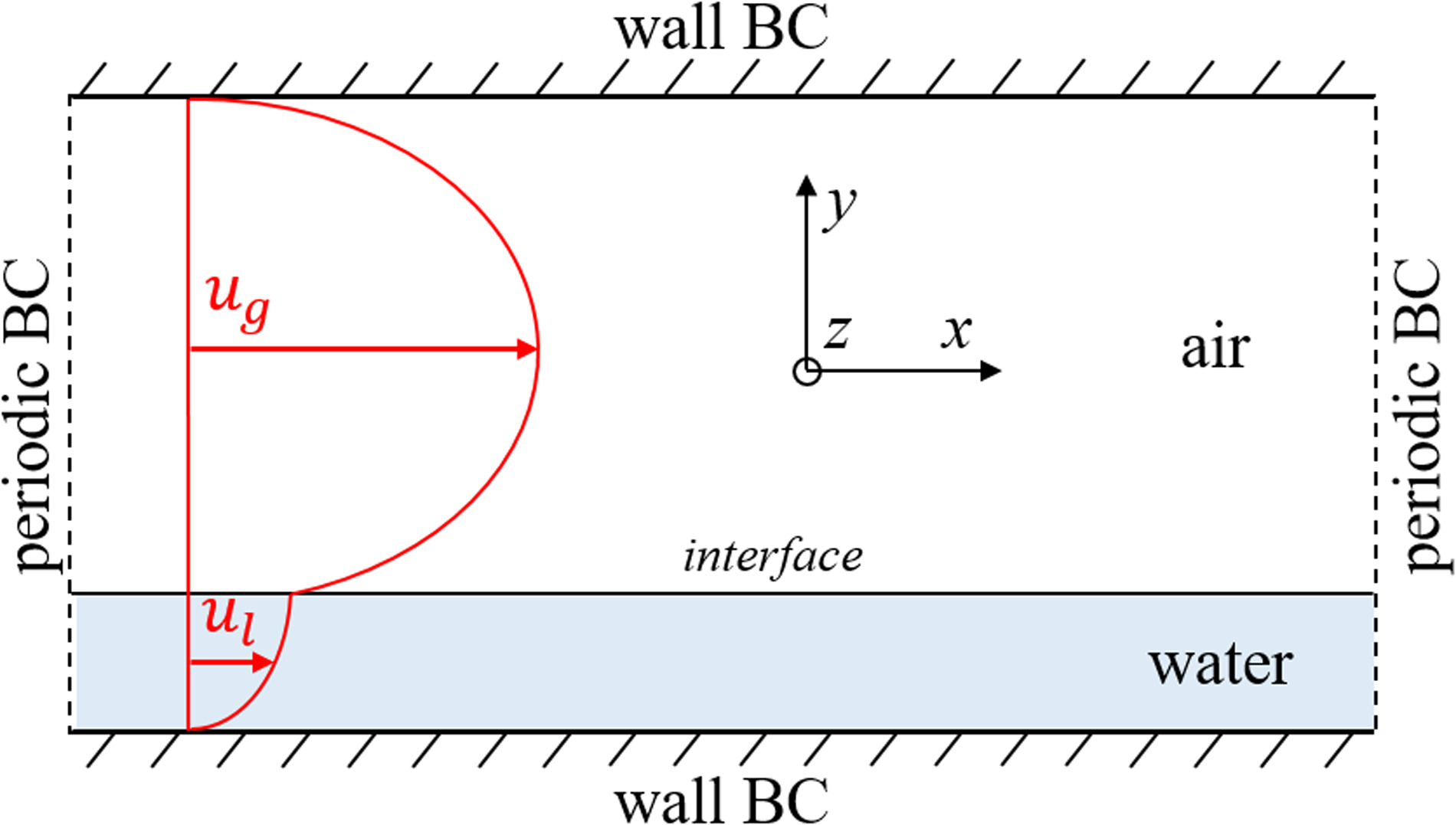
As previously mentioned, two flow configurations were tested. The first one is based on reference experiments (Fabre et al., 1987) and was designed to establish a proof of concept and validate the qDNS methodology. The second configuration is based on a shallow water air-shear driven flow configuration that is more representative of bearing chamber flows containing thin wavy films. These two configurations are referred to as “configuration 1” and “configuration 2” respectively. In both configurations, the liquid and the gaseous phase are co-current and the gaseous phase has a higher velocity than the liquid phase. The liquid phase is water and located at the base of the channel. The gaseous phase on top is air. No-slip boundary conditions are used for the top and bottom walls whilst periodic boundary conditions were used in the flow direction (x) and in the horizontal cross-flow direction (z). Figure 3 gives an overview of the domain and flow setup for both configurations. Both phases are driven toward the streamwise direction using velocity sources added to the velocity transport equations and applied to each phase.

Figure 3.

2D schematic overview of the computational domain.

Configuration 1

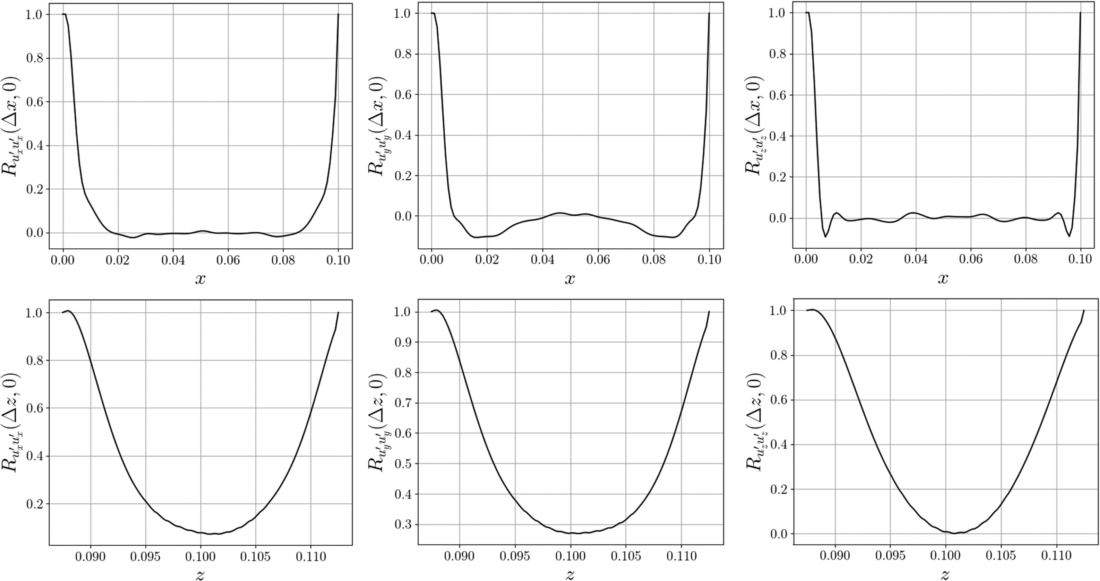
In the reference experiments, the channel is 12 m long, 0.1 m high and 0.2 m wide. The liquid bulk velocity is 0.45 m/s and the gaseous bulk velocity is 4.2 m/s. The computational domain was made periodic for computational cost and a periodic length of 0.2 m in the x direction and 0.025 m in the z direction was used. To examine the extent of the periodic dimensions an autocorrelation study of the flow was performed. The autocorrelation function was used to determine the minimum periodic length; if the periodic length is too small then large turbulent structures can overlap and lead to unphysical results. If the autocorrelation function of the fluctuation velocity drops to zero at a distance half of the periodic length, them this length is sufficient to prevent unphysical results (Fröhlich et al., 2005). The autocorrelation of a quantity is a function of the time lag Δt and space lag Δx where xi=x in the flow direction and xi=z in the cross-flow direction. The autocorrelation of the fluctuation velocity is calculated as follows:

(10)

Rxixi(Δxi,Δt)=uxi′(xi,t)uxj′(xi+Δxi,t+Δt)¯uxi′2(xi,t)¯uxi′2(xi+Δxi,t+Δt)¯

Rxixi is bounded by −1 and 1. A value of 1 indicates that the flow is perfectly correlated and a value of 0 indicates no correlation of the flow. Figure 4 shows the spatial autocorrelation of the axial fluctuation velocity which is the quantity of interest, Rxx(Δx,0), averaged over a period of 10 seconds. We can deduct from the spatial autocorrelation plots that the periodic length is sufficient in the flow direction as Rxx drops to 0 before the half of the length.

Figure 4.

Autocorrelation of the axial fluctuation velocity of the gas in the flow direction (left), cross-flow direction (right) and isosurfaces of instantaneous Q-criterion and contours of instantaneous vorticity magnitude from qDNS based on Fabre et al. (1987) experiments (centre) in configuration 1.

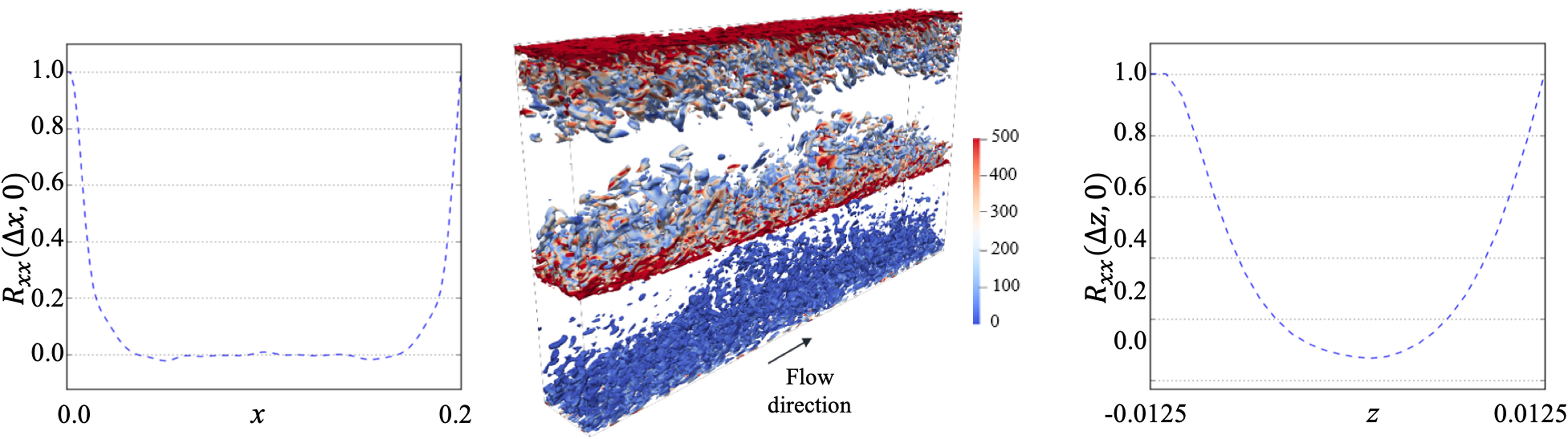
The autocorrelation in the cross-stream direction also reaches a value of zero halfway through the width of the channel and indicates a sufficient decorrelation of the flow in the cross-stream direction. The interface was set at 0.038 m from the base of the channel which gives a liquid layer thickness of 38% of the total height of the channel. A 3D representation of the flow with instantaneous Q-criterion isosurfaces and coloured with vorticity magnitude contours is shown in Figure 4. Additionally, the autocorrelations of all the fluctuation velocity components in both x and z directions are shown in Figure 7, Appendix A.

Configuration 2

In configuration 2, the domain is a periodic channel with similar boundary conditions to configuration 1. The periodic length of the channel in configuration 2 is 0.04 m in the x direction and 0.08 m in the z direction. The channel height is 0.026 m with no-slip boundary conditions at the top and bottom walls. The two-phase flow can be considered as a shallow-water flow.

A range of qDNS cases were carried out in order to produce a diversified dataset for the training of the machine learning model. In those cases, different interface height and bulk velocities for each phase were used. In addition to the training dataset cases, three additional test cases were performed using qDNS for different regimes and interface heights, cfg2-1, cfg2-2 and cfg2-3. The results from these three cases were used as reference for comparison with the corresponding RANS simulations using the RANS k−ω model coupled with the trained ML model. Results were also compared with the standard RANS k−ω model without correction. The bulk velocity Ub and Reynolds number Re of each phase, the mean interface height h¯, the kinematic viscosity ν and the density ρ of each phase are presented in Table 1 for the three test cases.

Table 1.

Flow properties for the configuration 2 test cases.

Property	cfg2-1	cfg2-2	cfg2-3
Ub,g (m/s)	5.20	4.20	5.20
Ub,l (m/s)	7.72×10−3	1.93×10−2	1.93×10−2
Reg	8.2×103	6.3×103	8.0×103
Rel	1.8×101	6.6×101	6.0×101
h¯ (m)	2.33×10−3	3.44×10−3	3.05×10−3
ρg (kg/m3)	1.0	1.0	1.0
ρl (kg/m3)	1.0×103	1.0×103	1.0×103
νg (m2/s)	1.5×10−5	1.5×10−5	1.5×10−5
νl (m2/s)	1.0×10−6	1.0×10−6	1.0×10−6

Discretisation of the computation domain

In qDNS, the grid cell size Δy must be sufficiently small to capture the smallest scales of the turbulence as they are not modelled by a subgrid model, hence a comparison to the Kolmogorov scale η can be done. One Kolmogorov number for each phase is calculated using η=(ν3/ε)1/4 where ε can be estimated as ε∼Ub3/Li in which Ub is bulk velocity of the phase and Li the characteristic length scale of the flow. Hence we obtain the following estimation of the Kolmogorov scale:

(11)

η=(ν3LiUb3)1/4

For the studied stratified flow, the characteristic length scale of each phase is its height h in the channel. The role of the smallest turbulent scales is to convert the TKE into internal energy. When slightly under resolved mesh is used, the role of those smallest scales can still be completed by the remaining resolved scales. For under resolved mesh (Δy>20η), numerical instabilities are more likely to happen and lead to unphysical results. Typically resolved LES or quasi-DNS uses a resolution 2 to 5 times coarser than the Kolmogorov scale (Tiselj et al., 2019). In the liquid phase, Δy was taken at approximately η/12 at the walls and η/8 at the interface, while in the gaseous phase Δy was η at the top wall and 2η at the interface. In terms of wall units, Δy+=0.3, Δx+=8 and Δz+=6.

Results and discussion

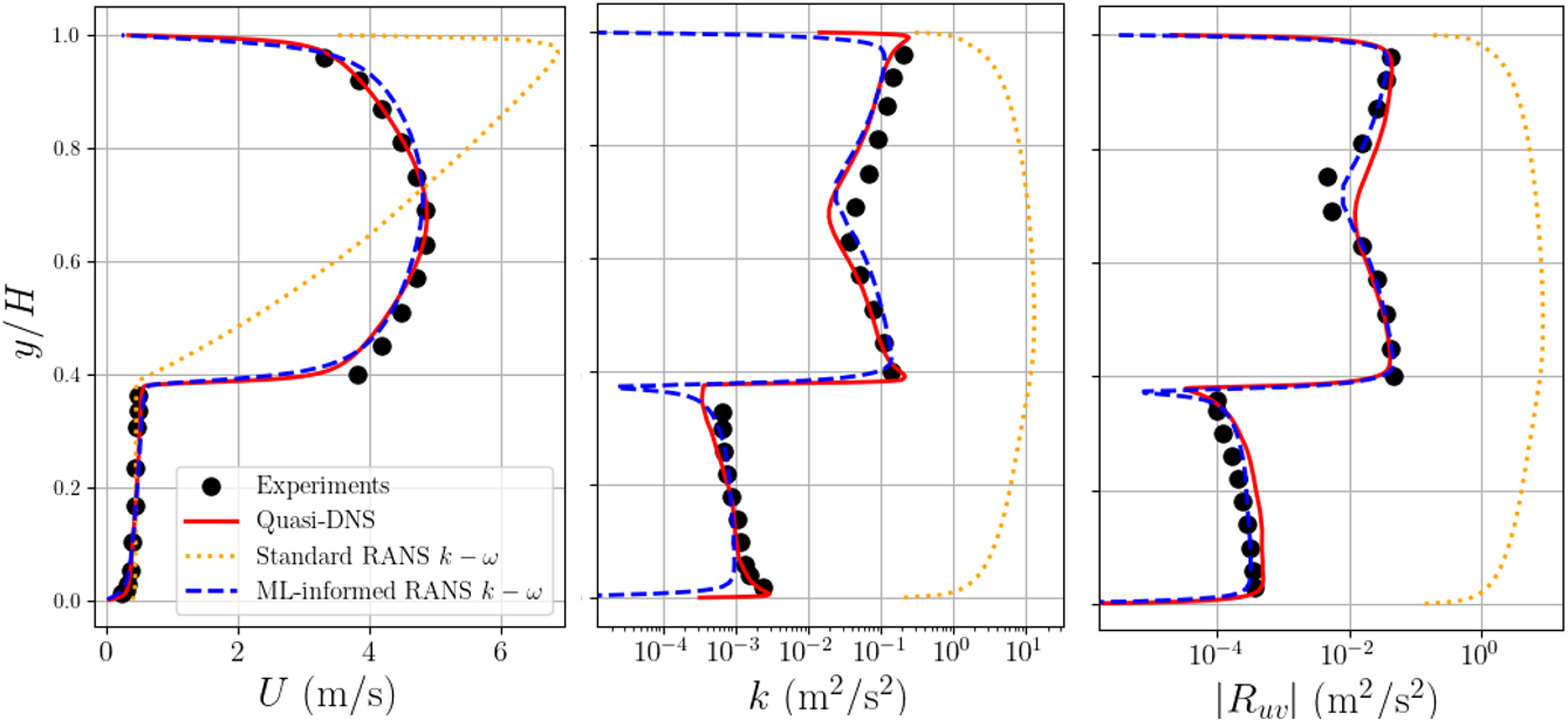
As previously mentioned, in configuration 1 the ML model was trained using a single qDNS dataset based on the Fabre et al. (1987) experiments as described in the methodology section. The RANS simulation was realised using the same flow conditions and coupled with this ML model as a proof of concept. The numerical results obtained from the qDNS and RANS using both the standard Wilcox’s and the ML-informed k−ω model were compared with the aforementioned experiments using three quantities namely the mean axial velocity Ux, the turbulent kinetic energy k and the absolute value of the cross component (in the x, y plane) of the Reynolds stress |Ruv|. Results of the comparison for configuration 1 are shown in Figure 5. The TKE and stress were plotted using a logarithmic scale in order to better evaluate the discrepancies between the results. It is shown that the qDNS results agree very well with the experiments for all quantities and in both phases. Regarding the RANS simulations, it is obvious that the standard Wilcox’s k−ω model performs very poorly. One can observe a shift towards the upper part of the channel of the mean velocity that is directly caused by the uncorrected overestimation of the interfacial turbulence by the standard model. For the TKE and stress profiles, the standard model does not pick up the interface at all (no discontinuity or variation) resulting in values very far from the qDNS and experiments. Finally the ML-informed RANS performs very well with results close to the qDNS and experiments for all three measured quantities. These results illustrate that an appropriate correction of the budget of the transport of the specific turbulence dissipation rate in the RANS k−ω model can provide very good results.

Figure 5.

Comparison between qDNS, standard RANS k−ω, ML-informed RANS k−ω and Fabre et al. (1987) experiments of the mean axial velocity (left), TKE (centre) and shear stress (right).

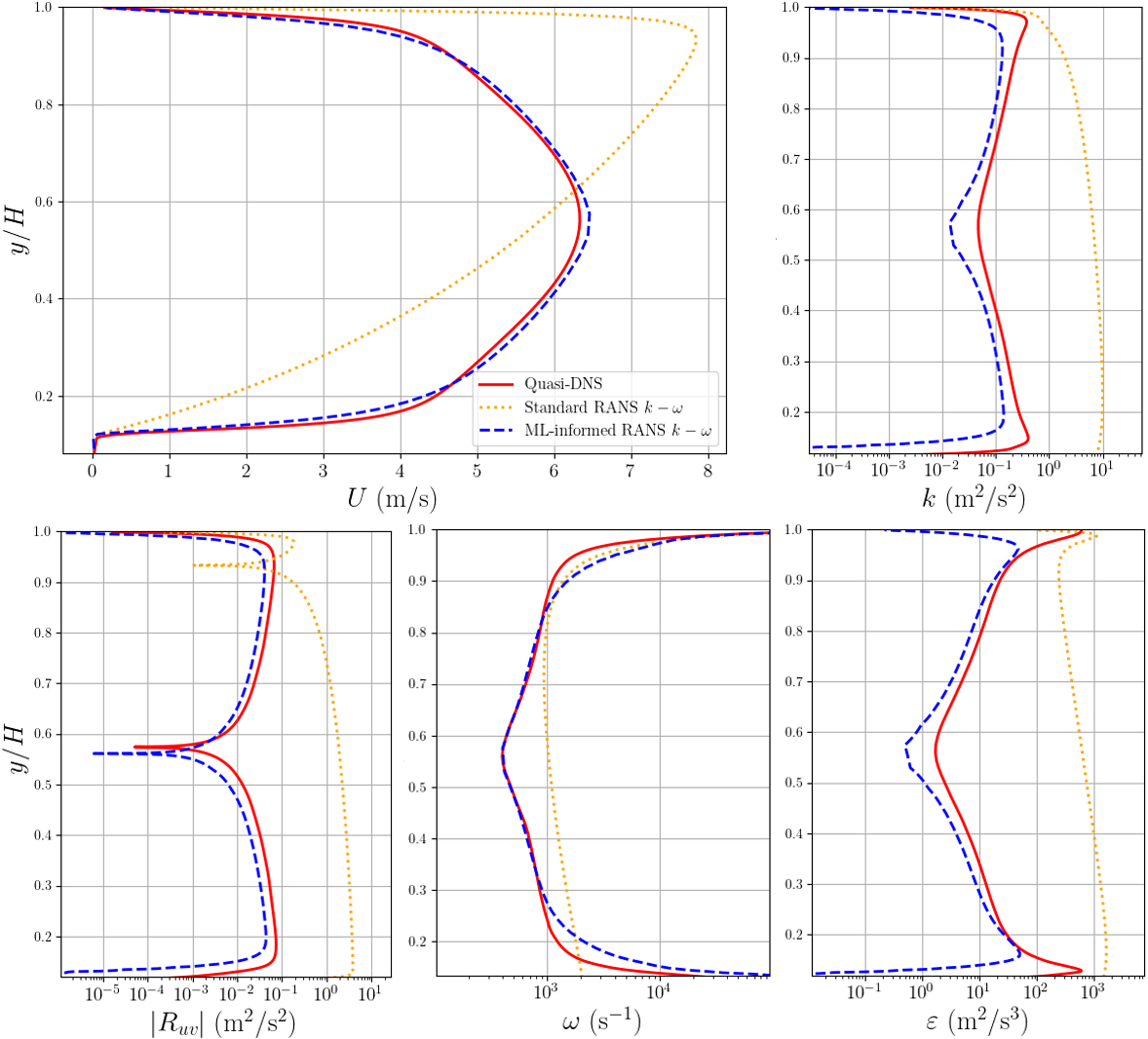
The next step consists in investigating how well a trained ML model perform with different (but relevant) data from the simulated case. Figure 6 shows a comparison between the qDNS, the standard and the new ML-informed RANS simulations of the three configuration 2 test cases. This time five quantities were compared: the mean axial velocity, TKE, Reynolds stress, specific turbulence dissipation rate ω and turbulence dissipation ε. Only two of the three test cases are compared in Figure 6 for clarity: cfg.2-1 and cfg.2-2. Results of cfg.2-3 are shown in Figure 8, Appendix A. For the regime of the liquid phase being laminar (cf. Table 1) results focus on the gaseous phase of the flow. On the one hand, it is observed that the standard k−ω model performs rather very badly for the five quantities plotted in Figure 6. The same shift of the velocity is observed as well as a shift in the stress profile also towards the upper wall of the channel, as previously observed in configuration 1. On the other hand, the ML-informed k−ω model matches the qDNS results very well for the two test cases overall, especially for the velocity, for the stress, and evidently for the specific turbulence dissipation rate which is directly corrected by the ML model in the equation for the transport of ω.

Figure 6.

Comparison between qDNS, standard and ML-informed RANS k−ω of the mean axial velocity (top left), TKE (top right), shear stress (bottom left), specific turbulence dissipation rate (bottom centre) and turbulence dissipation (bottom right) in the gaseous phase for cfg2-1 and cfg2-2.

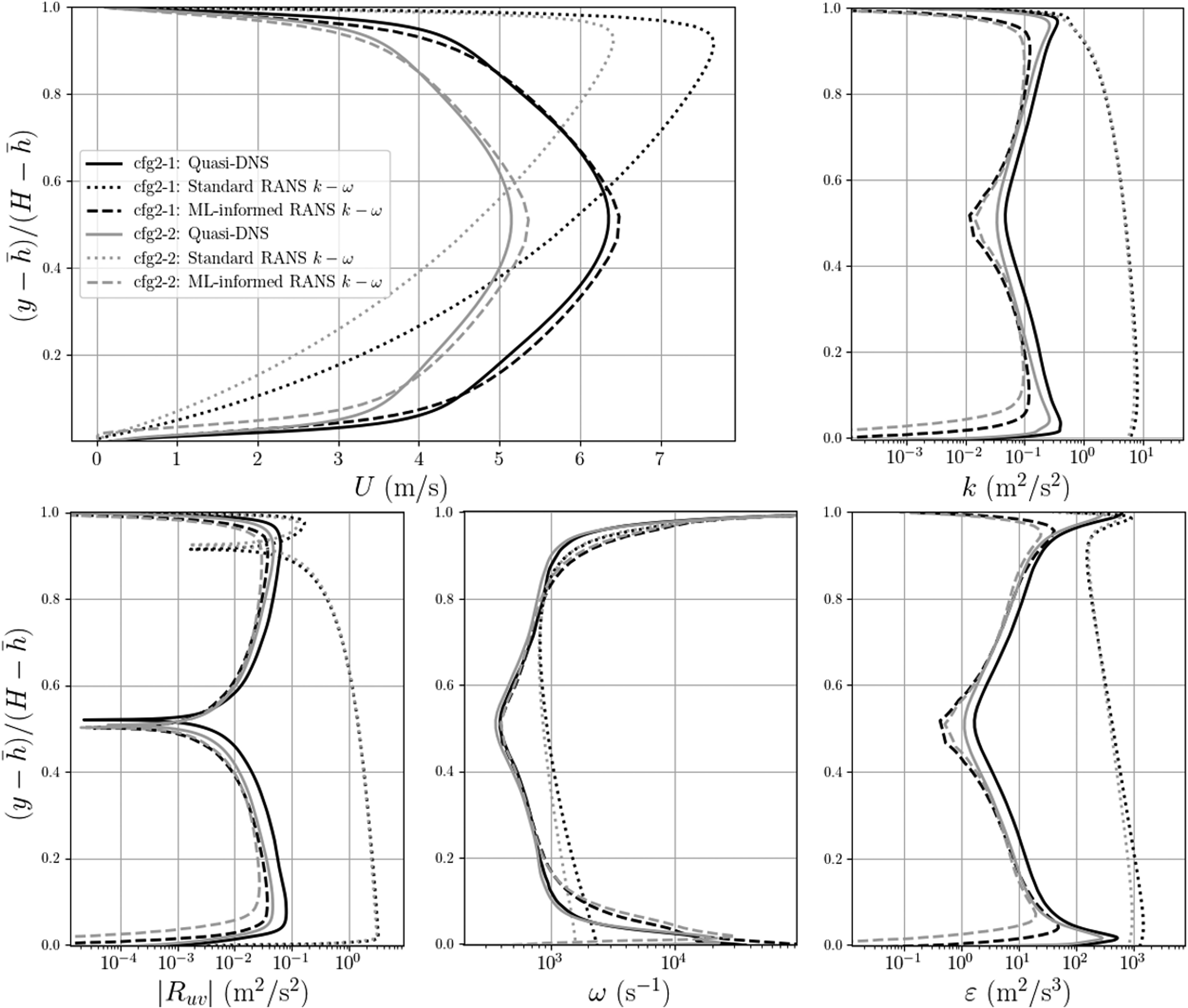
The ML-informed turbulence model slightly underestimates the TKE and turbulence dissipation rate in the centre of the channel and results are slightly closer to the qDNS for cfg.2-2. This would mean that the trained model might perform better for slightly lower speed regimes. Results of cfg.2-3 as shown in Figure 8, Appendix A also match the qDNS data very well for all quantities using the ML-informed k−ω model, compared to the standard k−ω model. For the most turbulent cases, the ML-RANS k−ω model extended the computation time by 28% in comparison with the standard RANS k−ω model.

Overall, the ML-informed RANS simulations performed very well in contrast to standard RANS. Some improvements could be made by expanding and/or better balancing the training dataset for the ML model. Diversifying the cases may help the ML model to adapt to other different configuration too. Finally the ML model might benefit from additional input flow features such as spatial features (distance from the interface, distance from the wall).

Conclusions

In this paper, a novel approach for RANS modelling of two-phase co-current shearing flows was studied. This approach was developed as an alternative to the Egorov’s turbulence damping method (Egorov et al., 2004) that is mesh dependent and lack of guidelines for its use, which makes it case dependent as well. It was showed that a budget correction for the transport of ω in the RANS k−ω turbulence model can be predicted by a simple FFNN machine learning model trained with appropriate qDNS data. By only taking 3 inputs for the NN, the model was able to achieve good prediction of the source term to add into the ω transport equation. A proof of concept was firstly carried out in the configuration of a deep water channel flow using the predictions of a ML model trained on the same flow conditions as the tested case. In this first use of the ML model to inform the budget of the transport specific turbulence dissipation rate, very good agreement was found between the corrected RANS and the qDNS and experimental measurements for the three compared quantities i.e., the mean axial velocity, the turbulent kinetic energy and Reynolds stress. This method was then used to apply appropriate corrections for new cases in a shallow water channel configuration, and using a ML model trained with a variety of qDNS simulations at a range of different flow conditions. The ML-informed RANS k−ω model performed much better than the standard RANS k−ω model with results very close to the qDNS for the three test cases. The mean axial velocity, turbulent kinetic energy, Reynolds stress, specific turbulence dissipation rate and turbulent dissipation profiles were compared. However, some small discrepancies were found in the centre of the gaseous phase in those test cases, where the ML-informed RANS slightly underestimated the TKE and turbulence dissipation rate. Those differences were found to be reduced for the lower speed case.

The promising results of the approach presented in this paper encourage further studies using machine learning as a tool to inform the interfacial turbulence in two-phase shearing flow simulations. Using a much larger dataset containing many cases with various flow conditions, the machine learning model would benefit from a higher quantity and more balanced training. The structure of the neural network could also be revised by changing the number of input features, hidden layers and neurons for example. Adding space related inputs to the model may increase the prediction accuracy. Further research could also investigate other open channel configurations.

Nomenclature