
Introduction
In most situations, the fan or compressor has to be worked under inlet total pressure distortion. Numerous researches have shown that the inlet total pressure distortion has a substantial impact on an engine's efficiency and stability margin. Therefore, it is crucial to reveal the underlying flow physics inside fan or compressor when inlet total pressure distortion presented.
The body force modeling method (BFM) has already been applied to inlet distortion problems in the literature. Due to the relatively coarse grid was used, the BFM predicted the overall performance of compressor subjected to inlet total pressure distortion very quickly (Hale, 1996; Chima, 2006). However, it was necessary to establish a proper body force model when simulating the transonic compressor flows with inlet distortion (Thollet et al., 2016). Hall et al. adopted the BFM to predict the flow in the low speed fan subjected to inlet distortion resulted from boundary layer ingesting (BLI). The results illustrated that nonaxisymmetric stator, increased stage flow and stagnation enthalpy rise coefficients can offer the most potential for improving the performance of BLI fan (Hall et al., 2017). These models are of great value for performance evaluation, but low-fidelity for revealing unsteady flow physics. Yao et al. validated the capability of using unsteady RANS method (URANS) to simulate the distortion flow in multistage transonic compressor, and compared to the experimental data (Yao et al., 2010a). The results lead to thorough understanding of the total pressure distortion transfer and the generation of the total temperature distortion (Yao et al., 2010b). Then Fidalgo et al. applied URANS to simulate flow in NASA rotor 67 with inlet total pressure distortion covers a sector of 120 degree (Fidalgo et al., 2012). A streamline post-processing method has been proposed to estimate the fan performance. They found that the redistribution of upstream flows lead to a variation in work input around the annulus, that determines the distortion pattern downstream of the fan. Simulating NASA rotor 67 with the same distortion pattern as used by Fidalgo, Zhang et al. discovered that the stall margin reduces as the corrected speed decreases (Zhang et al., 2020). Gunn and Hall adopted URANS to simulate the distortion flows of a low-speed fan rig and a transonic fan under the same representative BLI inlet velocity profile (Gunn and Hall, 2014). The distortion flow field was shown to create the circumferential and radial variations in diffusion factor with a corresponding loss. And the transonic fan contains the same flow features as the low-speed fan, except the variations in shock structure induced by BLI. Page et al. found that inlet total pressure distortion would cause the most significant reductions in stall margin of compressor (Page et al., 2018). Although URANS is the most accurate method to simulate the unsteady flow patterns with inlet distortion, it is very time consuming and difficult to be used during the daily design process.
In the past decade or so, several Fourier based reduced order method has been developed to simulate periodical unsteady flows in turbomachinery. Li and He developed a shape correction phase-shifted method and applied to simulate a transonic fan under circumferential inlet distortion (Li and He, 2001), then 5 times speed-up was achieved compared to the traditional multi-passage time marching simulations. He and Ning proposed the nonlinear harmonic method (NLH), in which the time-averaged equations and unsteady perturbation equations were coupled and marched in pseudo time simultaneously (He and Ning, 1998). Mehdizadeh et al. applied the NLH method to simulate the unsteady flows of NASA stage 67 subjected to a square inlet distortion profile (Mehdizadeh et al., 2019). The NLH method offered a cost saving of two orders of magnitude compared to the traditional URANS simulation. Hall et al. proposed the harmonic balance method (HB), in which the time dependent flow variables were approximated by truncated temporal Fourier series (Hall et al., 2002). Peterson et al. used the harmonic balance solver in STAR-CCM++ to simulate a transonic fan stage under a total pressure distortion covered a sector of 90 degree (Peterson et al., 2016). The results demonstrated the harmonic balance method can capture the process of distortion transfer, and obtain 5–7 times computational cost saving compared to the full annulus simulation. However, the HB method is incapable of capturing the far upstream wakes in multi-stage compressor. To overcome the limitations of HB method, Wang et al. proposed the coupled time and passage spectral method (Wang et al., 2021). By including the inter blade phase angle and passage index in the truncated Fourier series, this method can deal with zero frequency harmonics and time harmonics with same frequency but different inter blade phase angles. Based on the differential quadrature method, Du and Ning proposed the time collocation method (Du and Ning, 2013), and the cubic-spline based time collocation method gave almost identical results to the HB method. This method is several times faster than conventional time marching method in simulating periodic transonic flows for aeroelastic analysis (Du and Ning, 2016). Based on the previously proposed time collocation method, we developed a time-space collocation method which can simultaneously handle the rotor-stator interactions and unsteady interactions which is relatively stationary in space, such as inlet distortion and clocking effects. In this paper, the principle of the time-space collocation method is described and then validated by simulating the unsteady flows in a two stage compressor with inlet total pressure distortion.
Methodology
Time-space collocation method
The semi-discretized integral form of Navier-Stokes equations can be written as
where V is the volume of control cell, Q is the vector of conservative variables,
For the temporal periodic flows in turbomachinery, the conservative variables Q can be approximated by a truncated temporal Fourier series
where
In order to consider the variation of time averaged flow field in different blade passages, the spatial harmonics are introduced. The time-averaged quantity
where
(6)
In addition, Equation 6 can be written in a more compact form as
where
Time space sampling
In the time-space collocation method, one of the most important issue is the selection of time instants and passage index. According to the previous studies, the the condition number of the inverse Fourier transform matrix of the selected time instants and passage index should reach a small value, otherwise the calculation will be divergent. An optimization algorithms named modified Gram Schmidt process has been used (Guédeney et al., 2013). In this paper, the passage index ranges from 1 to the blade counts in the studied row. When determining the time instants, the longest period of considered disturbances in the studied blade row is expanded by 500 times, and then firstly divided into
Boundary conditions
The phase-shift boundary condition is adopted in the time-space collocation method to use computational domain of a single blade passage. As shown in Figure 1, The flow variable at interior cells along the lower periodic boundary can be given as
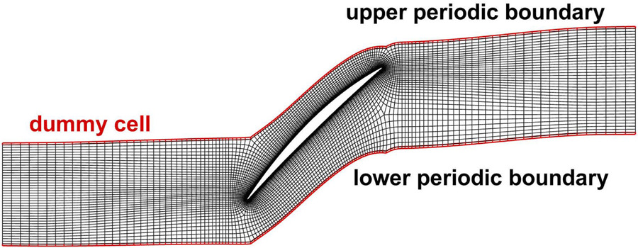
The flow variable at dummy cell along the upper boundary can be updated as
where
The time-space collocation method (TSC) has been implemented in an in-house CFD code named MAP (Multi-purpose Advanced Prediction code for fluid dynamics), which has been extensively validated in simulating turbomachinery flows (Ning, 2014). MAP solves the Reynolds-Averaged Navier-Stokes equations on structured grids, based on cell-centered finite volume method. The advective flux is discretized by LDFSS scheme which is one of the AUSM-family schemes and performs quite well in the viscous and shock wave-containing flows (Edwards, 1997). The MUSCL interpolation with minmod limiter is used to achieve high orders of spatial accuracy and guarantee monotone solutions close to discontinuities. The diffusive fluxes are evaluated using the conventional central differencing scheme. And the one-equation Spalart-Allmaras turbulence model is applied for turbulent flows (Spalart and Allmaras, 1992).
Results and discussion
Test case
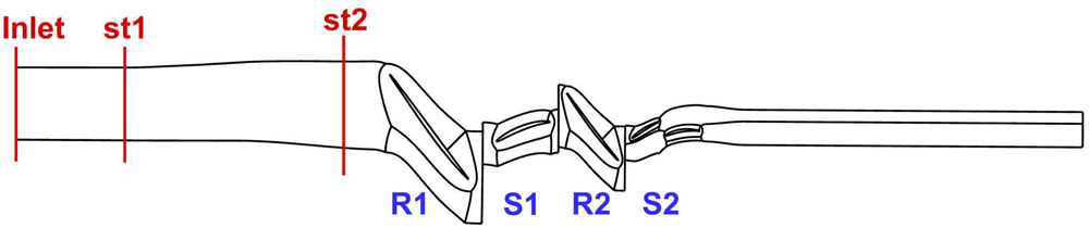
The propagation of inlet total pressure distortion through a two-stage compressor is simulated to verify the proposed TSC method. As shown in Figure 2, the compressor contains four blade rows, including one tandem stator blade row. The rotating speed is 13,266 rpm. Figure 3 shows the computational mesh at the 70% span that is generated by an in-house code named Turbomesh, which is primarily designed to automatically generate structured mesh for turbomachinery flow simulation (Ning, 2014). The O-3H mesh topology is used for a single blade passage, and the grid size for each blade passage and blade counts are listed in Table 1. The overall mesh size of single passage is about 2.25 million.

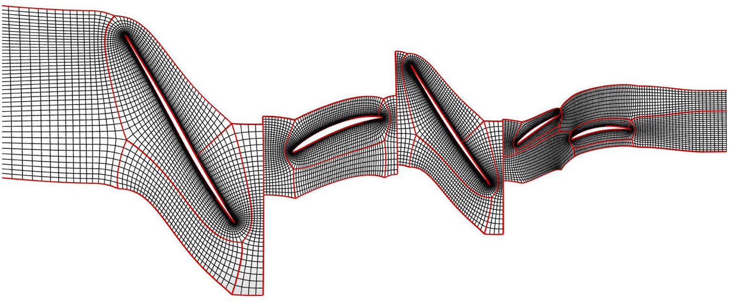
Table 1.
Blade number and grid size of single passage.
| Blade row | Blade number | Grid size (106) |
|---|---|---|
| Rotor 1 | 19 | 0.73 |
| Stator 1 | 42 | 0.30 |
| Rotor 2 | 29 | 0.52 |
| Stator 2 | 54 | 0.70 |
Figure 4 depicts two total pressure distortion patterns representing the typical distortion patterns in experiments, which are specified at inlet boundary. The distortion patterns compose circumferential and radial non-uniformity, which are generated by inserting a plate in a straight pipe. In order to study the effect of distortion intensity on the compressor's performance, the Pattern-H contains larger regions with low total pressure than the Pattern-L. Meanwhile, the total temperature remains uniform and the circumferential flow angle is set to be zero at the inlet.
Quasi-3D flow at 70% span
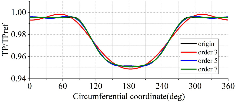
Firstly, a quasi-3D section of 70% span of this compressor is simulated for fast comparison purpose. And the quasi-3D computational domain is depicted in Figure 5, including two monitoring stations named st1 and st2, respectively. Figure 6 depicts the total pressure distortion profile specified at the inlet which is extracted from the Pattern-L as displayed in Figure 4, and the total pressure profile reconstructed by different harmonics of Fourier series are also plotted. It implies that the total pressure distribution approximated by only considering the first three harmonics could matches the specified inlet total pressure distortion pattern very well.
One of the purposes of this work is to identify the influence of harmonic orders adopted in the TSC method, hence the TSC simulation with the first three, five, and seven harmonics of the inlet total pressure distortion considered and without considering blade row interactions were performed. Besides, the extra disturbances induced by adjacent blade row interactions was considered by using the first three harmonics of the blade passing frequency to further assess its impact on the distortion transfer process. As a comparison, an URANS simulation of the inlet total pressure distortion was also performed. The number of physical time steps per revolution was set to be 950, and 20 sub-iteration steps in one physical time step was adopted. The five quasi-3D simulation cases have been carried out on a personal computer with 24 cores (3.0 GHz). To investigate the computational time consuming of TSC as compared to URANS, a simple speed up factor can be defined as following
where
Firstly, the total pressure ratio and isentropic efficiency characteristic of the compressor under clean and distorted inlet flow are shown in Figure 7. There is no obvious differences between the overall performance calculated by the TSC method with different harmonics considered. At the same mass flow rate, the isentropic efficiency calculated by the TSC method deviate from the results of URANS simulation by only 0.3%. When the additional three time harmonics are employed to consider the rotor-stator unsteady interactions, the efficiency characteristic is very close to the results of URANS simulation.
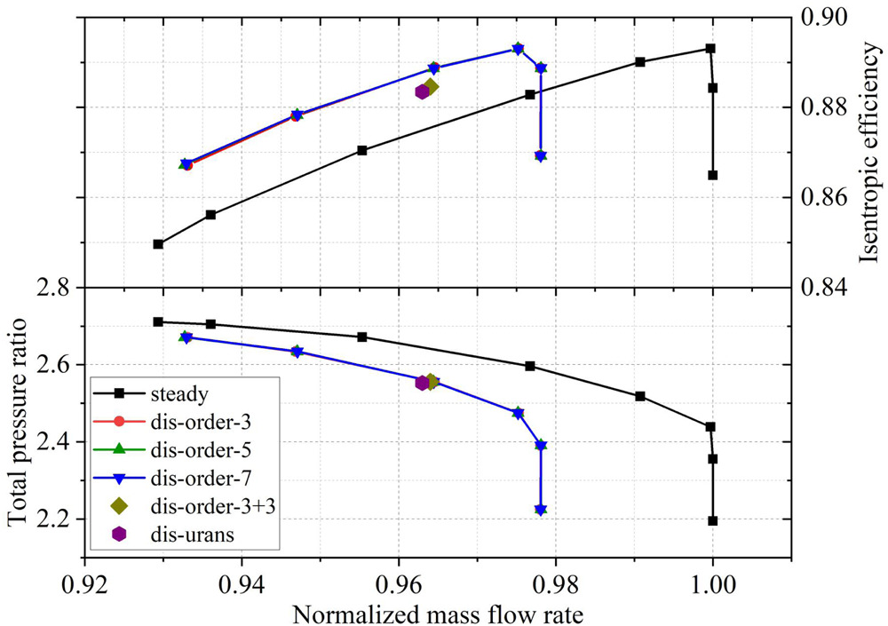
Figure 8 depicts the efficiency convergence history of these five simulations. Notably, the convergence history of URANS simulation only shows the results at the physical time steps. The URANS simulation reaches a well-posed periodical state after three revolutions, and the actual number of iteration steps is as high as 57,000. As expected, the TSC simulations need much fewer iteration steps to approach a quasi-steady state. As shown in Table 2, compared to the reference URANS simulation, the TSC simulations consume much less CPU time. And the TSC gains about two orders of speed-up when three spatial harmonics are considered.
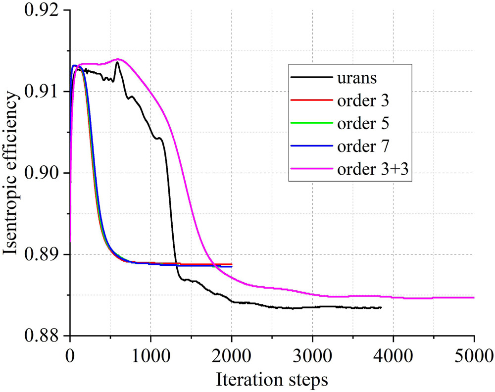
Table 2.
SPF of each simulation case in quasi-3D cases.
Figure 9 depicts the circumferential distributions of the nondimensional axial velocity, static pressure, and swirl angle at two positions upstream of Rotor 1, and the location of these two axial planes are shown in Figure 5. The compressor faces an nonuniform axial velocity distribution around the annulus when subjected to inlet total pressure distortion. The TSC results are quite compatible with those obtained by URANS simulation. As can be seen, three spatial harmonics adopted in the TSC method are sufficient to capture the distortion flow patterns upstream of the compressor. And adopting five or seven spatial harmonics in the TSC method only slightly narrows the distortion region, which is to be expected when high order harmonics are contained.
Figure 9.
Normalized axial velocity, static pressure and swirl angle distribution at two axial position.
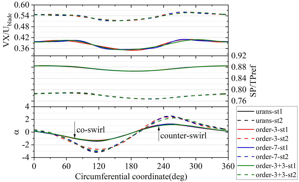
The distorted region contains lower mass flow, which pushes the local operating point to higher pressure ratio, inducing a static pressure field imbalance upstream of the compressor. The gradient of static pressure drives the flow moves from undistorted region to distorted region, and forces the mass flow distribution to be more uniform, that is clearly visible from the axial velocity and swirl angle distribution at st2. The same flow redistribution is revealed by TSC solution with different harmonic orders as compared to the reference URANS solution.
The instantaneous entropy contours are displayed in Figure 10, which can illustrate the transportation of distortion within the compressor blade rows. For the reference URANS simulation, the distortion region with high entropy has been shifted by a phase angle in the rotation direction at the outlet of compressor. As previously mentioned, the compressor must confront co-swirl and counter-swirl flow when it enters and exits the distortion region (as shown in Figure 9). As a result, the blade's local operating point is different around the annulus, which causes the blade loading to be varied across the blade passages. Thick wakes generated by the high loading blades in the distorted region interact with the distortion flows and expand the high entropy region.
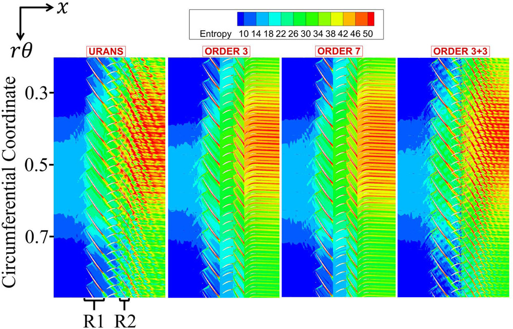
The phase shift phenomena is revealed by the TSC solution with three and seven spatial harmonics, but it also tends to narrow the compressor's high loss region downstream of compressor. The wake convection can be resolved when adjacent rotor-stator interactions are taken into account, producing roughly the same range of high entropy region compared to the URANS solution. This also explains why the efficiency decreases when three harmonics of rotor-stator interactions are considered.
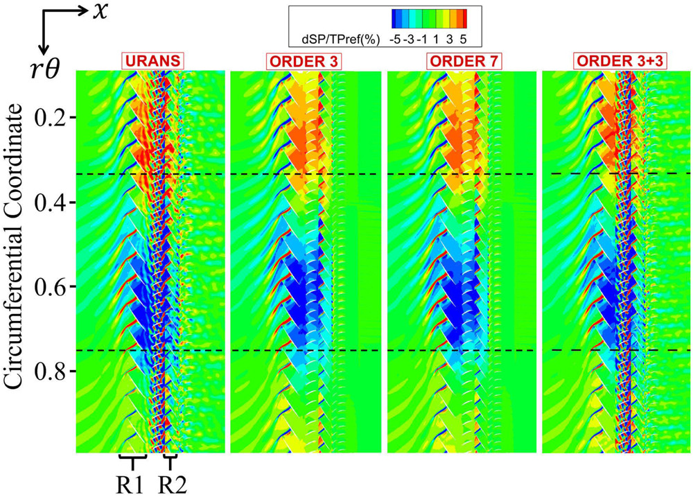
The rotor blade travels in and out of distorted region periodically, inducing the high static pressure perturbations on the blade surface. The instantaneous static pressure perturbation field is depicted in Figure 11. When the rotor enters into the distorted region, the co-swirl flow tends to reduce the incidence, resulting in lower static pressure rise in the blade passage. However, when the rotor leaves the distorted region, the counter-swirl flow tends to rise the incidence, which leads to higher static pressure rise. The above static pressure perturbation phenomenon around the annulus is captured by the TSC simulation with three and seven spatial harmonics. It is important to note that the high static pressure perturbations in Stator 1 has not been captured unless three extra harmonics of rotor-stator interactions were contained in the TSC simulations. This demonstrates that considering the adjacent rotor-stator interactions is important to accurately simulate the pressure perturbation, but not so important for the resolution of distortion transfer.
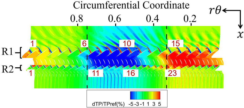
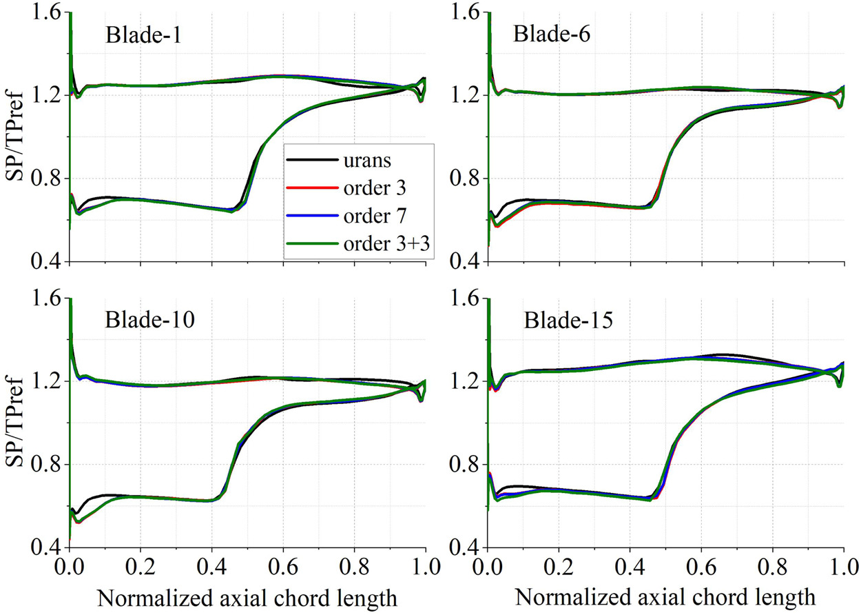
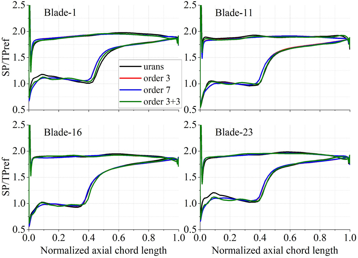
The instantaneous total pressure perturbation distributions are shown in Figure 12 and the instantaneous static pressure distributions on some blade surfaces in Rotor 1 are shown in Figure 13. As depicted in Figure 12, Blade-1 is in the undistorted region, Blade-6 is entering the distorted region, Blade-10 is in the middle, and Blade-15 is leaving out. It is visible that the incidence angle of the TSC simulations is larger compared to URANS, thus the static pressure at leading edge of suction side is a little lower. However, it can capture the shock position and static pressure in other regions precisely. And the static pressure distribution on Rotor 1 blades does not be improved when three harmonics of stator 1 potential interactions were considered. Figure 14 depicts the instantaneous static pressure distribution on blade surface in Rotor 2. As depicted in Figure 12, Blade-1 is in the undistorted region, Blade-11 is entering the distorted region, Blade-16 is in the middle, and Blade-23 is leaving out. Similar with the results in Rotor 1, the TSC simulation only with inlet total pressure disturbance tends to lower the static pressure at leading edge, and there is a deviation of shock position from the URANS solution. For the Rotor 2 blades, they feel the wakes and pressure disturbance from the upstream Rotor 1 and Stator 1 blades, together with the potential disturbance from the downstream Stator 2 blades. The resolution of the static pressure at leading edge and shock position can be improved when three temporal harmonics resulted from rotor-stator interactions are considered. However, minor deviations still exists compared to the URANS simulation due to the nonlinearity of these unsteady interactions.
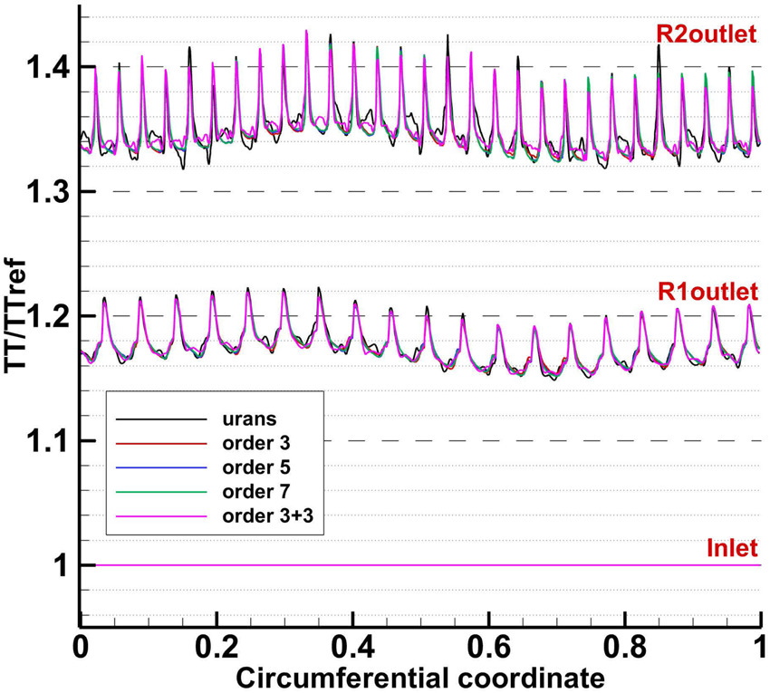
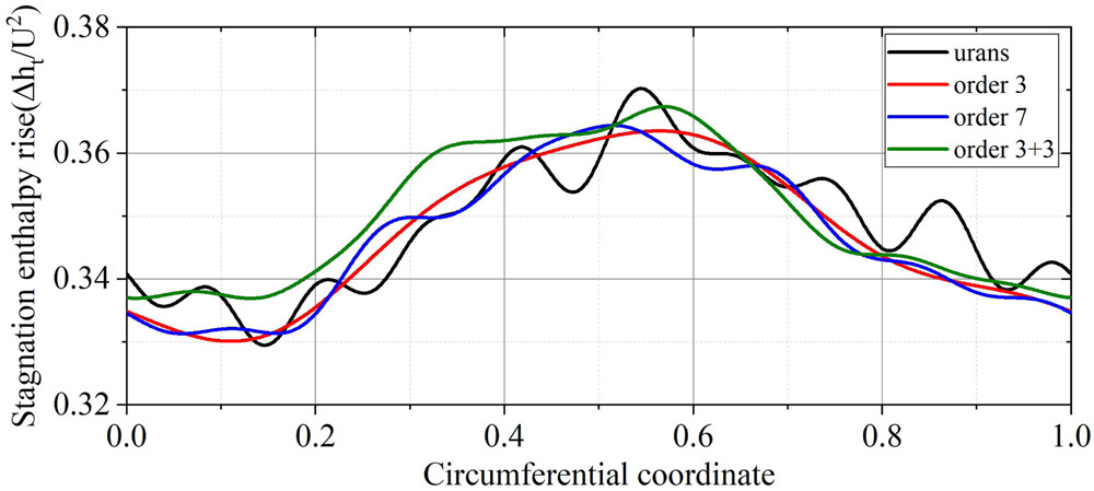
The instantaneous distribution of total pressure and total temperature at three axial positions are displayed in Figures 15 and 16, respectively. The rotor wakes are clearly visible. The total pressure distortion interacts with the blades of Rotor 1 causing the blade loading varied across the annulus, thus producing obvious total pressure and total temperature distortions downstream of Rotor 1. Figure 17 shows the instantaneous stagnation enthalpy rise downstream of Rotor 2, in which the higher-order harmonics have been filtered out. It can be seen that the stagnation enthalpy rise is higher in the distorted region. And it is demonstrated that the blades of Rotor 2 in distorted region contribute more work than blades in the undistorted region, thus producing a more uniform total pressure distribution at the outlet of Rotor 2. However, the total temperature distortion is obvious at the outlet of Rotor 2. Although these TSC simulations capture the primary total pressure and total temperature distribution patterns, there are small deviations that need further investigation.
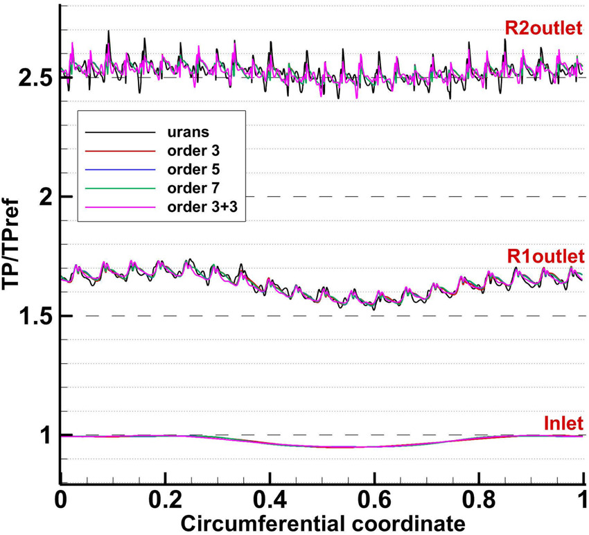
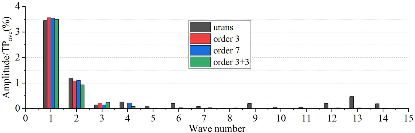
The harmonic spectrum of the total temperature and total pressure distribution downstream of Rotor 1 and 2 are obtained by performing Discrete Fourier Transform (DFT), and the amplitude is normalized by the local averaged values. The majority of perturbation energy is occupied by the first two harmonics, as shown in Figures 18 and 19. The amplitude of the first three harmonics obtained by the TSC with three spatial harmonics is close to the URANS solution. And the resolution accuracy is improved a little when additional spatial or temporal harmonics are retained.
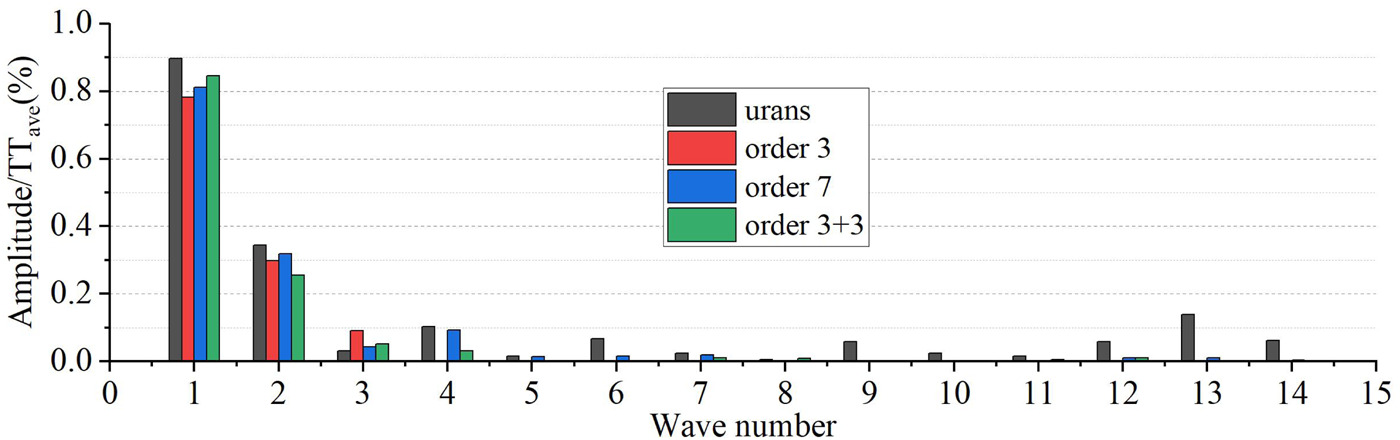
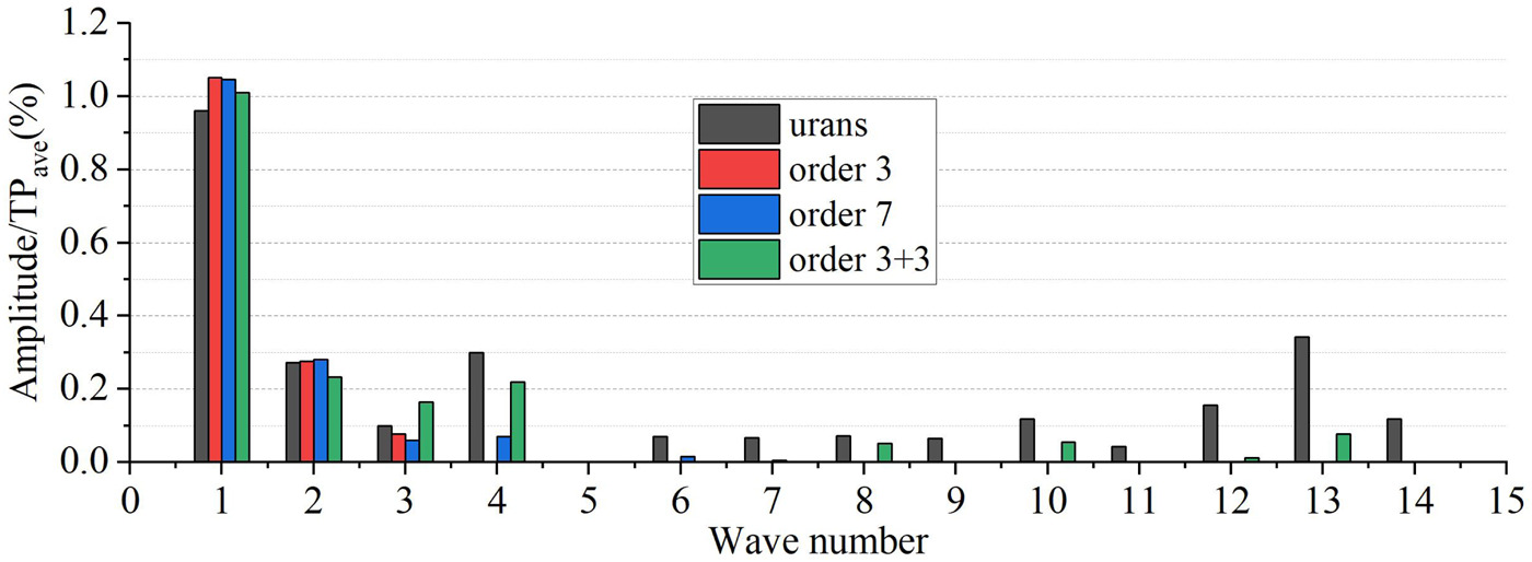
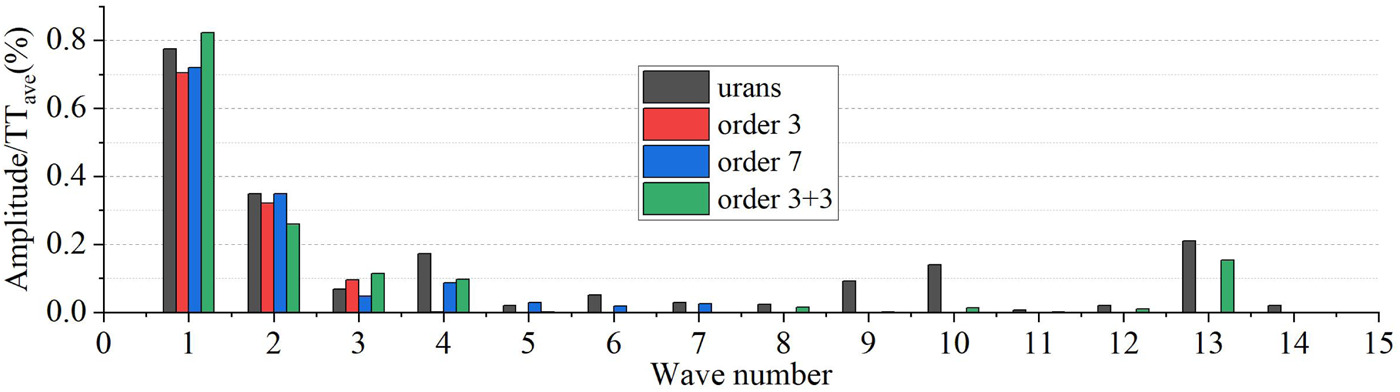
Compared to Figure 18, the amplitude of the first two harmonics has been significantly reduced (as shown in Figure 20), indicating the total pressure profile downstream of Rotor 2 becomes more uniform. However, the generated total temperature distortion indicated by the first three harmonics remain essentially unchanged, as shown in Figure 21. Due to the interactions of wakes and potential disturbance, the amplitude of some perturbations with high wave number cannot be ignored. The TSC with three harmonics of adjacent rotor-stator interactions can capture some perturbations with high wave number, but the improvement is not significant.
Three dimensional configuration
The two stage compressor subjected to inlet total pressure distortion is studied in this section. Firstly, the steady simulation with clean inlet condition was carried out. The normalized steady characteristic shown in Figure 22 matches the experimental results very well. Then the TSC with only five spatial harmonics was used to simulate the compressor flow subjected to inlet total pressure distortion, as denoted as Pattern-L and Pattern-H (in Figure 4). For the purpose of comparison, the URANS simulations with these two distortion patterns were also performed. As similar with quasi-3D case, the number of physical time steps per revolution was set to be 950, and 20 sub-iteration steps in one physical time step was adopted. The five 3D simulation cases have been carried out on a service computer with 112 cores (3.8 GHz).
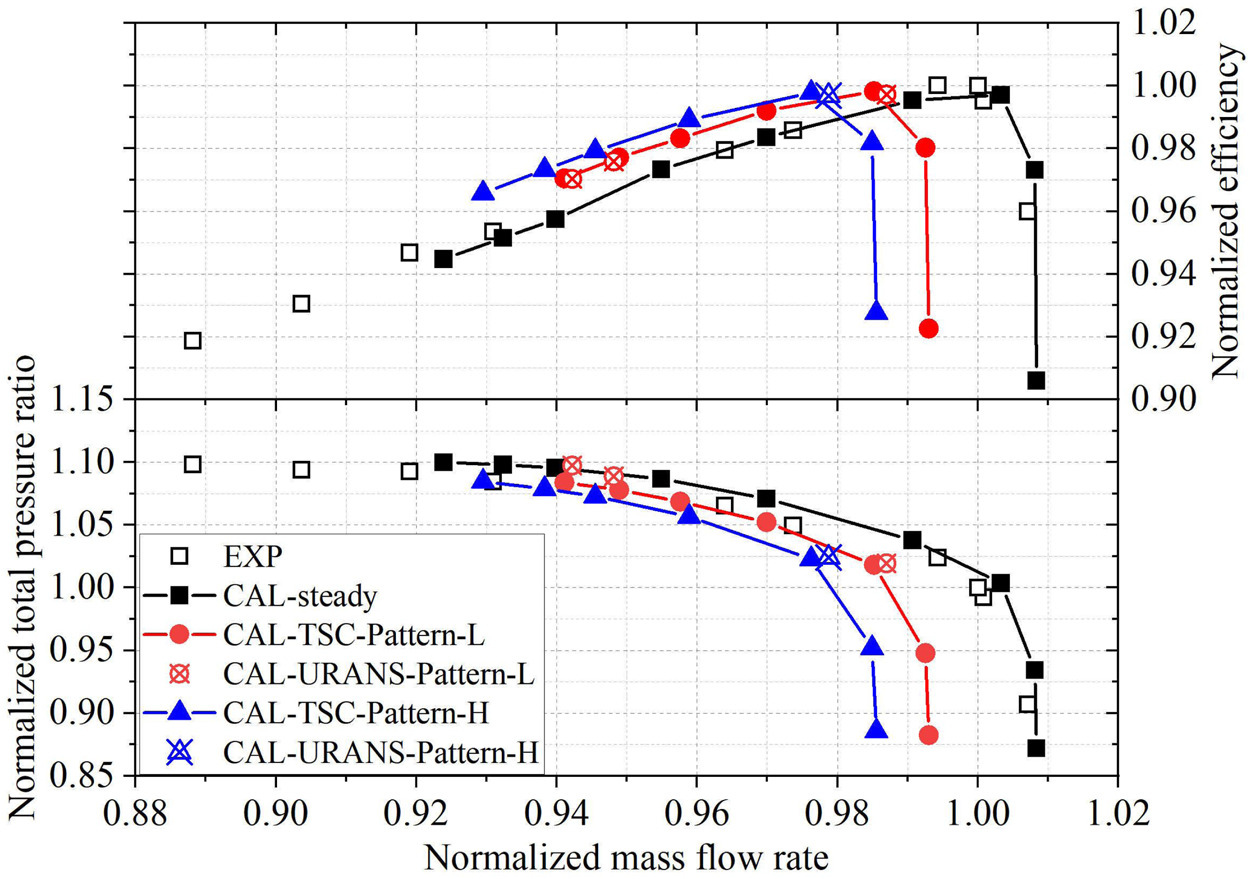
As depicted in Figure 22, the choke mass flow decreases obviously when subjected to inlet total pressure distortion. At the same mass flow rate, the total pressure ratio also decreases but the isentropic efficiency rises a little. The total pressure distortion induces the compressor to stall at higher mass flow rate and a larger distortion intensity results in more degradation of performance. The performance results of TSC agree well with that obtained by URANS at the peak efficiency working point. There is a slight deviation in the mass flow rate, which is only 0.25%. And in the simulation case with Pattern-L, the URANS simulation obtains a well-posed periodic state after three revolutions, but TSC simulation only need 1,000 iteration steps to approach the quasi-steady state. As shown in Table 3, the TSC simulation consumes much less CPU time, and gains about an order of speed-up. Near the stall boundary, two URANS simulation cases with Pattern-L have been performed. The physical time steps per revolution and sub-iteration steps were consistent with these used at the peak efficiency working point, and it needed to simulate four revolutions to obtain a well-posed periodic state. The performance results of TSC are also very close to that of URANS results at the near stall point. The TSC tends to underestimate the total pressure ratio, but the percentage deviation is less than 1.2%. Therefore, the TSC method can obtain relatively accurate results in estimating the performance characteristics of this compressor with inlet distortion.
Table 3.
SPF of simulation cases with Pattern-L.
| Simulation case | Iteration steps | computational meshsize (106) | CPU timeconsuming (h) | Speed upfactor |
|---|---|---|---|---|
| URANS | 57,000 | 70.61 | 290.57 | 1 |
| TSC (five spatial harmonics) | 1,000 | 22.08 | 6.32 | 45.98 |
The distortion transfer phenomenon in the compressor is three dimensional, that is much more complicated than the quasi-3D flow analysis in the above section. The peak efficiency working point with Pattern-L is chosen for detail comparisons between the TSC and URANS solutions. The instantaneous mass flux normalized by inlet averaged value and static pressure normalized by the inlet total pressure at undistorted region are shown in Figure 23. It is obvious that the distorted region contains lower mass flux (region A), thus lower static pressure is induced (region B), especially around the hub (region C). The static pressure gradient drives the flow of undistorted region migrates into the distorted region, creating the co-swirl (region D) and counter-swirl (region E) flow regions, as shown in Figure 24. In this figure, the positive swirl angle represents the opposite direction of the rotor rotation. Meanwhile, the fluid in the hub (region H) convects radially to the higher span sector. From Figures 23 and 24, it can be seen that the solution of TSC with five spatial harmonics reveals the complicated flow redistribution upstream of Rotor 1 at st2 as accurate as the URANS solution.
Figure 23.
Comparisons of normalized mass flux and static pressure upstream of Rotor 1 at st2. (a) URANS (b) TSC (five spatial harmonics).
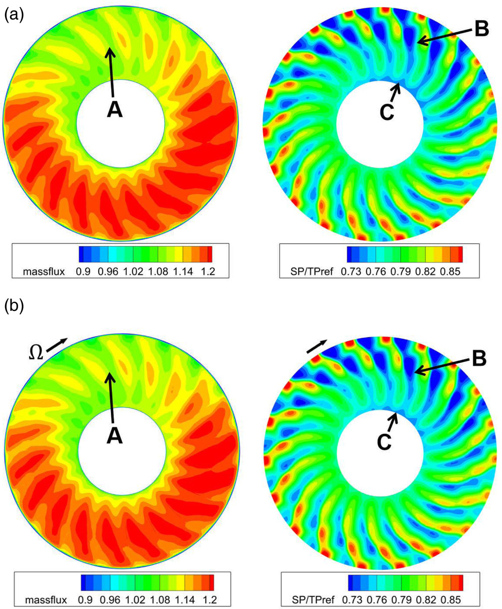
Figure 24.
Comparisons of swirl angle and radial angle upstream of Rotor 1 at st2. (a) URANS (b) TSC (five spatial harmonics).
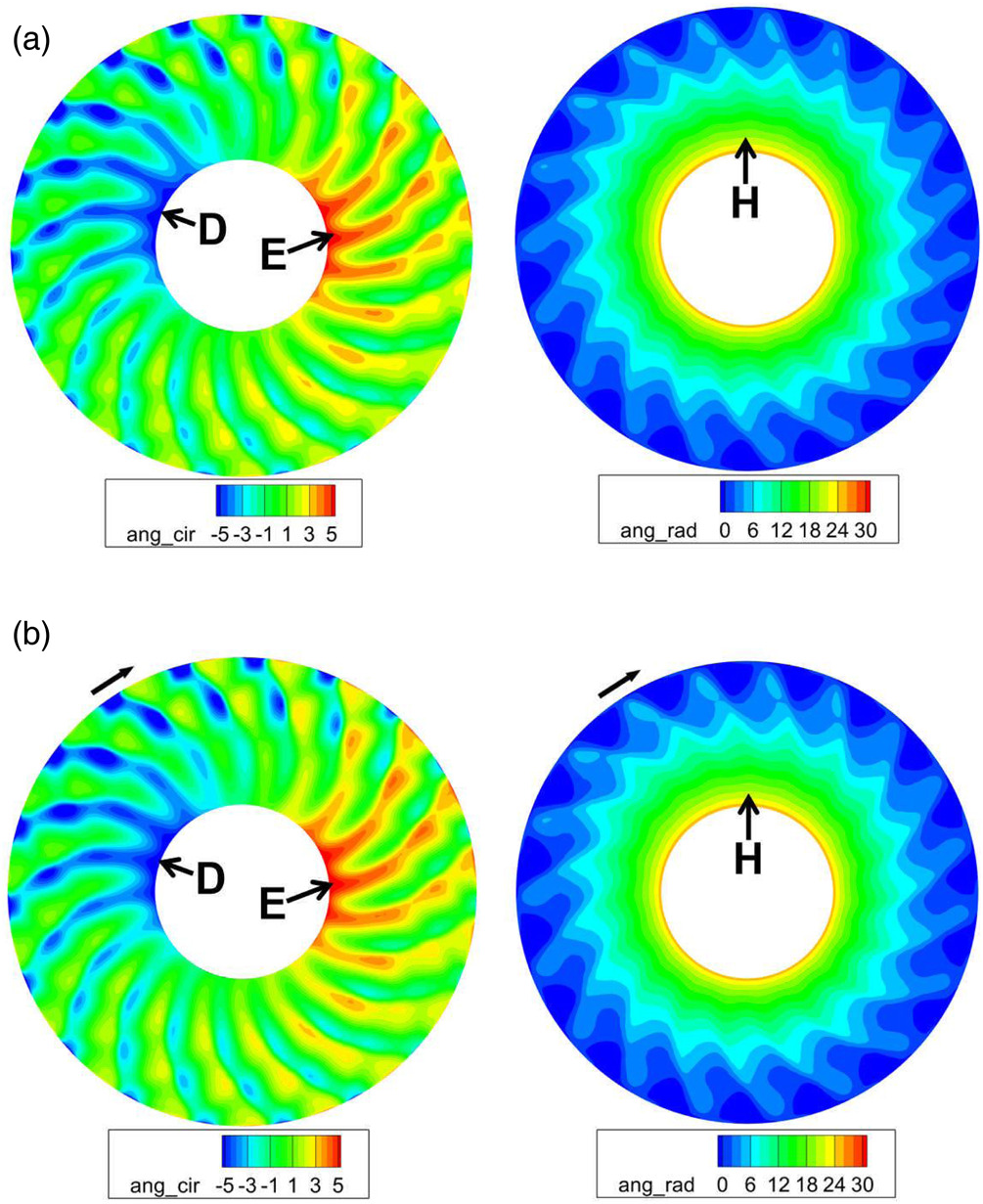
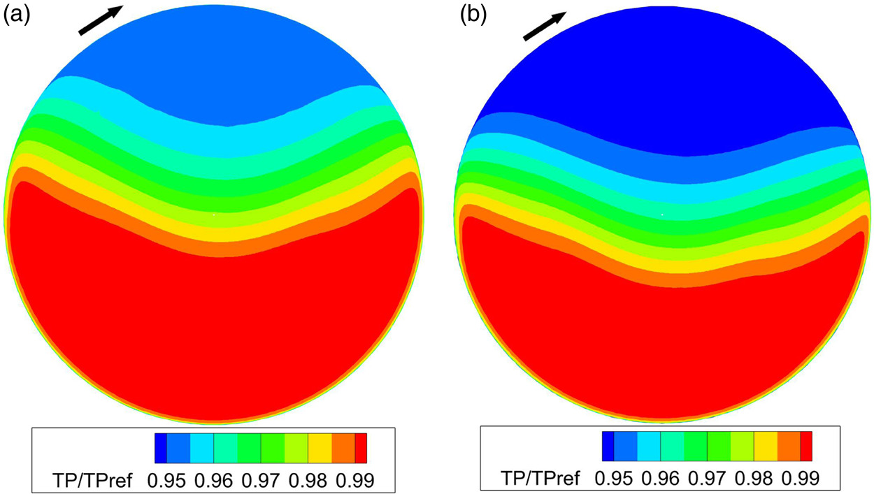
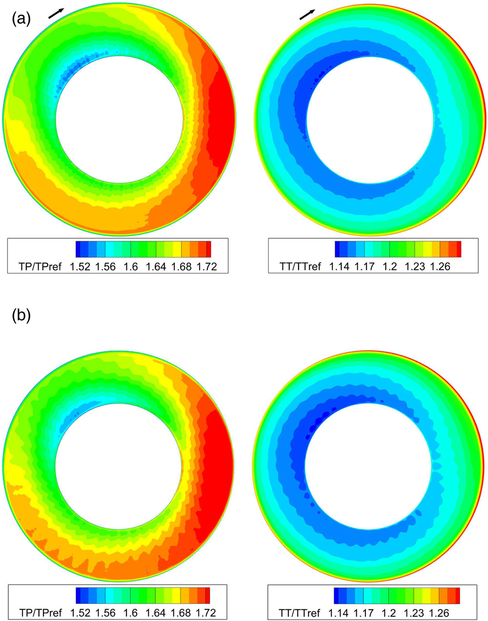
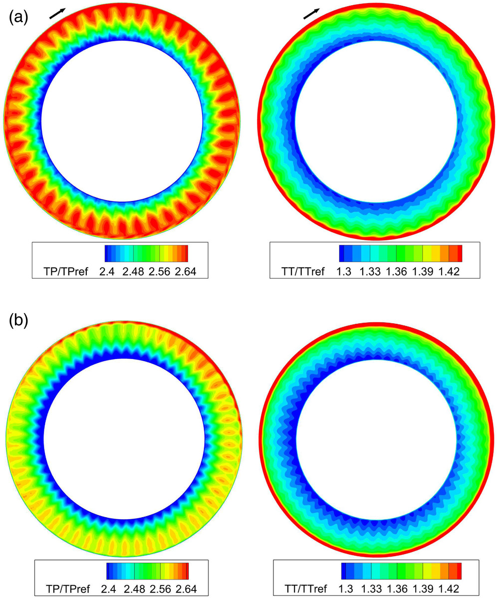
Figure 25 depicts the instantaneous normalized total pressure and total temperature at the downstream side of the R1-S1 interface. Since the disturbance of rotor-stator interactions were not contained in the TSC simulations, the wakes of rotor blades are invisible at the downstream side of the R1-S1 interface in the TSC solution. Due to the interactions of distorted flows and rotor blades, the nonuniform total pressure and total temperature patterns are consequently generated downstream of Rotor 1. When the blades of Rotor 1 travels into the distorted region, it face the co-swirl flow and the incidence as well as work input were reduced, resulting in lower total temperature and total pressure (region A). As shown in Figure 26, the circumferential total pressure distortion is attenuated significantly downstream of Rotor 2, but the total temperature distortion still remains. It can be shown that due to the radial migration of the flow in the hub regions, the radial total pressure and total temperature distortions are obvious downstream of Rotor 2. It can be seen from Figures 25 and 26, the TSC solution with five spatial harmonics considered captures the similar complex flow patterns as the reference URANS solution, thus the performance degradation caused by inlet distortion are well estimated by the TSC method.
Figure 25.
Comparisons of normalized total pressure and total temperature downstream of Rotor 1. (a) URANS (b) TSC (five spatial harmonics).
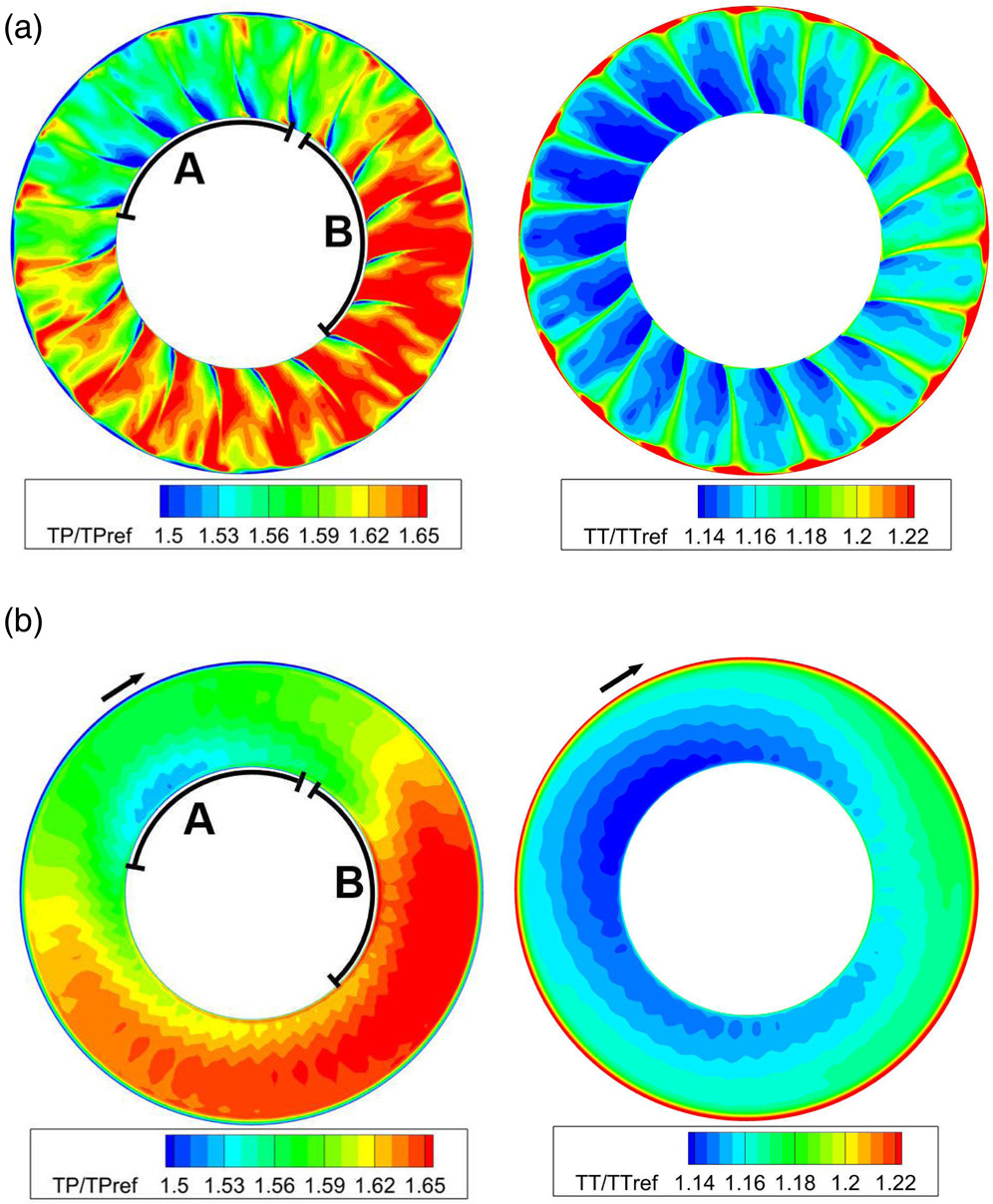
Figure 26.
Comparisons of normalized total pressure and total temperature downstream of Rotor 2. (a) URANS (b) TSC (five spatial harmonics).
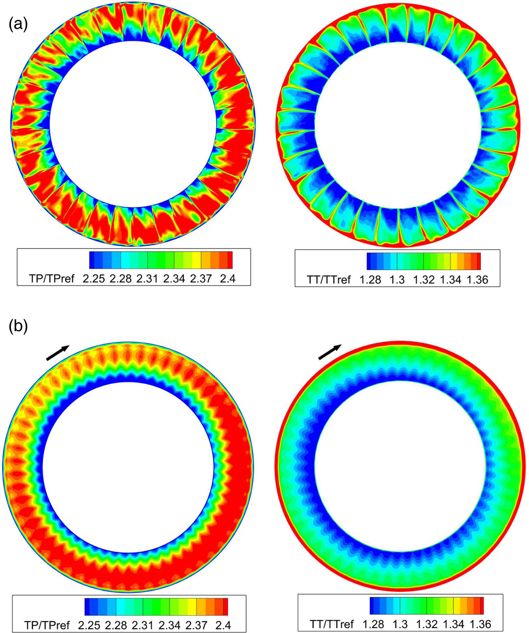
Due to only the spatial harmonics are considered in TSC simulation, the comparisons of instantaneous results indicate some differences in the flow details captured by TSC and URANS. The time-averaged results of URANS in the near stall working point are further compared to the results of TSC in Figure 27. It can be seen that the TSC captures almost the same time-averaged nonuniform total pressure and total temperature patterns downstream of Rotor 1 as the URANS. Figure 28 displays the total pressure and total temperature distributions downstream of Rotor 2. The distribution patterns are similar, but the regions with lower total pressure and total temperature are broader in the solution of TSC than that of URANS, which would be caused by the neglecting of the rotor-stator interactions in the TSC simulation.
Conclusions
For simulating the distortion flow in compressor, traditional time-marching method (URANS) is most accurate, but is extremely time consuming. In order to reduce the computational cost, a novel time-space collocation method (TSC) has been proposed and validated in this paper. Firstly, the flow physics of a quasi-3D two stage compressor operating under circumferential total pressure distortion has been investigated by TSC and URANS separately. The TSC can capture the main unsteady effects due to inlet distortion and can obtain about an order of speed up compared to URANS. The results indicate that only considering three spatial harmonics of inlet disturbance is sufficient to capture the predominant flow pattern subjected to total pressure distortion. Besides, considering the adjacent rotor-stator interactions is important for improving the accuracy of the pressure perturbation distributions calculated by TSC simulation, but not necessary for simulating the propagation process of the distortion flow. Then, the three-dimensional configuration under two typical total pressure distortion patterns has been simulated by TSC and URANS, respectively. The TSC with only five spatial harmonics can capture the performance degradation due to inlet distortion accurately and gains about an order of speed-up. Overall, the time-space collocation method would have promising engineering applications in estimating the performance degradation of fan/compressor subjected to inlet distortion flow.
Nomenclature
Symbols
A,B
Fourier coefficients
C
CPU consuming time (h)
N
number of harmonics
Q
conservative variables
time-averaged quantity
time-space-averaged quantity
R
residual
SP
static pressure
TP
total pressure
TT
total temperature
TPref
reference total pressure, 101,325 Pa
TTref
reference total temperature, 288.15 K
U
blade rotating velocity
velocity
V
cell volume
VX
axial velocity
phase lag angle
wave length
frequency/wave number
stagnation enthalpy rise