Introduction
The use of high-fidelity simulations to analyze turbomachinery flow fields is nowadays a common practice, even at industrial level. Hi-fi simulations may provide a wealth of data for detailed investigation of the flow physics and unveil the dynamics that generate losses. As discussed in the review paper of Sandberg and Michelassi (2022), high-fidelity simulations may be used to extract local information to pinpoint local loss causes. To this end, advanced post-processing methods have been introduced in the last years.
Wheeler et al. (2016) were among the first to show the integral entropy rise in a high pressure turbine blade solved with Direct Numerical Simulation (DNS). They used the entropy transport equation by directly computing the contribution to viscous dissipation by the time-mean strain field and by the turbulence field. Similarly, Miki and Ameri (2022) showed the instantaneous dissipation obtained from Large Eddy Simulation (LES) of a transonic turbine blade. Further detailed analysis of the transport equations of entropy, total pressure or mechanical work potential have been provided by several research groups (e.g., Leggett et al., 2020; Przytarski and Wheeler, 2020; Zhao and Sandberg, 2020; Przytarski et al., 2024b). In these works the losses are evaluated by means of an integral approach within the control volume rather than the classical inlet to outlet loss estimation. With these methods, it is easy to identify where losses are generated. However, it is rather difficult to decouple the dynamical features that lead to the loss generation. In order to overcome this limit, Lengani et al. (2019) applied the Proper Orthogonal Decomposition to LES data of a low pressure turbine blade to identify the most energetic dynamical features. They showed that total pressure transport equation in the Reynolds average sense may be re-written to highlight the contribution of each mode (i.e., dynamical feature). This method has been recently applied to several LPT cases to discern the loss causes (e.g., Dellacasagrande et al., 2023; Russo et al., 2024).
The amount of data that are generated nowadays by LES or DNS easily exceeds tens of terabytes. Therefore, the use of high-performance computing services is becoming necessary also for the post-processing of such simulations. An open source high performance data analytic (HPDA) code, developed within the Euro-HPC ACROSS project, has been described in Biassoni et al. (2024). This open code performs POD on large datasets (tens of TB) and applies the loss breakdown described in Lengani et al. (2019). The present paper provides an extension of these previous work by computing the losses in the Spectral POD (Towne et al., 2018) modal decomposition framework. Among the different open versions of the SPOD (see for example He et al., 2021; Rogowski et al., 2024), the present one leverages on the distributed computation of the Dask framework of Python by providing an ease of programming and good efficiency on multi-node high performance computers.
Methodology
Fundamental equations
Losses of turbomachinery bladings can be evaluated by integrating the substantial derivative of entropy over the computational domain, as one of the most used metrics (e.g., Wheeler et al., 2016; Russo et al., 2024). In most cases, by considering an adiabatic transformation, this operation is equivalent to the integral volume of the substantial derivative of the total pressure with the opposite sign, according to the Gibbs equation (see for example Denton, 1993). Following a Reynolds decomposition approach, the time average of the substantial derivative of the total pressure can be written, adopting Einstein notation, as Przytarski et al. (2024b):
where the equation is written just for simplicity in the incompressible formulation but it may be easily extended to the compressible case by using Favre averaging operation. The overbar indicates the time average operation and the
ui components indicate the mean velocity, while the term
ui′ indicates the fluctuating velocity. The first three terms on the right-hand side correspond to the substantial derivative of the time mean total pressure, whereas the last three terms may be considered in most cases negligible and exceptions to this are discussed in detail in
Przytarski et al. (
2024a,
b). By further neglecting the substantial derivative of the turbulent kinetic energy (
ui′ui′¯), the total pressure variation can be approximated as:
where K is the mean flow kinetic energy. The viscous dissipation due to the mean strain (ϕM) depends just on the time mean flow and the PTKE depends on instantaneous fluctuating velocity. Namely, each instantaneous flow field realization (a snapshot) contributes to the overall time mean value. In particular, in Equation 2, the terms responsible for the largest contribution of loss generation are ϕM and PTKE, as also discussed in Zhao and Sandberg (2020). The overall variation of total pressure (i.e., entropy rise) can be then calculated as the volume integral of ϕM and PTKE:
As discussed in Lengani et al. (2019), it is possible to decompose the contribution to the Reynolds stress tensor (ui′uj′¯) by projecting the instantaneous fluctuating velocity on a complete orthogonal basis. Namely, an orthonormal basis X may be used to decompose the fluctuating velocity field as ui′(x)=Xϕui(x). The modes ϕui are carrying the square root of the energy and provide the spatial representation of the velocity ui′. Considering that the orthonormal basis is in common between the different velocity components, the Reynolds stress tensor may be written as (see also Perrin et al., 2007):
where the time mean operation is initially expressed as the scalar product between the velocity data array, Nt is the number of instantaneous flow field realizations, H indicates the Hermitian transpose and the product XHX is the identity matrix by definition of the orthonormal basis. The Reynolds stress may be then computed as a summation of the spatial modes (note that the complex conjugate conj applies when the modes are complex numbers). Finally, it is possible to compute the turbulent kinetic energy production as Lengani et al. (2019):
In this way, each mode k contributes to a quota of the turbulent kinetic energy production. By finding an optimal base X, it is possible to decouple the effect of the different dynamical features (represented by the modes φ(k)) to the total pressure loss as computed from Equation 3. The application of the POD modal decomposition framework has been developed in several previous papers (e.g., Lengani et al., 2019; Dellacasagrande et al., 2023; Russo et al., 2024) and it is here employed as reference for comparison with the SPOD results. Note that, for this analysis to hold true, it is essential that the orthonormal basis X is common to the velocity components. Consequently, it is necessary to build the data matrix from at least the three velocity components. This operation may result in significant memory requirements for the computation, (e.g., for this limitation Fiore et al., 2023 computed SPOD from a single velocity component by adopting a serial code). The next section describes in detail the new SPOD-HPDA code, that leverages distributed memory among several compute nodes, and presents its scalability results. Two different algorithms for the computation of SPOD modes are used and described.
Python SPOD procedure
This new procedure has been developed in Python by leveraging the Dask (https://www.dask.org/) library for distributed computation. The advantage of Dask is that it is no longer necessary for the user to manually partition domain data to provide parallel computation, since data chunks are automatically managed by Dask. Another advantage of Dask is that you can start from a serial prototype based on NumPy and Pandas libraries and convert it very easily to a fairly large-scale distributed code. For a more complete description of how Dask works, see Viviani et al. (2022).
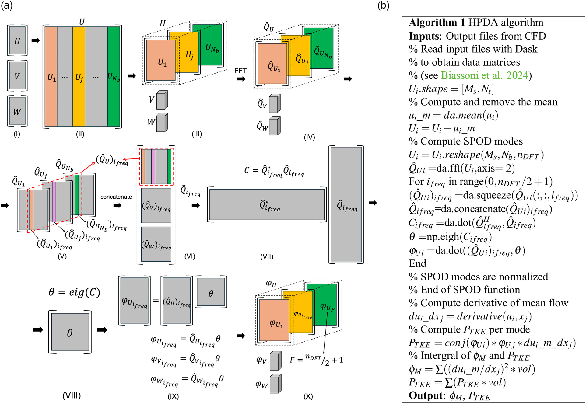
The procedure is visualized in Figure 1a and described in the algorithm depicted in Figure 1b. Please note that our beseline SPOD implementation follows the theoretical formulation of Towne et al. (2018). For the practical “serial” implementation the works of Schmidt and Colonius (2020), He et al. (2021) and Fiore et al. (2023) may be taken as a reference. The common practice of overlapping data in time, typically used in such implementations, is not employed here. This decision ensures a complete orthonormal decomposition in both frequency and SPOD modes. A parallel implementation of SPOD, which overcomes limitations of memory usage and running time, is presented in Rogowski et al. (2024) by utilizing MPI communication between computational nodes. In the present paper, distributed computation is directly managed by Dask, and the variables in the SPOD Kernel are kept separated as much as possible. In detail, the relevant operations managed by Dask are highlighted in the algorithm of Figure 1b with the suffix “da,” otherwise the explicit use of numpy library is indicated with “np.” The output files are read by Dask (see Biassoni et al., 2024) and stored in three data matrices. The three fluctuating velocity components (Ui in the algorithm) are stored in the three data matrices U, V, W (step I of Figure 1a). Each column vector of the matrix retains the spatial information. The rows got dimension Nt (i.e., the number of instantaneous realizations or snapshots), while the columns got dimension Ms, the total number of computational mesh points. The first step of SPOD is fragmenting the time sequence in a discrete number of blocks Nb (step II), which is obtained by means of an array reshape operation (step III). Dask then manages the discrete Fourier transform (DFT) using the FFT algorithm along the temporal direction of size nDFT (with nDFT∗Nb=Nt) to obtain the matrices Q^Ui for each velocity component (step IV). Each 3D array Q^Ui contains the frequency information along its last dimension (shape 2 according to Python indexing, which starts from 0). In the baseline implementation of SPOD, the data for each frequency are then collected within a for loop in order to store the matrices (Q^Ui)ifreq at the frequency loop index ifreq (step V), this operation is done for all variables at hand (step VI). As observed by Rogowski et al. (2024), the number of frequencies of interest is nDFT/2+1, as specified in the algorithm, and this is because of the symmetry properties of the DFT. The matrices (Q^Ui)ifreq are then concatenated to form the Q^ifreq matrix (from step VI to VII) in order to compute the cross-correlation matrix Cifreq within the for loop (step VII) and its eigenvectors θifreq (step VIII). Note that, at present, Dask does not provide the equivalent of the eigenvector calculation of the numpy library and therefore the computation of step VIII is managed by numpy. Nevertheless, the Cifreq matrix is very small with dimension [Nb,Nb]. The SPOD modes are computed separately for each variable as (φUi)ifreq=(Q^Ui)ifreqθ (step IX) and stored in a 3D array (step X) with the same shape of matrices in step III. Finally, to ease the computation of the PTKE, the SPOD modes are reshaped to a matrix with dimension [Ms,Nt]. Namely, SPOD modes are sorted to have first the ordered modes at each frequency index, as it will be better discussed in the result section.
Figure 1.
Spectral-POD procedure: SPOD computational sequence (a); complete HPDA algorithm (b).

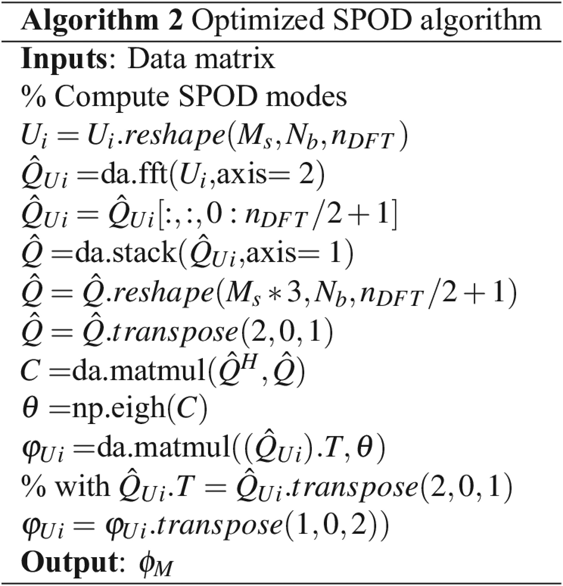
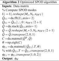
The SPOD computation, detailed in steps V to IX of Figure 1a, has been optimized by eliminating the use of for loops. The improved algorithm, outlined in Figure 2, takes advantage of the execution order in the eigenvector solver from the numpy library. The input data are rearranged using stacking and transposing operations, resulting in a three-dimensional array, C, with dimensions [nDFT/2+1,Nb,Nb]. The first dimension corresponds to the frequency index, and the other two dimensions represent the cross-correlation matrix for each frequency, Cifreq. The numpy function eigh is then applied, solving the eigenvector problem for each Cifreq. This optimization ensures that the output SPOD modes are equivalent to those produced by the baseline implementation.
Figure 2.
Optimized Spectral-POD algorithm with no for loops.
The procedure with the two SPOD implementations is openly available at the following link: https://git.mycloud-links.com/across-public/orchestrator/applications/aeronautics. The online code includes a test dataset and both POD and SPOD procedure for computation of the PTKE.
Scalability tests
Scalability results, concerning the SPOD distributed computation only, are presented here on a relatively large LES dataset. The dataset consists of approximately 80 million computational points and 950 snapshots. Originally stored in CSV files, the snapshots were converted to binaries using the procedure outlined in Biassoni et al. (2024). The binary files (in Parquet format) occupy around 2TB of disk space, as the three velocity variables were stored.
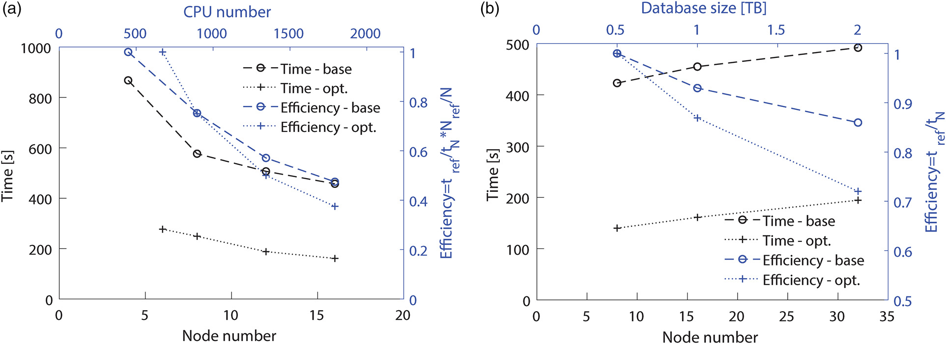
Both strong and weak scalability tests for baseline and optimized SPOD implementations are shown in Figure 3. In the former, the LES database is analyzed with an increasing number of computational nodes to observe the speed-up obtained by increasing the CPUs. Conversely, in the latter, the number of snapshots is progressively increased alongside the number of computational nodes to assess the code efficiency. All tests described here were executed on the CINECA cluster LEONARDO (https://www.hpc.cineca.it/systems/hardware/leonardo/), utilizing the general-purpose CPU partition (DCGP). In brief, each computational node in DCGP is equipped with 2 × 56 Intel Sapphire Rapids cores running at 2.0 GHz and 512 GB of RAM. Strong scalability tests were conducted using a halved snapshot size (Nt=480) to limit the use of resources. The tests have been conducted by setting Nb=10 and consequently nDFT=48, and were repeated at least three times for statistical validity. In Figure 3a, the running time is depicted as black curves, while the computed efficiency is shown in blue, with its corresponding axis on the right for reference. The baseline SPOD implementations is identified by circles, and the optimized one by crosses. The optimized implementation is consistently faster (i.e., lower running time) than the baseline by a factor of about 3. However, while the speed-up is consistent, it is not ideal, as using 16 nodes results in an efficiency of about 40% for both implementations. Note that the baseline implementation could be executed with fewer nodes. This is because the operation in the optimized implementation are performed all at once by the Dask scheduler, which leads to higher memory usage compared to the baseline case. In terms of strong scalability, the present method is less efficient than that of Rogowski et al. (2024) since they obtained a 76% efficiency while increasing the computational resources by a factor of 10.
Figure 3.
Running time and efficiency of scalability tests: Strong scalability (a); weak scalability (b).
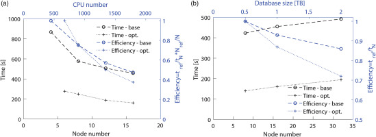
Weak scalability tests have been performed by increasing the number of snapshots while maintaining the parameter nDFT constant, following the approach outlined in Rogowski et al. (2024). The results, depicted in Figure 3b, illustrate the running time (in black) and efficiency (in blue). Notably, the running time remains almost constant for both implementations. It is below 10 minutes for the baseline code, and about 3 minutes for the optimized one even as the database size reaches 2TB. The efficiency consistently remains high, above 70% for both implementations, despite the dataset size quadrupling. In this scenario, the Dask implementation results seem to surpass those reported in Rogowski et al. (2024), since they achieved a 64% efficiency while tripling the dataset size.
Results and discussion
To demonstrate the potential of the modal decomposition framework for loss analysis, the HPDA code is applied to LES of a typically aft-loaded LPT blade. The simulation was conducted using the commercial software STAR-CCM+ and involving a segregated flow model with bounded-central differencing. A 2nd order implicit backward differentiation scheme has been adopted for the time derivative, while the WALE model was selected for the subgrid-scale model. Given the low Mach number (<0.05) of the selected condition, simulations have been run considering an incompressible flow regime, while Reynolds number has been set to 1.1×10⁵. The LPT blades were situated within a stage-like environment, composed of a 2D repeating stage with a degree of reaction equal to 0.5 and the Reynolds number based on the axial chord and exit velocity is 1.1∗105. The computational grid used for the calculations is a 2D-extruded polyhedral mesh, extending for approximately a 25% of the axial chord in the span-wise direction and comprising around 30 million spatial points, with y+<1 and x+=z+≈20 all over the blade profile. More details about the LES numerical setup can be found in Russo et al. (2024). Instantaneous data are collected for a total of 4 blade passing periods, corresponding to a total of 560 snapshots. The HPDA application focuses on the vane blade domain. The first step in the procedure, as described in Biassoni et al. (2024), includes data interpolation from the unstructured mesh to a structured one, which is made as uniform as possible to exclude the volumes in the mode computations. Please also note that this dataset is smaller and different than the one used for scalability tests.
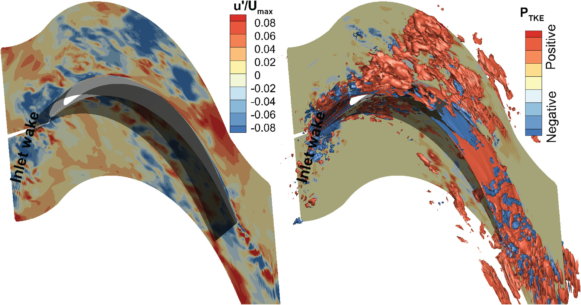
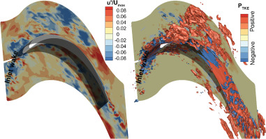
Figure 4 displays the contour plot of the fluctuating axial velocity u′ for a representative snapshot of the instantaneous flow field (on the left). The wake generated by the upstream blade is visible in the snapshot, marked as blue patterns at the domain’s inlet. Each snapshot contributes to the time mean PTKE defined in Equation 2. It is therefore possible to define the quota of PTKE for the kth snapshot at time (tk) as PTKE(tk)=−ρui(tk)′uj(tk)′∂ui¯∂xj. This instantaneous PTKE is shown as a contour plot with superimposed iso-surfaces at low and high production on the right of the picture. Intuitively, it is possible to associate the production of TKE with the inlet wake in the middle of the blade passage. Similarly, positive PTKE occurs in the boundary layer, where back-scatter (conversion of turbulence to mean kinetic energy) is also observed with negative value of PTKE. However, it is difficult to decouple the dynamical features by this approach. Namely, the volume integral of the instantaneous PTKE may only allow the identification of where losses occur.
Figure 4.
Exemplary time snapshot of the instantaneous flow field (left) and instantaneous PTKE (right).
Modal decomposition
The modal decomposition framework aims to overcome the limitation observed in the analysis of the instantaneous flow field. To this purpose POD and SPOD have been already applied to better understand the flow field in LPT (see for example Lengani et al., 2022; Fiore et al., 2023, respectively). However, at least to the best of the authors’ knowledge, the two decomposition techniques have not been directly compared in the turbomachinery research field. Figure 5 aims at summarizing their different properties. Figure 5a shows the relationship between the mode number and the frequency. For SPOD this relationship is about linear since the SPOD modes are obtained at a fixed frequency index as discussed in the section Python SPOD procedure. In this case, we considered Nb=5 and ordered the SPOD modes by frequency index. Consequently, the 5 SPOD modes at the 0 frequency index range from 1 to 5, modes 6 to 10 are at the frequency index 1, and so forth. In contrast, POD modes are orthogonal in time and do not have a fixed or ordered frequency index. The DFT of the POD temporal coefficients may reveal the main frequency of the mode, represented by the black dots in Figure 5a. However, almost all POD modes exhibit more than one active frequency (these active frequencies are depicted by the gray contour). Please note that the inclination of the frequency fit of POD temporal coefficients (dotted blue line) is half of that of SPOD since the SPOD modes are complex-valued and symmetric above the Nyquist frequency. As indicated by Equation 5, each mode carries a portion of the PTKE. The volume integral of PTKE per mode is depicted for the first 15 modes in Figure 5b. Since only nDFT/2+1 SPOD modes were computed (as shown in Figure 1), their magnitudes were doubled to account for their symmetric part (above the Nyquist frequency). Both modal decomposition approaches highlight modes that alone capture more than 1% of the total integral value. Particularly, POD modes 1 and 2, being the most energetic, together capture more than 5%. Similarly, SPOD mode 6, representing the most energetic mode at frequency index 1, captures about 5% of the PTKE. According to Figure 5a, POD modes 1 and 2 and SPOD mode 6 have almost the same frequency, or at least, given the lower frequency resolution of SPOD, they fall within the same frequency bin. Furthermore, POD modes are solely ordered by energy, and, likewise, the PTKE per mode decreases as the mode number increases. However, they may represent considerably different dynamics. For instance, the frequency of POD modes 3 and 4 is much lower than that of mode 5. In contrast, the SPOD modes clearly highlight the frequency band of interest that groups them (as also indicated by the abscissa at the top of Figure 5b).
Figure 5.
Modal decomposition results and comparison between POD and SPOD. The SPOD modes are arranged in descending order of energy, i.e. the first mode at a given frequency is the most energetic. (a) Frequency-mode relationship and (b) Integral value of PTKE per mode.
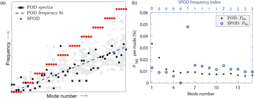
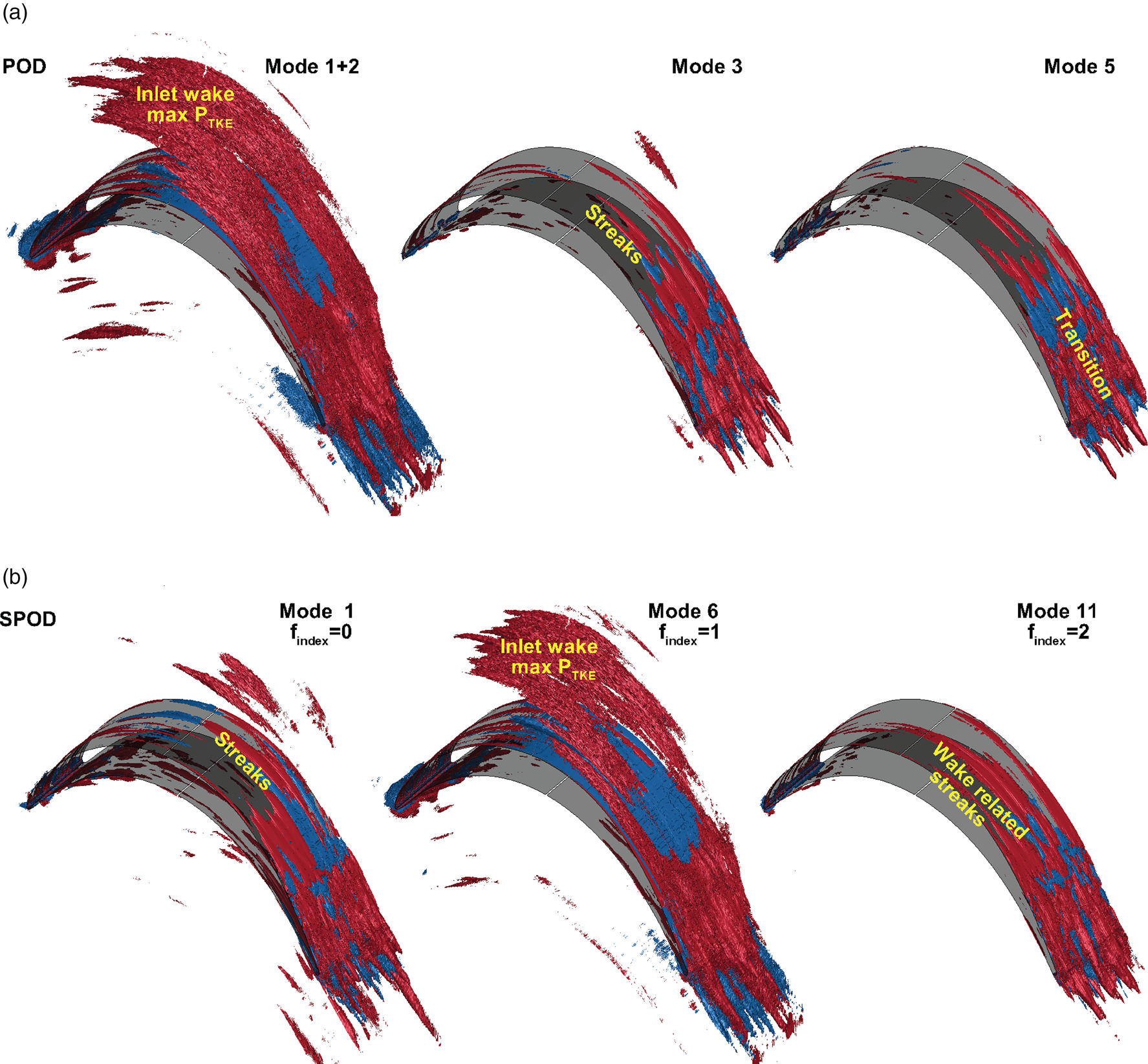
Figure 6a and 6b show the local PTKE for selected modes of POD and SPOD, respectively. To be consistent with the above discussion, POD modes 1 and 2, which represent the periodic deterministic disturbance of the inlet wake (as discussed in Lengani et al., 2019), are summed up. This is consistent with the SPOD representation of mode 6 (the most energetic at frequency index 1), since the SPOD mode is complex and its symmetric DFT part is considered by doubling the real-valued PTKE. The region of maximum PTKE is located within the blade passage, where the highest interaction between the deterministic velocity fluctuations of the inlet wake and the strain within the blade passage occurs. This region is highlighted in yellow in the plots of POD modes 1+2 and SPOD mode 6. Although both representations are quite similar, POD is energetically optimal as it captures larger iso-surfaces. This may be also related to an earlier convergence of POD with respect to SPOD.
Figure 6.
POD (a) and SPOD (b) mode decomposition, PTKE per mode, red and blue iso-surfaces identify regions of production and backscatter, respectively. The most energetic SPOD modes for each frequency index are shown.
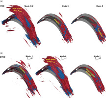
POD modes 3 and 5 capture structures close to the SPOD frequency index 0 and 2 (according to Figure 5a). Namely, the representation of SPOD mode 1 at 0 frequency index is close to POD mode 3, since both track low-frequency streaks (marked in yellow) in the fore part of the blade. This is not the case for SPOD mode 11 at frequency index 2. POD mode 5, in fact, highlights structures related to transition (as marked over the plot) since the iso-surfaces of PTKE appear small and their production (red contour) is limited to the rear part of the suction side (see also Lengani et al., 2022). On the other hand, SPOD mode number 11 at frequency index 2 still highlights a streamwise elongated area of high PTKE, being representative of streaky structures related to the inlet wake perturbations.
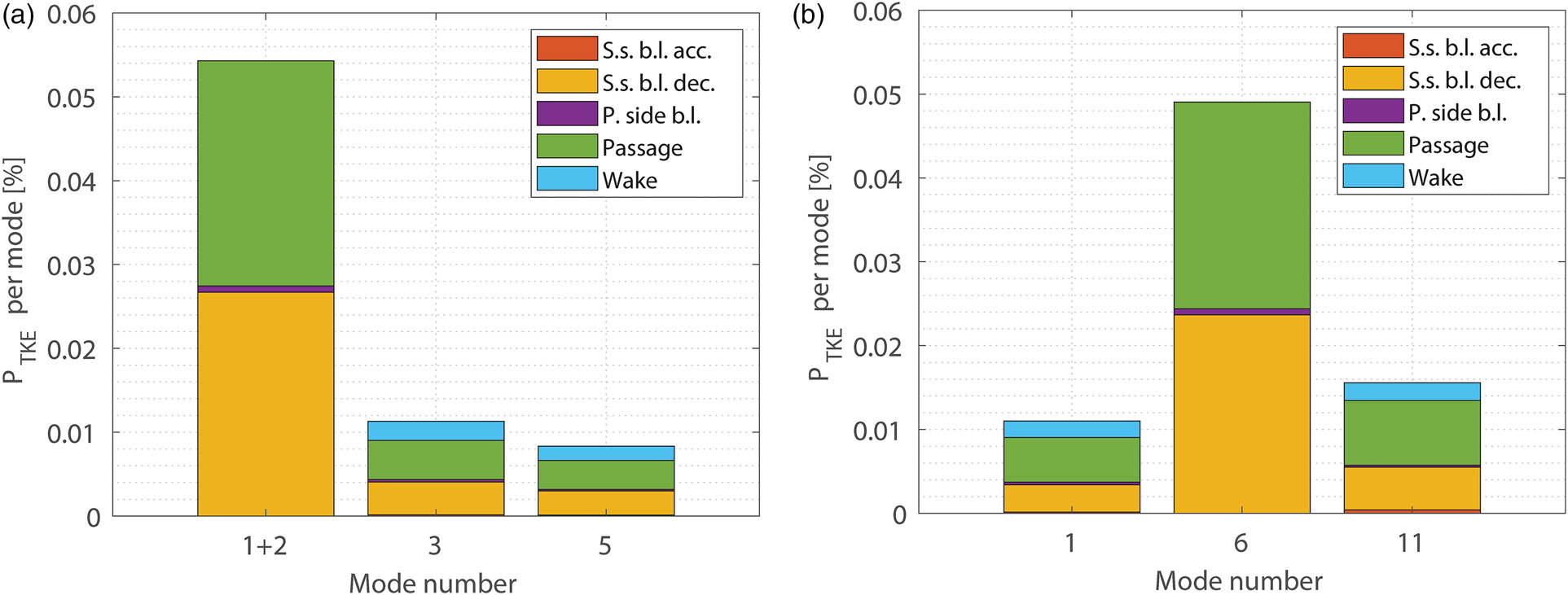
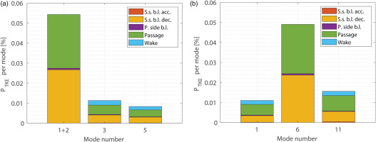
The observations above are confirmed and quantified by the bar charts of Figure 7, where the contribution of the modes under examination to the total PTKE is reported as a fraction for each subregion of interest within the computational domain. This is done by leveraging the properties of the volume integral approach, by which 5 different integration regions are defined: the accelerating part of the suction side in red, its decelerating part in yellow, the pressure side in purple, the wake region (downstream of the trailing edge) in light blue and the passage region in green.
Figure 7.
Bar charts of mode contribution to PTKE per domain zone: POD results (a), SPOD (b).
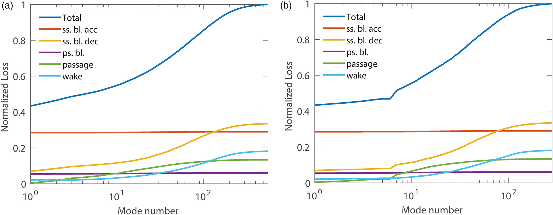
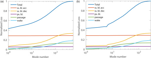
Overall results, as previously discussed in Lengani et al. (2019) and Dellacasagrande et al. (2023), are summarized with the contribution per mode of the volume integral of PTKE (see Equation 5). Figure 8 shows the cumulative loss contribution per mode of POD and SPOD (left and right, respectively). The total loss is depicted in blue. Both modal decompositions lead to the same final integral value and the accuracy of the proposed methodology is within 3% of the inlet to outlet loss computation (see Biassoni et al., 2024). Note that the viscous dissipation is a reference value taken as mode 0. The main difference between POD (Figure 8a) and SPOD (Figure 8b) lies in the distribution of loss with respect to mode number. SPOD makes clear that low frequency content (first 5 modes) has a minor contribution only in the passage region. Otherwise, loss generation in the decelerating part of the suction side and in the wake region is triggered by higher frequency content. It is interesting to note that SPOD representation is almost as optimal as POD while in this latter case the frequency contents are somewhat mixed.
Figure 8.
Cumulative contribution of modes to the overall losses: POD results (a), SPOD (b).
Conclusion
The paper provides an open-access HPDA code for the analysis of the transport equation of total pressure in high-fidelity simulations of turbomachinery. The algorithm of the procedure and its implementation, utilizing Python and the Dask library, are discussed in detail. Strong and weak scalability tests are provided and compared with similar codes in the literature. The current procedure exhibits less efficiency in terms of strong scalability. However, it demonstrates highly efficient weak scalability, making it well-suited for handling very large datasets with low programming effort.
The HPDA code is applied to LES of a typical aft-loaded LPT blade. POD optimally captures (from a mathematical perspective) flow structures and ranks them by energy and, therefore, by PTKE. Conversely, SPOD ranks them by frequency, facilitating the grouping of dynamic features based on frequency bands. Considering the rapid execution time of the current code on large databases, it holds promise for analyzing the growing volume of high-fidelity simulations within the turbomachinery domain. This could lead to achieving an optimal identification of loss sources by pinpointing the dynamic features responsible for these losses.