
Introduction
Extending the operational window is one of the main challenges in gas turbine development as operational flexibility is a key attribute to meet the requirements of tomorrow. Load decrease is limited by a sharp rise in CO-emissions caused by critically low flame temperature. The objective of this work is a CFD-based model, which is able to predict CO in combustion systems operating at part-load conditions. The model supports the development of combustion systems fulfilling future emissions legislations.
Standard combustion models typically face issues predicting CO-emissions in gas turbine combustors. For example, the popular Flamelet Generated Manifold (FGM) model is based on the assumption, that a turbulent flame brush can be described by a set of laminar flamelets. A flamelet is a thin reaction zone dividing unburnt and burnt material. In flamelets, the late CO-oxidation is strongly increased due to the availability of a stable pool of radicals. In contradiction to the flamelet assumption, part-load combustion in gas turbines shows superequilibrium CO in the exhaust gas far behind the heat release zone. It is obvious that the source terms responsible for the burn out of CO cannot be described by flamelets.
Nevertheless, the prediction of CO using FGM can be found in Goldin et al. (2012). Here, the authors used a combination of FGM and a turbulent flame speed model to close the reaction progress source term. The author concludes that FGM drastically overestimates the source terms of CO-oxidation.
Another approach can be found in Wegner et al. (2011). Here, CO is described by its own transport equation. Within the turbulent flame brush, CO is set to the maximum value of CO at a predefined reaction progress state. The peak value of CO is determined by flamelet calculations. The source term describing the CO-burnout is closed by detailed chemistry.
On the basis of literature review, industrial requirements and fundamental studies, we identified the following key elements for our approach:
Turbulence: Due to the technical relevance of this work, we focus on efficient models in order to ensure applicability for industrial applications. Hence, we decided to build the model on the basis of Reynolds-averaged Navier-Stokes (RANS) equations. Note that the presented modeling strategy is not limited to RANS.
Combustion: Simulation of combustors operating at part-load conditions requires advanced strategies in combustion modeling. As the prediction of CO strongly depends on a precise heat release distribution, the FGM Extension model is used (published by the authors in Klarmann et al. (2016)). The advantage of this model is that it is validated on flames which can be characterized by low reactivity. Here, it is inevitable to consider flame stretch and heat loss as it may substantially alter shape and position of the turbulent flame brush. Note that the implementation is able to consider partially premixed combustion. This is of great significance as CO is sensitive to dilution by secondary air.
CO-Model: As already discussed, separating time scales of combustion and late burnout is necessary. As basic studies revealed, the impact of flame stretch and heat loss to CO cannot be neglected. Flame stretch substantially lowers the peak value of CO within the turbulent flame brush. Furthermore, heat loss cannot be neglected as it may substantially decreases the CO-oxidation which is calculated using the temperature dependent Arrhenius law.
Numerical model for CO-emissions
The Favre-averaged transport equation for a generic variable
The terms on the left-hand side (transient term and transport terms) are closed in the context of RANS when considering the generally employed gradient diffusion approach. The Reynolds-Averaged source term on the right-hand side remains unclosed.
This work is using two different approaches to (1) model the combustion by modifying the reaction progress source term closure of FGM
Combustion model: FGM extension
This section is a short summary of the model published by the authors in Klarmann et al. (2016). It is based on the FGM model initially published by van Oijen and de Goey (2002). In the context of FGM, the transport equation for the reaction progress
Here, turbulence is considered by integrating the product of the reaction progress source term and the probability density function P. For the evaluation of P presumed beta-functions are used. This requires additional transport equations for the variance of every control variable (c and f). The model extension modifies the reaction progress source term closure of FGM by a correction factor Γ. The PDF-integrated source term then reads:
Here, Γ is formulated on the basis of flame speeds:
The underlying modeling idea is to divide the unstretched, adiabatic source term
More details on the determination of m can be found in Klarmann et al. (2016).
CO-model
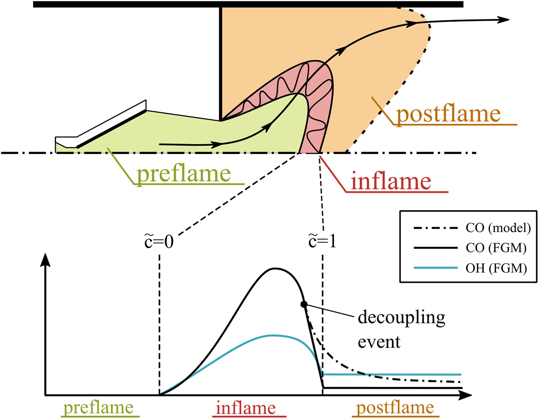
Mass fraction of CO is represented by its own transport equation. Wegner et al. (2011) initially proposed the idea to separate the time scales of CO-burnout from the combustion process. This idea is adopted in this work as we divide the domain in three regions: (1) preflame (inert), (2) inflame and (3) postflame as shown in the upper half of Figure 1. The employed assumption is that CO decouples from the combustion model under specific conditions. This leads to a burnout region behind the turbulent flame brush. Hence, the closure consists of two parts in which CO is treated differently (the preflame region does not require any modeling). Classification in inflame or postflame region is performed by estimating the limiting factor, which can be either turbulence (inflame) or the chemical finite rate of the oxidation of CO (postflame). This is based on the assumption that the inflame situation is dominated by the time scales of turbulent mixing (as chemistry is fast) and the burnout region is dominated by chemical time scales. The lower part of Figure 1 shows the CO-modeling strategy. CO is described to a certain point using FGM. After a decoupling event, CO is described by a burnout model providing substantially lower source terms due to the absence of radicals. All submodels are described in the following sections.
Inflame model for CO
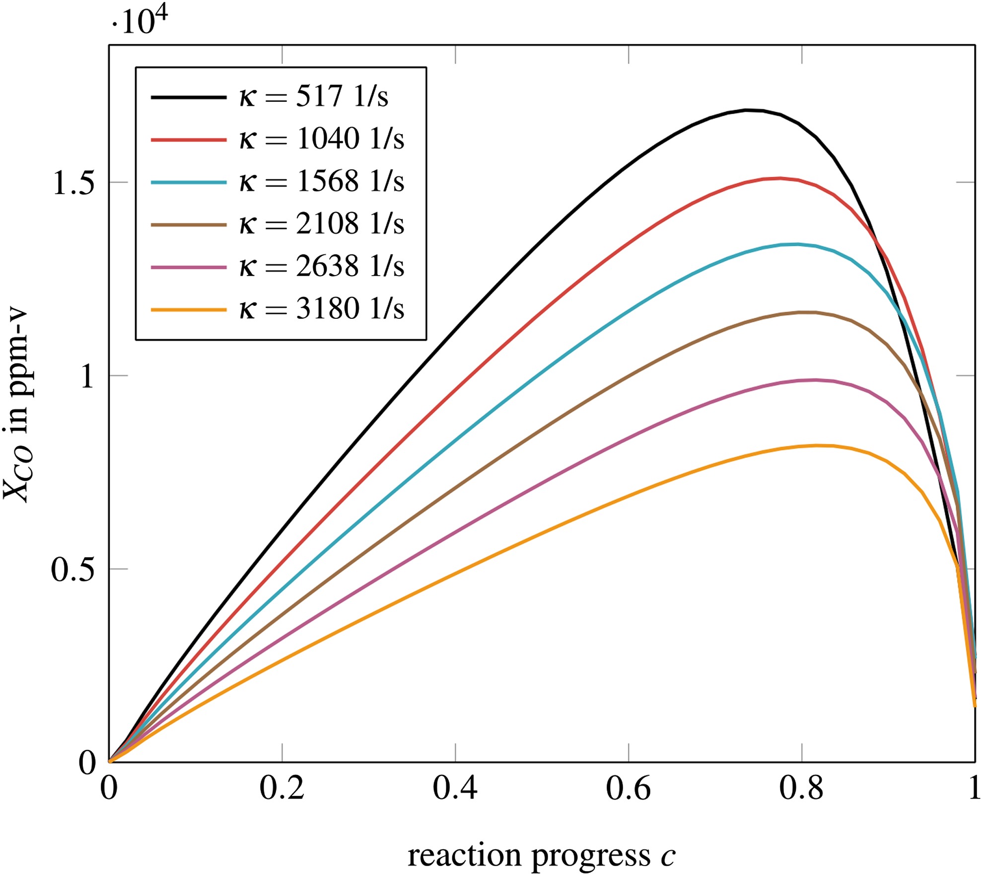
Within the turbulent flame brush, CO-chemistry is fast and interaction with turbulence cannot be neglected. Hence, we tabulate CO on the basis of PDF-integrated profiles of flamelets. CO cannot be accurately represented by flamelets without considering flame stretch and heat loss. Stretch alters diffusion of heat and species which strongly impacts CO. For example, a constant pressure reactor, fully neglecting diffusion, shows significantly higher CO compared to corresponding freely propagating flamelets. Adding the influence of flame stretch using premixed counter flow flamelets steepens the gradients of species and temperature and increases the effect of diffusion. The impact of stretch to CO is illustrated in Figure 2. Note that the impact of heat loss on CO profiles is lower than the impact of flame stretch. Adding stretch and heat loss as additional dimensions to the tabulation process would significantly increase the numerical effort. Therefore, an alternative is presented to model the influence of flame stretch and heat loss. The approach is similar to the correction factor used in the FGM Extension. The tabulation of CO on the basis of unstretched adiabatic flamelets reads:
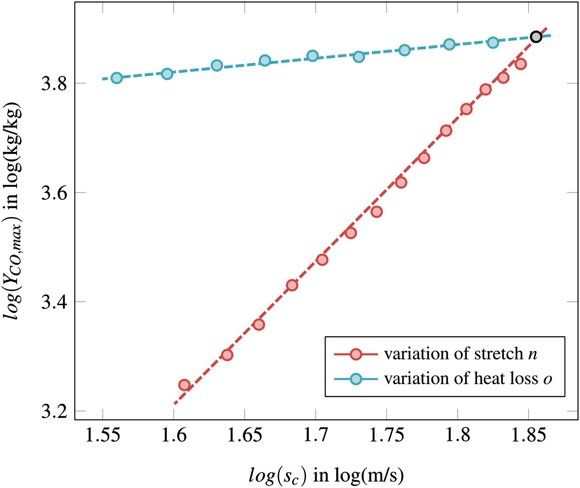
As the proportionality between flame speed and heat loss differs from the proportionality between flame speed and stretch, we introduce two correction factors to consider both effects independently:
This is analytically correct if the following relations are valid:
Direct modeling of these relations is complex. Therefore, we introduce the assumption that the analytical relation is similar to the proportionality between flame speed and the peak value of CO before PDF-integration:
Finally, the proportionality exponents read:
The proportionality exponents are the gradient of a functional correlation between
Postflame model for CO
CO-oxidation in the late burnout (i.e. in the postflame zone) can be described using a single reaction equation:
The proposed CO-model is based on the idea that behind the turbulent flame brush H and OH radicals are in equilibrium. This assumption is based on the fact that the chemical timescales of all radicals are orders of magnitude smaller than these of the CO-burnout. Hence, the postflame source term of CO is calculated using the equilibrium of OH:
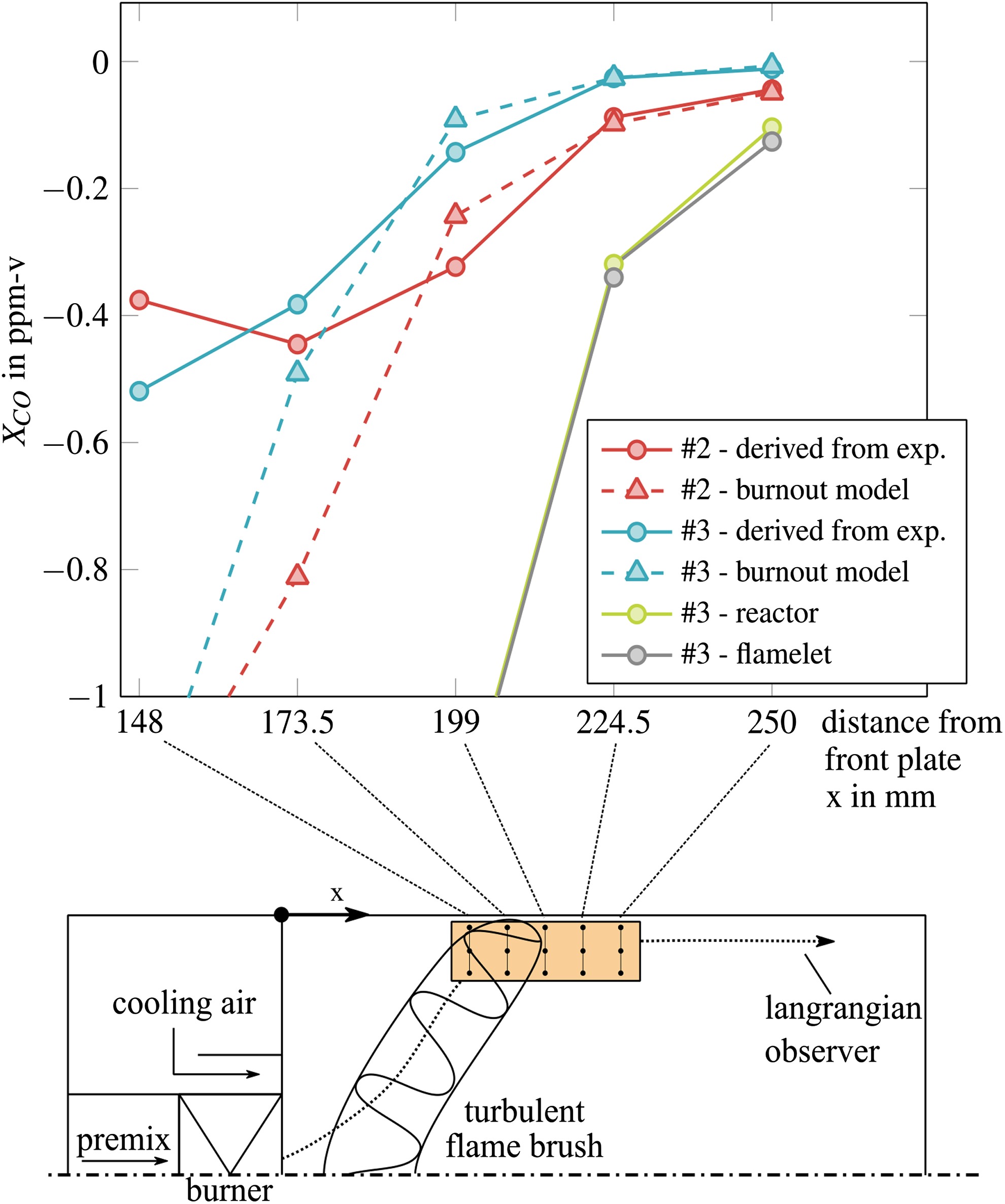
Figure 4 shows the experimental source term for two operating conditions of different adiabatic flame temperatures. Note that the source terms are based on the spatial gradient of CO which can be derived from measurements. The experimental setup can be find the following section. Furthermore, the corresponding source terms calculated by the introduced postflame model is plotted. Downstream of the 199 mm measurement position, the postflame model prediction and the experiments are in good agreement. Furthermore, Figure 4 shows the CO source terms of a freely propagating flamelet and a constant pressure reactor at the corresponding reaction progress (derived from experimentally measured CO2 and CO). As already discussed, they clearly overestimate burnout rates of CO.
Modeling the transition
The Transition model is based on an estimation of the turbulent Damköhler number for CO, which compares turbulent with chemical time scales:
We use the following expression which is the time needed to oxidize CO close to equilibrium:
Multiple definitions for turbulent timescales exist. We decide to use a timescale characterizing eddies of the integral length scale (Poinsot and Veynante, 2005):
This quantity is often used in terms of limiting combustion (e.g. in the Eddy-Break-up hypotheses of Spalding (1971)) as it characterizes the timescale of turbulent mixing.
The decoupling event takes place if
We experienced that this decoupling criterion is robust as there exists a transitional range where the burnout rate of CO for both inflame and postflame model are very close to each other.
Experimental setup
Experiments are conducted in an atmospheric single burner test rig with a thermal power of 50 kW. Details of the burner can be found in Sangl (2011). The setup is depicted in Figure 5. An electrical preheater is providing air at a temperature of 300 °C. Within the burner plenum, air is divided into primary air, which is swirled by the burner, and secondary air. The secondary air is bypassing the burner as it flows through a perforated plate into the combustion chamber. Fuel is injected at the burner slots.
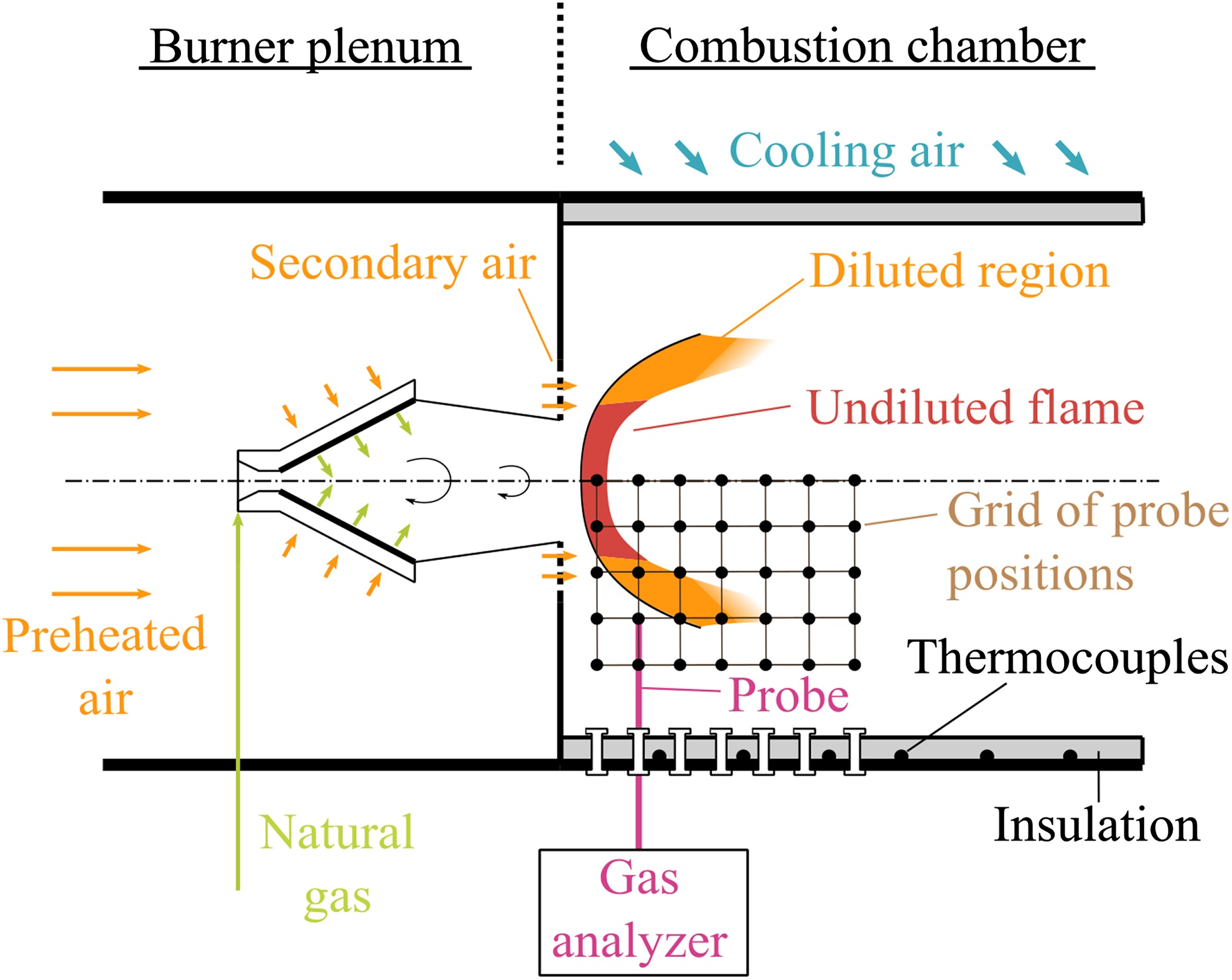
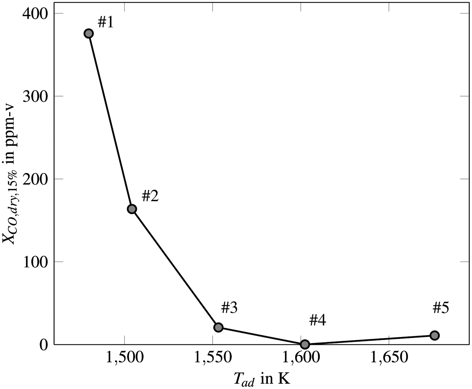
Within the combustion chamber, swirling fuel-air mixture generates a vortex breakdown, where the flame stabilizes at the stagnation point. The outer part of the turbulent flame brush is diluted by secondary air, providing a region of strongly decreased reactivity, leading to elevated CO-emissions. Ceramic insulation prevents significant heat losses, which leads to similar conditions as present in gas turbine combustors. Furthermore, the chamber is cooled by impinging air. Local measurements are conducted using a water-cooled probe, which can be traversed in radial direction. Furthermore, the probe can be attached to multiple ports, which are located at several downstream positions. This enables the measurement of a two-dimensional grid. Note that due to the fact that the combustion chamber is cylindrical, we can assume rotational symmetry. This is advantageous as a two-dimensional grid measurement is sufficient to derive a volumetric distribution. We checked this assumption by comparing multiple CO-profiles over radius of same axial positions. A gas analyzer is used to determine mole fractions of CO2, O2, NOx, CO from the extracted gas samples. In order to evaluate heat loss precisely, temperature is monitored at the outer shell of the insulation using thermocouples. Measurements are conducted at five different adiabatic flame temperatures:
#1-3: Superequilibrium CO.
#4: Transition of incomplete burnout and equilibrium.
#5: CO is in equilibrium.
Figure 6 depicts CO as a function of adiabatic flame temperature. Note, CO is measured at a characteristic residence time of about 20 ms.
Validation
All introduced models are implemented in Fluent (Ansys, 2014) using a C-based interface. Tables are used to provide the required model input during runtime. All table entries are quantities derived from equilibrium calculations as well as premixed counter flow flamelets at predefined stretch rates, enthalpy defects, and mixture fractions. The preprocessing of the tabulated data is performed using a Python-based routine on the basis of the chemical kinetic software Cantera (Goodwin et al., 2015). Around 5,000 flamelet calculations have been used to generate the table. Table 2 lists some information of the CFD setup. Geometry is shown in Figure 7 and boundary conditions are listed in Table 1. The domain is a quarter of the original geometry using periodical boundary conditions. Note that the precise evaluation of wall heat loss is crucial to predict CO-burnout due to its temperature sensitivity. The non-adiabatic boundary condition is evaluated using temperature profiles measured at the outer shell of the insulation. We decided to use transient (URANS) simulations as we experienced unsteadiness using steady-state simulations. All results shown in the following are time averaged from the transient results.
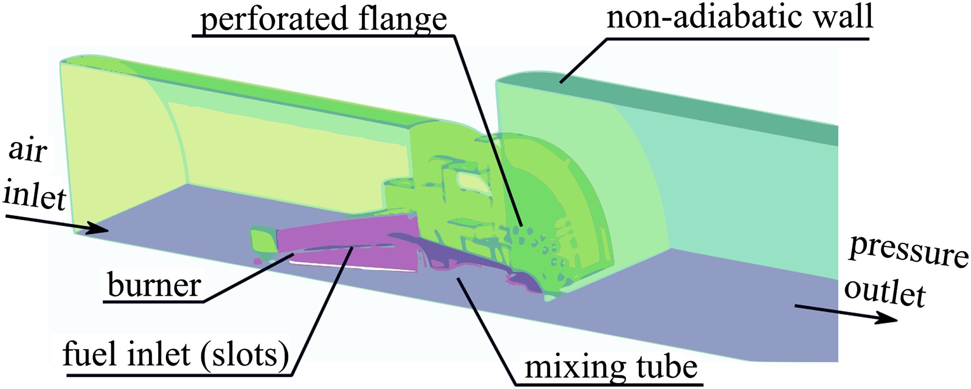
Table 2.
Numerical setup.
| Table Generation | |
| Chemical mechanism | GRI 30 (Smith et al. 2014) |
| Points of mixture fractions | 50 |
| Points of enthalpy defects | 20 |
| Points of strain rates | <15 |
| Prop. exp. reaction progress m | 1.5 |
| Prop. exp. CO stretch n | 2.0 |
| Prop. exp. CO heat loss o | 0.37 |
| CFD | |
| Software | Fluent v15.0 (ANSYS Inc. 2014) |
| Mesh (chamber only) | polyhedral, 2.4e5 cells |
| Sct | 0.7 |
| | 1.0 |
| Periodicity | Quarter |
| Turbulence closure | k- |
| Pressure-velocity coupling | simple |
| Upwind order | second order |
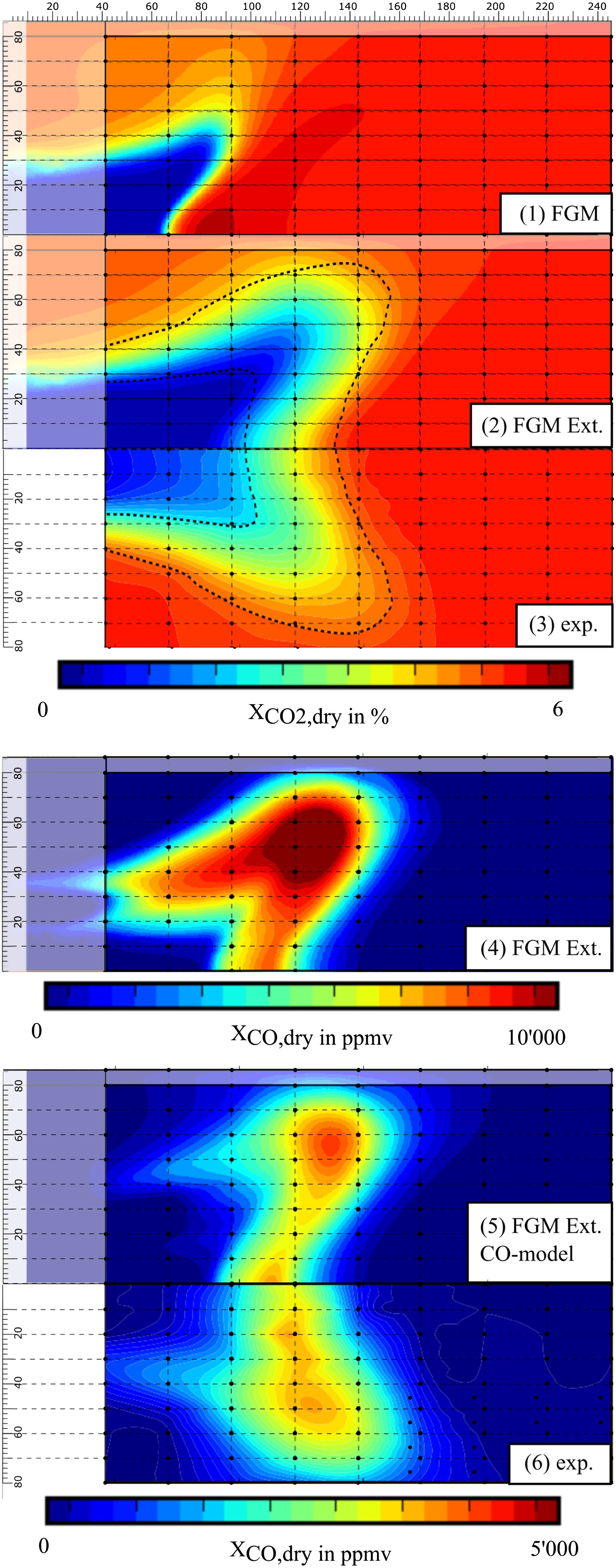
Figure 8 illustrates experimental and numerical contour plots of CO of operating point #4. The heat release distribution (indicated by
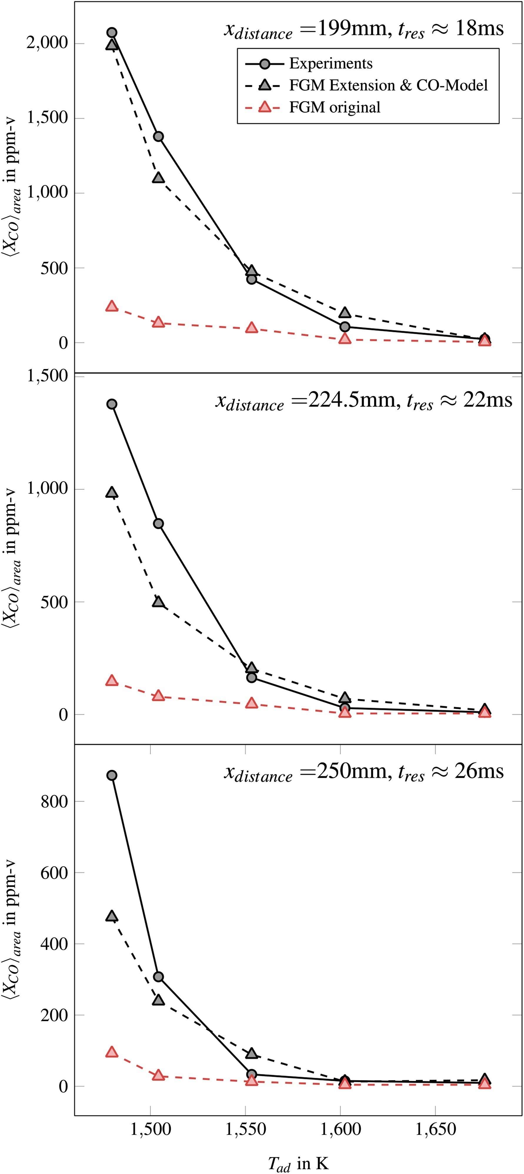
For the purpose of quantitative validation, it is reasonable to compare surface-averaged quantities as a probe position with high radius represents more surface than a position with low radius. Hence, we accumulate the product of CO and its corresponding ring face and divide the product by the total surface:
Figure 9 compares averaged CO values of experiments and simulations at three different axial position:
Summary, conclusions, and outlook
The paper presents an approach to predict CO-emissions numerically. The necessity of modeling CO on the basis of combustion models is discussed. Previous approaches and fundamental studies revealed that timescale separation between fast combustion and slow CO burnout is necessary. Hence, the proposed model is divided in an inflame and a postflame part. As we showed, inflame-CO cannot be described by tabulating freely propagating flamelets as flame stretch plays a major role. A model for the stretch and heat loss dependent correction of CO is presented. Furthermore, the source terms describing the late CO burnout behind the heat release zone is modeled by a single elementary reaction equation. Here, we introduced the model assumption that OH is in equilibrium after it decouples from the turbulent flame brush. This assumption was verified by comparing source terms derived from experiments with source terms calculated by the proposed postflame model.
All models are implemented in a commercial CFD-software and validated against experimental data. The numerically predicted CO agrees well with experimental data for different axial probe positions. Furthermore, we showed the strong underestimation of CO if FGM is used without any further modeling. This underlines the necessity of dedicated CO models to predict elevated CO-emissions.
Validation of high-pressure multi-burner configurations is planned in the future: In part-load operation, only a part of the burners are supplied with fuel. This leads to the situation that hot burners interact with cold air from the inactivated neighbouring burners.
Nomenclature
Latin
A
Area, m2
c
Reaction progress, -
Dat
Turbulent Dammköhler number, -
f
Mixture fraction, -
karr
Reaction rate constant
k
Turbulent kinetic energy, m2/s2
Mass flow of air, kg/s
m
Proportionality exponent for progress source term correction, -
n
Proportionality exponent for stretch correction, -
o
Proportionality exponent for non-adiabatic correction, -
P
Probability density function, -
p
Pressure, Pa
Sc
Turbulent Schmidt Number, -
sc
Fuel consumption speed, m/s
t
Time, s
T
Temperature, K
u
Velocity, m/s
x
Spatial coordinate, m
Xi
Mole fraction of species i, -
Yi
Mass fraction of species i, -