Introduction

The use of vaned diffusers and its assessment to aerodynamic performance is of importance for a centrifugal compressor. Industrial centrifugal compressors are often used in oil and gas applications that necessitate operation over a range of speeds, operating pressures and flows. A stage of compression in a centrifugal compressor comprises of the inlet system, an impeller, a diffuser portion followed by a cross-over and a return vane (in the case of a middle stage of compression) or a volute/scroll (in the case of an exit stage of compression). Diffusers play a key role in static pressure recovery for each stage of compression.

In a centrifugal compressor, the impeller imparts kinetic energy to the gas. The gas exiting the impeller requires conversion of the dynamic enthalpy to static pressure that is usable from a compression standpoint (Ludtke). The diffuser thus performs the role of a pressure recovery device, thereby converting the kinetic energy to usable static pressure rise (Flathers, 1997). Vaned diffusers were originally proposed by Senoo (1978), who had noted that the presence of a throat in the vanes can lead to a loss in usable flow range for the compressor. Subsequently (Senoo et al., 1983), the low solidity diffuser/airfoil (LSD, LSA) was introduced, where the efficiency improvement from the LSDs was noted to be on par with those of vaned diffusers with minimal change to the usable operating flow range when compared to vaneless diffusers. The performance of LSDs in centrifugal compressors has been documented in Sorokes and Welch (1992), Amineni et al. (1996). Multi-rows of diffuser vanes (Sorokes and Kuzdzal, 2010) have been shown to control boundary layer growth and reduce losses in the diffuser passage, while contributing to performance benefits when compared to a single row of vanes.

The aerodynamic design for a vaned diffuser depends on several parameters such as (Grönman et al., 2013) the vane profile shape, vane incidence, radial gap between the impeller exit and the leading edge of the diffuser vane, and solidity (which relates to the vane count, vane turning angle and the vane length). The influence of solidity on the diffuser performance was investigated in detail by Engeda. Low solidity diffusers with solidity in the range of 0.6–0.9 was investigated, and Engeda had demonstrated that it is possible to design LSAs over a range of operating flows and a range of solidity. The vane profile plays a key role in the design process. The use of NACA 65-(10) profiles for the vanes has been noted to maximize the efficiency gain at the design point (Grönman et al., 2013). In centrifugal compressors with modular rotors, the presence of a module center-stud influences the size of the vane thickness, and subsequently the vane profile geometry.

In this paper, the aerodynamic performance characterization of modular-rotor centrifugal compressors with LSAs is presented. The paper is organized as follows: an overview of the design process for LSAs is presented in section 2. This is followed by a single-stage test rig evaluation of the proposed LSAs, and a comparison of test results for the vaneless diffuser versus LSAs is presented. A version of the tested LSA was implemented on a full-scale centrifugal compressor and high pressure test results are presented in section 4.

Exit velocity triangle

The basis for the stage aerodynamic performance calculations and its relationship to Euler's equations can be obtained from the exit velocity triangle. The impeller in a centrifugal compressor imparts kinetic energy to the gas by virtue of rotational velocity. The exit velocity triangle presents a convenient framework to visualize the gas flow exiting the impeller. The methodology presented in this section closely follows the work of Casey and Robinson (2022a,b). We refer to Figure 7 for the station number nomenclature. The vector relationship between the absolute velocity C, the impeller tip speed U and the relative velocity W is given by

where the subscript ₂ denotes the impeller exit (refer Figure 1). The gas exiting the impeller eventually gets channeled into a stationary component. The stationary component following the impeller can be one of two kinds:

Figure 1.

Exit velocity triangle. The insert on the left shows the velocity triangle in relationship to the impeller exit blade angle. The velocity triangles on the right depict the changes to the meridional component as flow is increased across a constant speedline.

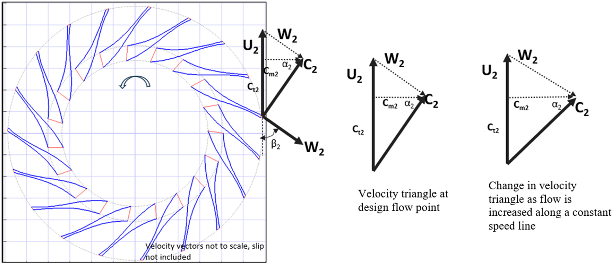
The blade exit angle with respect to the tangential direction is denoted by β2. In a rotating frame of reference, a gas particle exiting the impeller exits with a velocity W2 in the direction aligned with the blade exit angle. The tangential velocity imparted by the blade to the gas particle due to rotation is given by U2=D2Ω, where D2 is the impeller exit or tip diameter and Ω the rotational shaft speed. The absolute velocity C2 is the vector-sum of U2 and W2, as can be noted from Figure 1. The meridional component of the velocity is denoted by Cm2, and the tangential component by Ct2. The meridional velocity component is proportional to the volumetric flow rate through the impeller. For a specified tip speed U2, the meridional velocity increases as flow is increased from the best efficiency flow point to the choke flow point at constant speed. The tangential velocity Ct2 is proportional to the head and enthalpy rise of the impeller as related to the Euler's equation. This is depicted in the velocity triangles shown in the right-hand side of Figure 1. The tangential and meridional velocity terms can be non-dimensionalized with respect to U2 to obtain

Here, λ is the non-dimensional work coefficient, related to the head-rise (and enthalpy rise) across the impeller. While Casey and Robinson (2022a,b) denote this as a flow coefficient, we use the term “normalized flow coefficient” denoted by ϕn2 to avoid confusion with the volumetric flow coefficient (to be introduced in the next section). The velocities normalized to U2 result in the following trigonometric relationships:

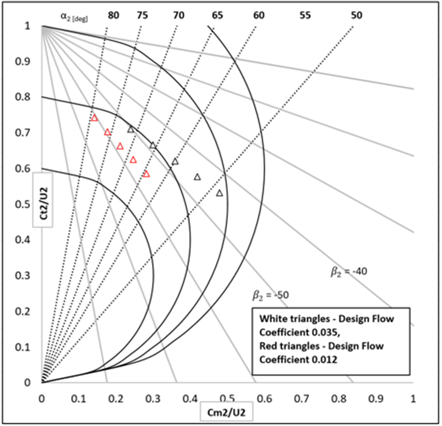
The non-dimensional plot of λ vs ϕn2 presents a convenient framework to clearly visualize changes to flow and its relationship to the exit blade angle from a 1D standpoint. Lines of constant flow angles α2 are denoted by straight lines starting from the origin at the bottom left corner of the plot. Lines of constant reaction ratios are denoted by circles passing through the origin. Diagonal lines originating at (0,1) indicate lines of constant blade angle β2.

A plot of λ vs ϕn2 is shown in Figure 2 with design data overlaid for two different staging selections within an impeller family. Of importance is the use of the plot as a design tool to set the impeller exit angle, and to visualize the changes to the design as a function of the discharge flow coefficient. The diagonal lines representing the flow angles α2 can be used to compare against stall criteria such as Senoo's criteria (Fulton and Blair, 1995). From a practical engineer's standpoint, this plot closely resembles a head-flow plot and thereby provides useful guidance from an aerodynamic design perspective. And more importantly, the plot can be used to set a stagger angle for the LSA vanes prior to start of a more detailed CFD analysis.

Figure 2.

λ vs ϕn2 plot with design data for ϕ=0.012 and 0.035.

General layout

The general layout of the diffuser is a parallel wall diffuser with vanes, guiding the flow into a volute. In the case studies presented below, the baseline configuration only uses vanes at the outer diameter (referred to here as exit guide vanes, EGVs), while the LSA's are added at the inner diameter (see Figure 5 for details).

Design considerations for LSAs

The design flow coefficient for an impeller is denoted by the inlet flow Q to the stage. We denote this coefficient as ϕ, and it is non-dimensionalized using the rotor speed N [rpm], Q [cfm], D2 [in] as follows:

ϕ=700.3QND23

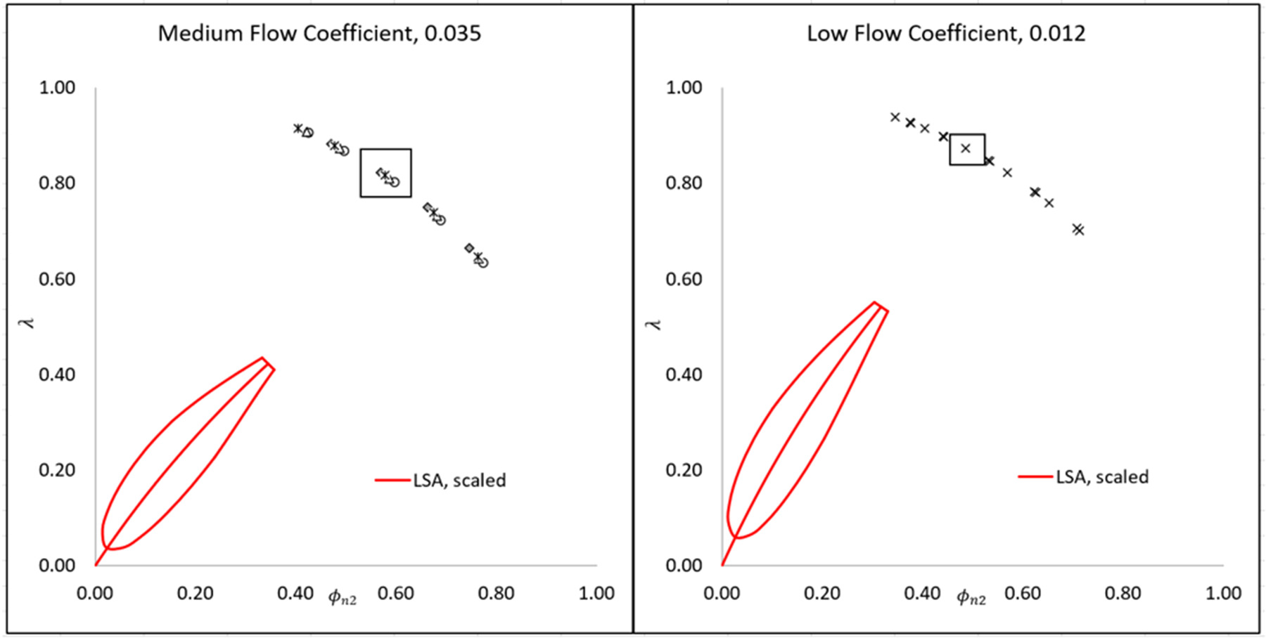
In the current work, low solidity airfoil diffuser designs are presented for two impeller stages with design flow coefficients of 0.035 (medium flow coefficient) & 0.012 (low flow coefficient). The representation of both these designs on a λ vs ϕn2 plot is shown in Figure 3. The plot shows the predicted performance characteristics obtained from CFD (represented by the symbols). The best efficiency point is highlighted, along with the performance predictions over a range of inlet flows. Also overlaid on the plot is the scaled insert of the LSA depicting the airfoil shape under consideration. The stagger angle of the LSA was determined in each case to meet the intent of the design flow condition. The λ vs ϕn2 plot therefore helps to provide a first pass estimate at the stagger angle for LSA design.

Figure 3.

Non-dimensionalized λ vs ϕn2 plot with stagger angle depicted for the LSA design, and the boxed point depicting the design flow condition. Data points shown were obtained from CFD.

CFD analysis

A steady-state CFD analysis was performed to assess the performance of LSAs and to design the shape of the airfoils. Several key considerations influencing the stage performance were accounted for during the design, some of which are outlined below:

• - location of the vane leading edge with respect to the impeller (i.e., radius ratio)

• - influence of vane solidity on stage performance

Solidity σ of diffuser vanes is defined as (Engeda)

σ2=(RTE/RLE)2+1−2(RTE/RLE)cos(βTE−βLE)2−2cos(360/Z)

where RLE,RTE are the LSD vane leading and trailing edge radii, βLE,βTE are the blade angles at the leading and trailing edge of the LSA and Z the LSA vane count.

The location of the vane's leading edge in relation to the impeller exit is an important consideration. From an aerodynamic perspective, positioning the leading edge of the vane in close proximity to the impeller exit helps maximize the static pressure recovery in the diffuser. However, the effects of rotor-stator interaction need to also be taken into consideration in this regard. Positioning of the vanes close to the impeller has also been noted to result in increased noise and vibrations (Grönman et al., 2013). A radius ratio (i.e., ratio of LSA leading edge radius to impeller tip radius) of 1.1–1.2 has been noted to be a good choice for design. The current work uses a 1.2 radius ratio.

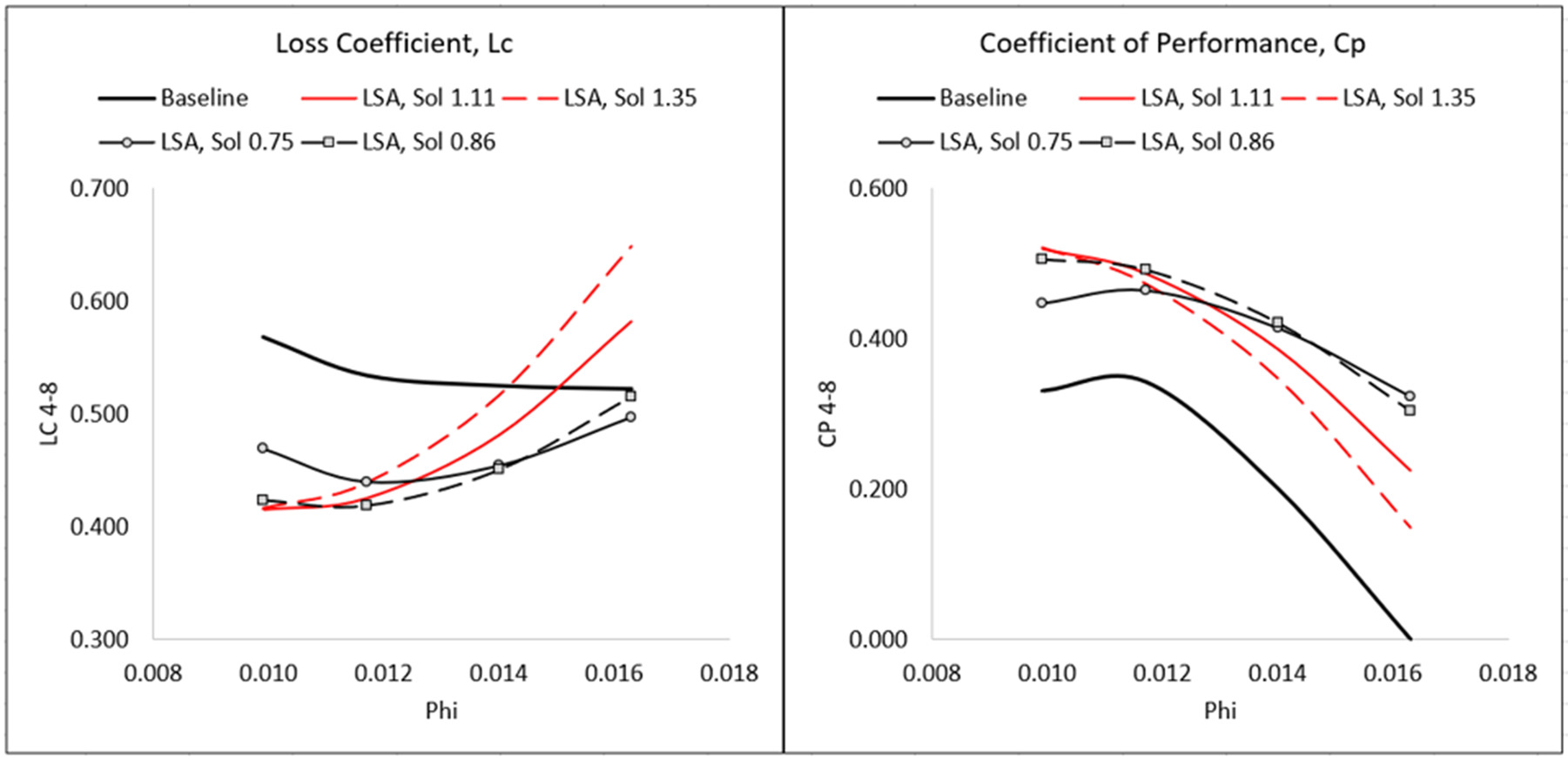
The primary aim of the LSA in this current work was to achieve the same design point efficiency compared to the baseline, with minimal reduction to the operating flow range. The diffuser's ability for pressure recovery was assessed in each design iteration by evaluating the loss coefficient (LC48) from station 4 (located at the entrance to the vertical diffuser after the pinch) to station 8 (at the exit of the volute), and the coefficient of performance CP48. These quantities are defined as follows:

LC48=Pt4−Pt8Pt4−Ps4,CP48=Ps8−Ps4Pt4−Ps4

The final LSA design was chosen based on assessing these parameters, and chosen to maximize the coefficient of performance (i.e., minimize the loss coefficient). The influence of vane solidity on the loss coefficient and coefficient of performance is shown in Figure 4. Based on the CFD results, a solidity of 0.86 was chosen to maximize the static pressure recovery in the diffuser.

Figure 4.

Lc and CP versus flow coefficient comparison for LSA designs; Sol refers to the solidity.

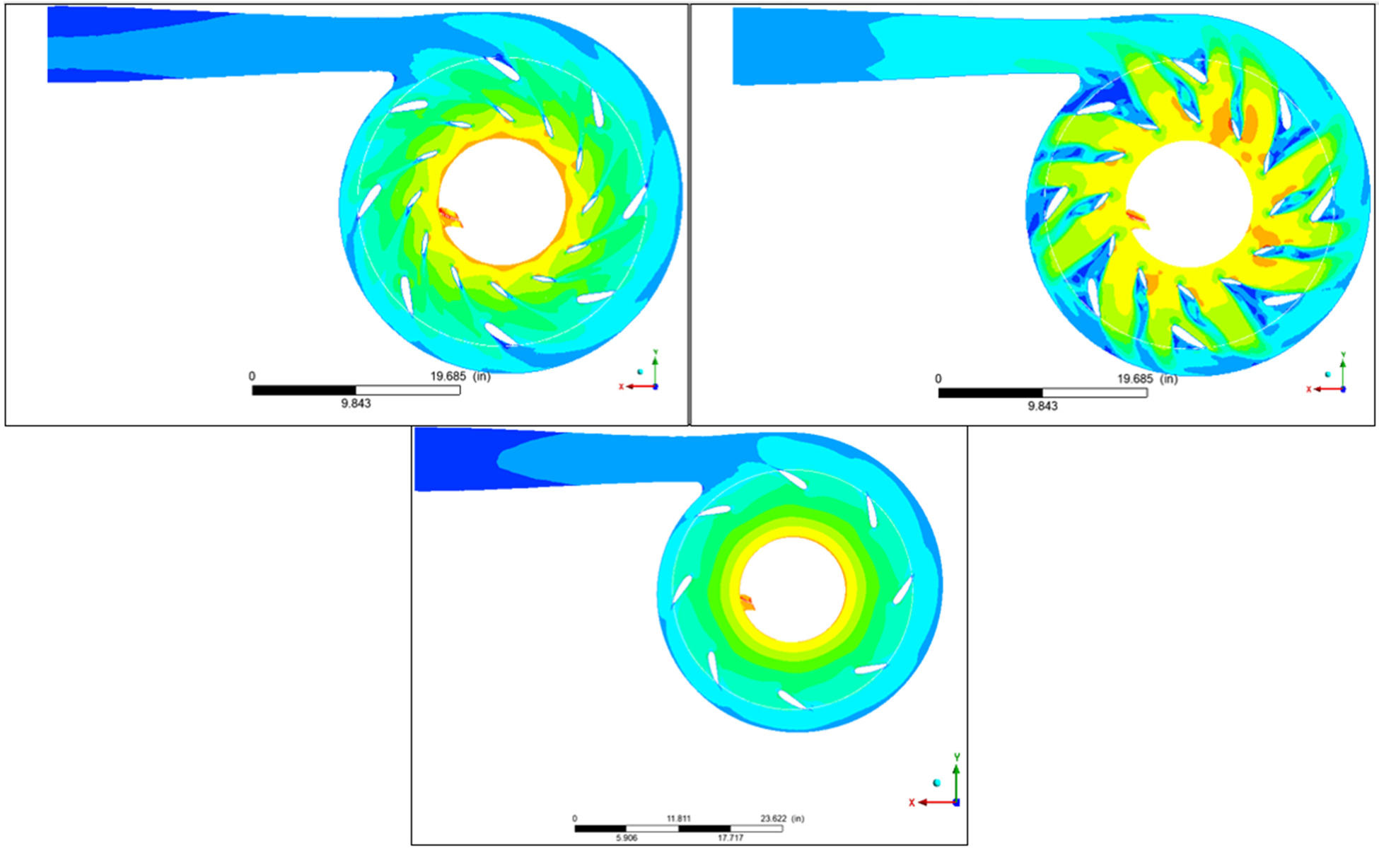
A steady state CFD analysis was performed with the impeller, diffuser and volute domains. The simulations were performed in CFD at a machine Mach number of 0.60, with air treated as ideal gas as the medium. The diffuser domain consisted of two rows of vanes (LSAs and EGVs) as shown in Figure 5. The steady state analysis was performed using a Reynolds Averaged Navier Stokes (RANS) shear stress transport (SST) turbulence model. The impeller was set to a rotating domain, with mixing plane interface between the impeller and diffuser domains. A single passage geometry was used for the impeller domain, while 360-degree models were implemented for the diffuser and volute domains to address the non-axisymmetric flow field. The Mach number contours are shown in Figure 5, where the contours are compared at the design flow point (left) versus maximum flow point (right) at the same speed. It can be observed that as the flow condition is increased towards choke, the separation from the vanes increase the aerodynamic blockage in the diffuser flow path, thereby resulting in increased diffuser losses (and reduced pressure recovery). In contrast, the flow contours at the design point show no separation or aerodynamic blockages downstream of the LSAs.

Figure 5.

Mach number contours with two rows of vanes (first row of LSA vanes); top-left – design flow point; top-right – maximum flow condition; bottom – baseline configuration.

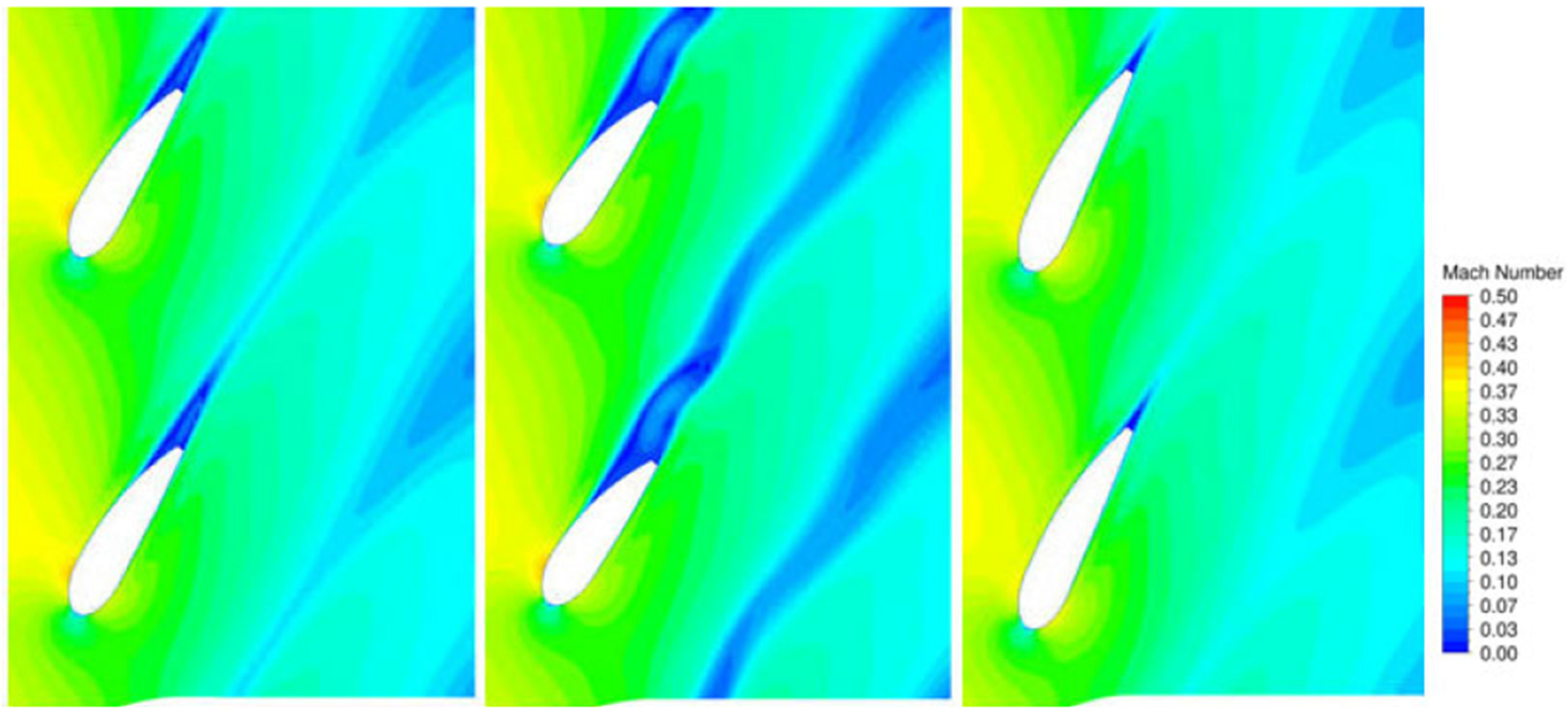
The influence of the vane stagger angle at the design flow point is shown in Figure 6. The contours have been plotted at a 50% streamwise span between hub and shroud for the LSA. The vane stagger angle was set based on the minimizing flow separation downstream of the vanes and taking into consideration the entire operating range of flows. The plot shows the vane stagger angle varied parametrically from β2=45∘ to 55∘. The vane angle was set based on considerations for not only the design flow point, but with the entire flow range of operation.

Figure 6.

Influence of vane stagger angle on Mach number contour; left – exit blade angle 50 deg, middle – 45 deg, right – 55 deg. The influence of the wake at the vane trailing edge as a function of the vane stagger angle can be noted from the above plot.

Single stage scaled testing

The optimized LSA design presented in the prior section was tested in a single stage centrifugal compressor test rig at the OEM's Aerodynamic Test Facility. A detailed description of the test facility can be found in Marechale et al. (2015). An overview of the test setup, instrumentation and sequence of tests is presented here. The closed-loop test setup houses an experimental test rig with a stage of centrifugal compression driven by a 200 HP [149 kW] motor coupled via a speed-increasing gearbox (ratio of 1:9.27). A schematic of the facility is shown in Figure 7. The test rotor is capable of operation up to a speed of 21,860 rpm. Air is used as the test medium, with suction pressures up to 85 psia [5.9 bara]. A venturi is used for flow measurement, and the flow is controlled using three throttle valves downstream of the compressor exit, as shown in Figure 7. Insulating jackets are provided around the test rig piping to maintain an adiabatic compression process and to obtain accurate temperature measurements. The downstream throttle valves are used to control the pressure ratio, and the inlet temperature is controlled by adjusting the water flow rate to the heat exchanger.

Figure 7.

Scaled test rig loop schematic (left) and cross-section (right). Boxed-red numbers depict station number nomenclature.

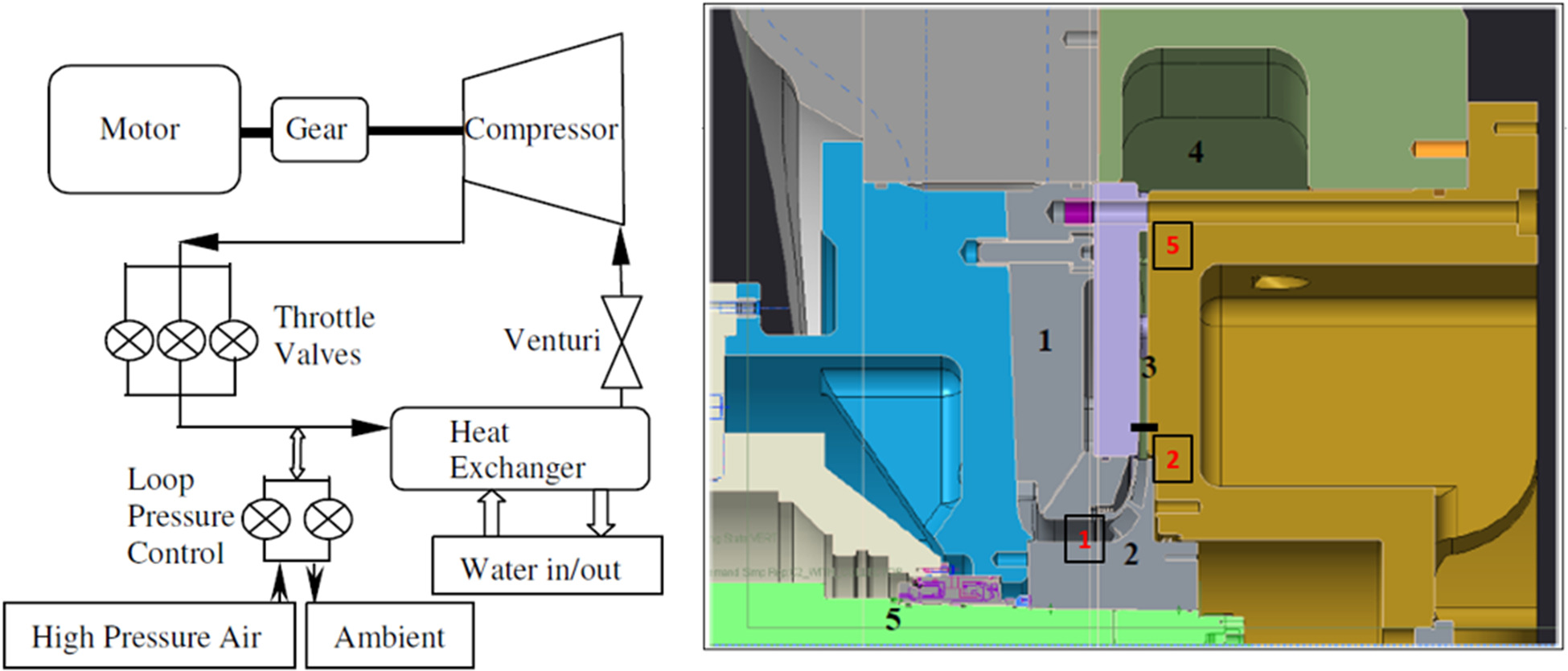
A cross-section of the flow path components for the stage of compression in the scaled test rig are shown in Figure 7. These include an inlet guide vane (labeled as 1), impeller with a front shroud (2) and a parallel wall diffuser with an exit guide vane (3). The horizontal black line in component 3 of Figure 7 shows the location of station 4, where the LSAs were positioned during the test. The test rig is equipped to run as a single-stage compressor with a discharge volute (to model an exit- stage arrangement in a centrifugal compressor) or with a return vane (to model an intermediate stage of compression). The arrangement shown in Figure 7 depicts the exit-stage arrangement with a volute. The collection region at the entrance to the volute is denoted by label 4. The stub shaft and the gas seal components that house the impeller are depicted by label 5.

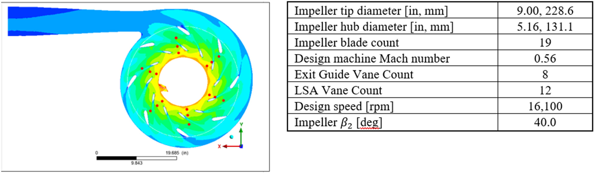
Testing was performed at three different speeds for the baseline case with single row of vaned diffusers at the entrance to the volute. Due to the positioning of the vanes, we refer to these as exit guide vanes. The results were then compared with a second row of LSA vanes positioned downstream of the impeller (in addition to the exit guide vanes). The details of the rig components are noted in the table in Figure 8. The total-to-total stage performance was measured using Kiel probes and thermocouples at the suction and discharge ends. Static pressure taps were instrumented in the diffuser, both upstream and downstream of the LSA. The locations of the static pressure taps (as observed from the inboard side of the test rig, i.e., the left side in Figure 7) are shown in Figure 8, denoted by the red circular symbols. The static pressure taps were spaced 60-degrees apart at three radii locations, corresponding to upstream of the LSA, downstream of LSA and upstream of the exit guide vane.

Figure 8.

Locations of static pressure taps (shown as red shaded circles) in the scaled test rig.

Scaled test results

Figures 9 and 10 shows the static pressure ratio measurements collected from the test rig. Also shown here are the predictions from CFD calculations. At Station 4 (located upstream of the LSA, and downstream of the diffuser pinch), the circumferential pressure distortion arises due to the flow separation from the LSAs. This is evident from the 12 peaks (Figure 9, right) in CFD, corresponding to the 12-vaned LSA. Downstream of the LSA, the flow distortion is governed by the EGV. That explains the 8 peaks from the 8-vaned EGV at Station 5.

Figure 9.

Static pressure ratio at Station 4 to inlet; left – one row of EGV vanes; right – case with LSAs and EGVs.

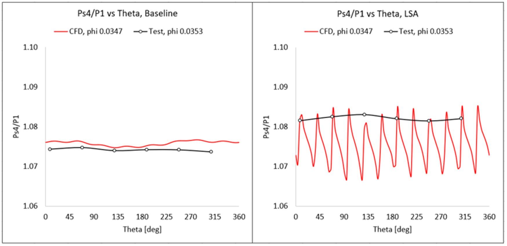
Figure 10.

Static pressure ratio at Station 5 to inlet; left – one row of EGV vanes; right – case with LSAs and EGVs.

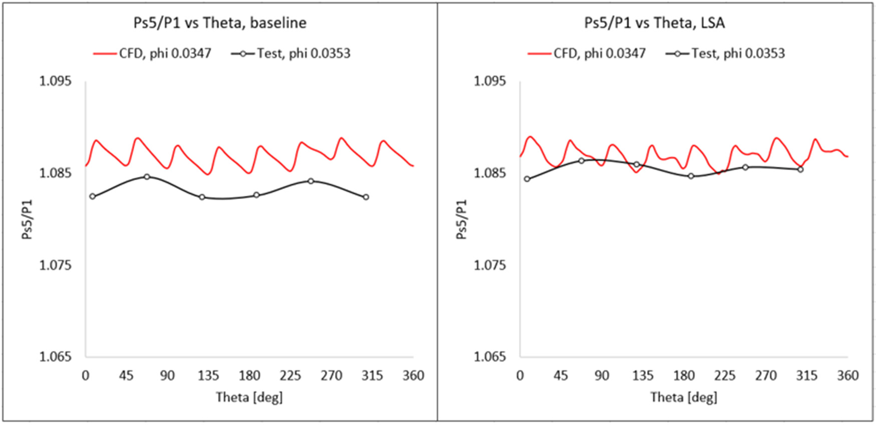
The peaks (on the plot below) can be explained by the flow separation arising from the LSAs in the diffuser. It is relatively straight-forward to plot the full 360-list of profile points from CFD. For the test rig, however, we only have 6 static pressure taps circumferentially located every 60 degrees. Even with the limited measurements for static pressures, we are able to see the correlation between CFD and test, and help validate the CFD results.

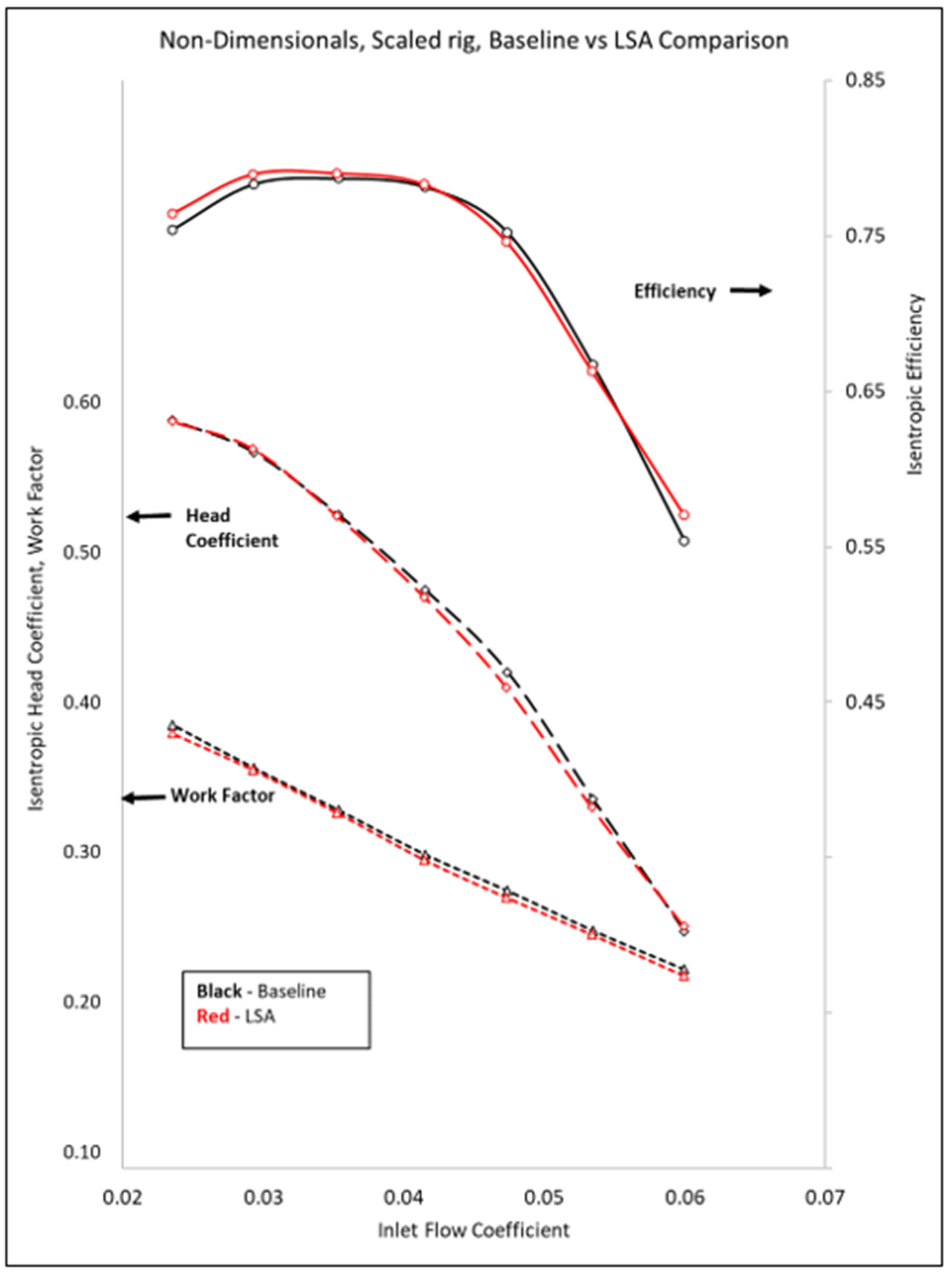
The non-dimensional performance characteristics for the two tested flow coefficients are shown in Figure 11. As noted earlier, the primary aim of the LSAs was to ensure a minimal reduction in the operating flow range, and minimize any impact to performance on the high flow side of the map. The scaled test results show that the LSAs achieved the intended performance.

Figure 11.

Non-dimensional performance, scaled test rig.

Full-scale compressor testing

Full-scale testing was conducted on an inline 6-stage centrifugal compressor operating at a design inlet flow coefficient of 0.03. The testing was performed at the OEM's closed loop test facility. A schematic of the test loop is shown in Figure 12. The facility is capable of closed loop test on air, nitrogen, carbon dioxide and natural gas. The safety relief valve for the discharge pressure is set at 5,000 psia [345 bara]. The compressor was driven by a 15 MW class 2-shaft gas turbine via a speed-increasing gearbox with a ratio 1:1.8. The inlet gas volumetric flow to the compressor was monitored using a venturi device. The downstream compressor piping was connected to a heat exchanger, followed by a throttle valve assembly that enabled control of the inlet flow. The gas compressor was equipped with pressure and temperature probes at the suction and discharge flanges, in accordance with ASME PTC-10 specifications (ASME, 1997). The rotor speed was monitored using a keyphasor pick-up. The rotor radial vibrations were monitored using shaft proximity probes located adjacent to the journal bearings on both the suction and discharge ends.

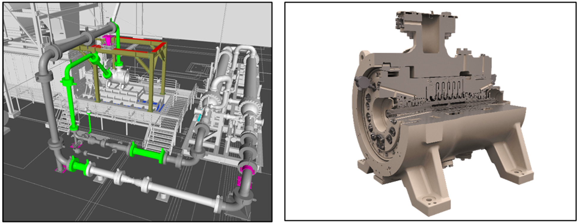
Figure 12.

Full-scale compressor closed loop test schematic and cross-section cut-away of the multi-stage compressor.

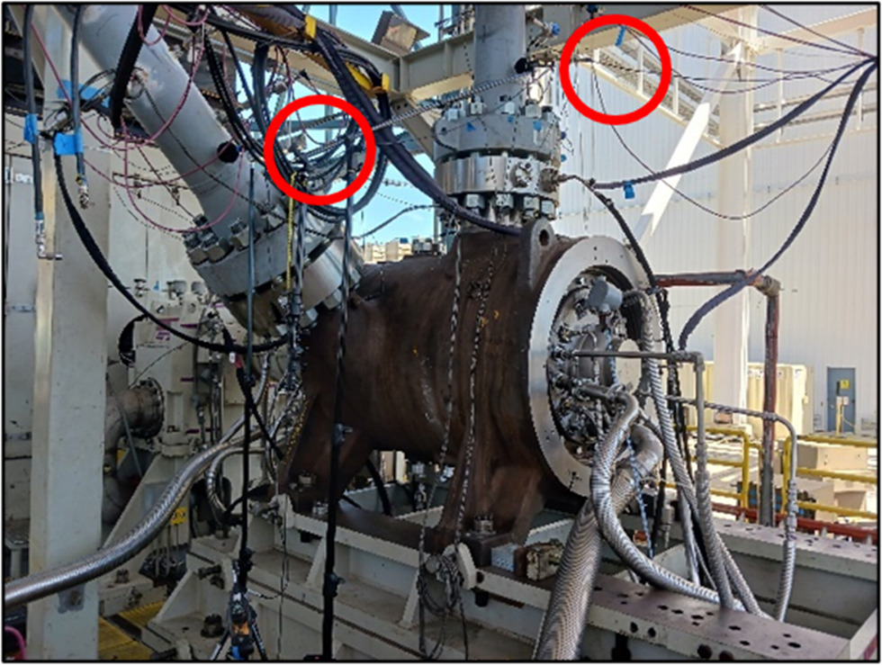
A cross-section view of the subject compressor is shown in Figure 12. The compressor was equipped with microphones on the suction and discharge flanges. The locations of the acoustic devices (positioned ∼0.1 m away from the pipe surfaces) are shown in Figure 13. The microphones were ensured to be Class I Div II compliant in accordance with area classification for the closed loop test facility. The microphones were connected to a Bruel & Kjaer data acquisition system. In addition, dynamic pressure transducers were also instrumented in the inlet and discharge flanges to record the pressure fluctuations arising from the flow-field.

Figure 13.

Centrifugal compressor with highlighted locations of microphones.

The exit stage of the compressor was equipped with a low solidity airfoil diffuser (LSA), comprising of 12 vanes, and exit guide vanes comprising of 8 vanes. The primary purpose of the LSA was to achieve comparable aerodynamic performance at high pressures over a vaneless diffuser, with minimal disruption to the flow range. In addition, the LSA also served as a structural support element to maintain the as-designed diffuser width during operation at high discharge pressures. Aerodynamic performance testing was conducted on nitrogen as the test medium. The as-tested performance on nitrogen at a machine Mach number of 0.42 is shown in Figure 14. The suction pressure was held constant at 500 psia [34.5 bar], and the flow was throttled from the maximum flow condition (near choke) towards minimum flow (near surge). Each flow point was stabilized for a minimum of 15 min to allow for thermal equilibrium to be attained on the compressor. The performance comparison of the as-tested data with and without LSAs is shown in Figure 14. The presence of LSAs results in a minimal reduction to the operating flow range for the compressor, and this is consistent with the results presented in the prior section from the scaled test rig.

Figure 14.

Performance comparison (left), and spectrum color plot of the acoustic measurements.

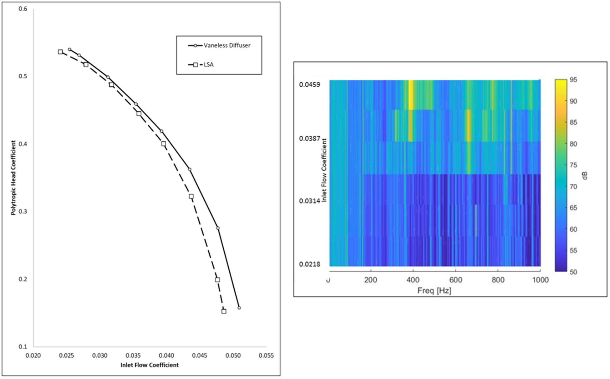
A secondary aspect of the closed loop testing was to benchmark and quantify the aerodynamic (i.e., flow-induced) influence on the compressor vibrations arising from the LSAs. Figure 14 shows the heat map of the acoustic data recorded from the microphone positioned at the discharge flange, as a function of the compressor inlet flow. The acoustic heat map shows a 350–400 Hz component of SPL at 95 dB at maximum flow condition [flow coefficient of 0.0459]. As the flow is throttled towards surge, the magnitude of the sound pressure level drops to below 70 dB followed by a subsequent decay in the magnitude of the 350–400 Hz component.

Figure 15 shows the frequency spectrum obtained from the shaft non-contacting vibration probes (15a) and the dynamic pressure transducers (15b). The concurrent occurrence of the non-synchronous vibration components on the shaft proximity probes, dynamic pressure transducers and the microphones are an indication of a flow-induced forcing function as a source of the excitation. It can be observed super-synchronous frequency component in the 350–400 Hz range appeared on the rotor vibration probes near the maximum flow condition, in addition to showing up on the acoustic microphones. The use of the acoustic microphones and dynamic transducers become evident in this case study, where the shaft vibration probe by itself may not be able to provide additional insight into the source of the vibration. The occurrence of the frequency component on the microphone and pressure spectrums can be used to confirm the flow-induced nature of the vibrations.

Figure 15.

(a) left – frequency spectrum from shaft proximity probes. Left – maximum flow condition (flow coefficient 0.050), right – flow coefficient 0.030; x-axis – frequency [Hz], y-axis – amplitude [mils] and (b) left – frequency spectrum from dynamic pressure transducers. Left – maximum flow condition (flow coefficient 0.050), right – flow coefficient 0.030; x-axis – frequency [Hz], y-axis – amplitude [psi].

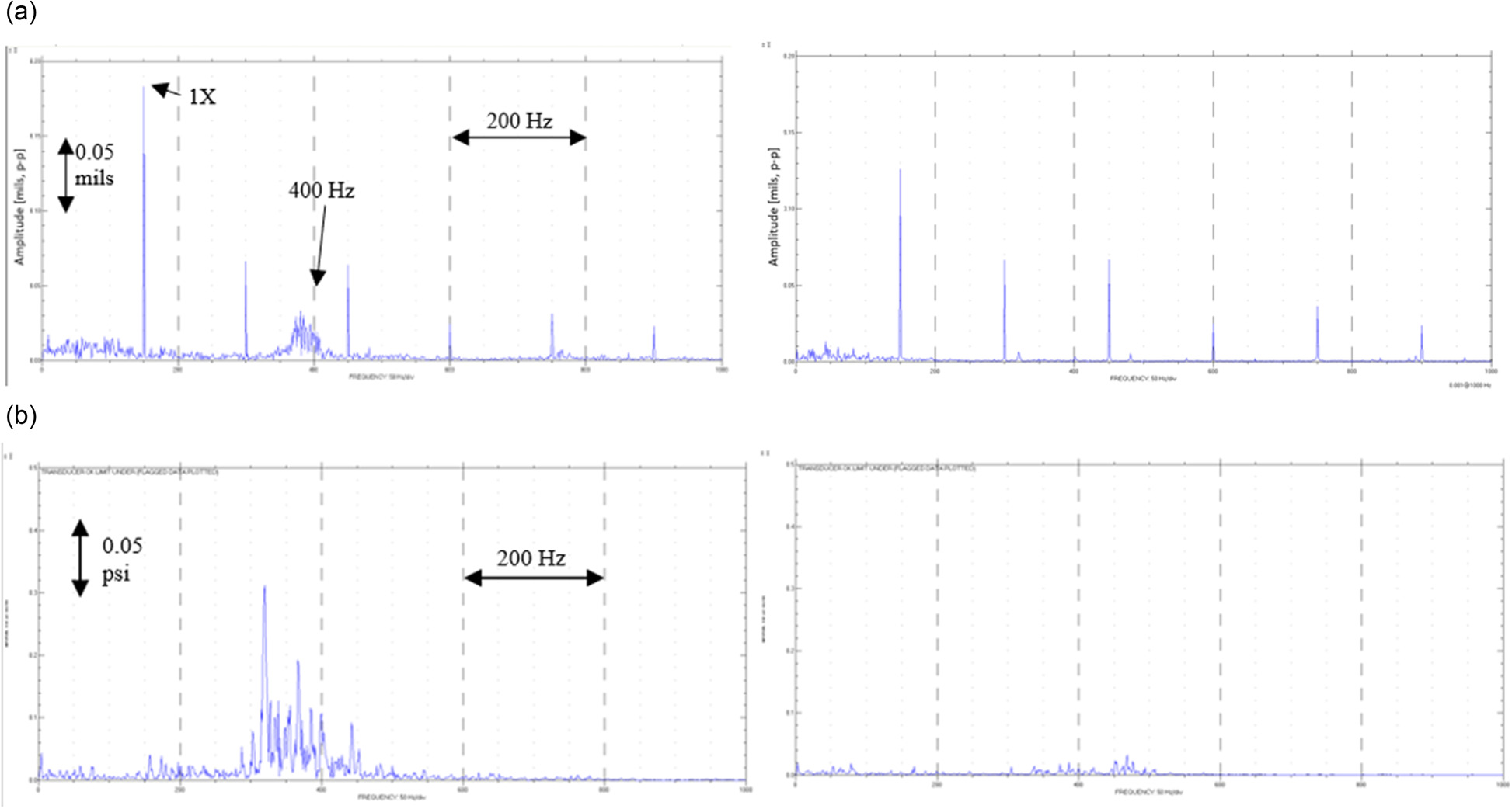
The influence of LSAs on enhancing a blade-pass frequency is well known in the open literature. Most blade-passing frequencies are high enough where it falls outside of the range of shaft proximity probes. Figure 16 is an extension of the heat map shown earlier in Figure 14, with the frequency range extended out to 10 k Hz. The presence of the blade-passing frequency at 2,850 Hz (corresponding to a 19-bladed impeller operating at 9,000 rpm) is evident in Figure 16.

Figure 16.

Acoustic heat map depicting the blade pass frequency.

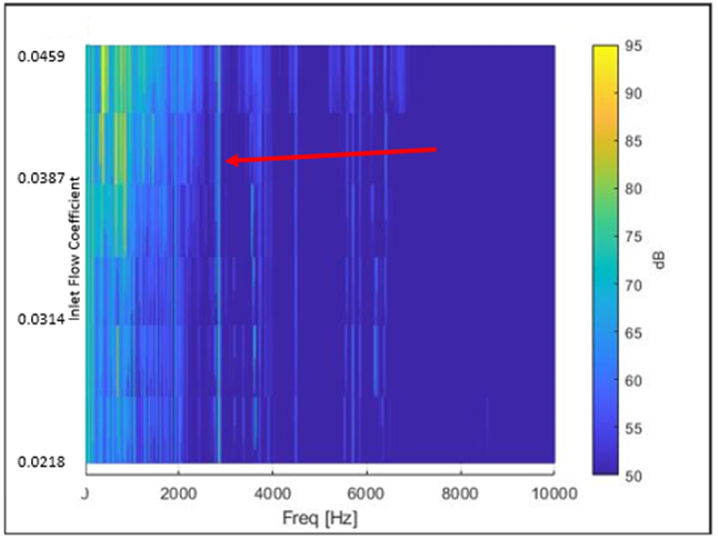
An important observation from Figures 14–16 is that LSAs have the propensity to result in non-synchronous vibrations on the aerodynamic performance map when operating at high flow regimes (i.e., at flows near choke). We can relate this to the wake mechanisms generated downstream of the LSAs as shown in Figure 5. The data presented in Figure 15 shows that the elevated noise levels occur at a flow coefficient of 0.045 or higher. This flow coefficient is beyond 140% of the design flow point at ϕ=0.03. In other words, the occurrence of the elevated non-synchronous and noise levels occur at a flow range that is outside of a typical usable flow range for a centrifugal compressor's field operation.

Conclusions

The aerodynamic performance assessment of centrifugal compressors with low solidity airfoils is presented in this paper. The use of the non-dimensional λ−ϕn2 plot as a design tool for LSAs is outlined. The design aspects of LSAs as related to solidity, stagger angle and radius ratios are presented. Single stage test results from a scaled test rig illustrate the performance comparison in the presence and absence of LSAs. Finally, high pressure full-scale test results from a multi-stage centrifugal compressor are also presented. CFD studies highlight the occurrence of flow separation with LSAs downstream of the vanes. The tested data highlights the occurrence of the non-synchronous vibrations on the high flow side when tested with LSAs.