Rotating test rig

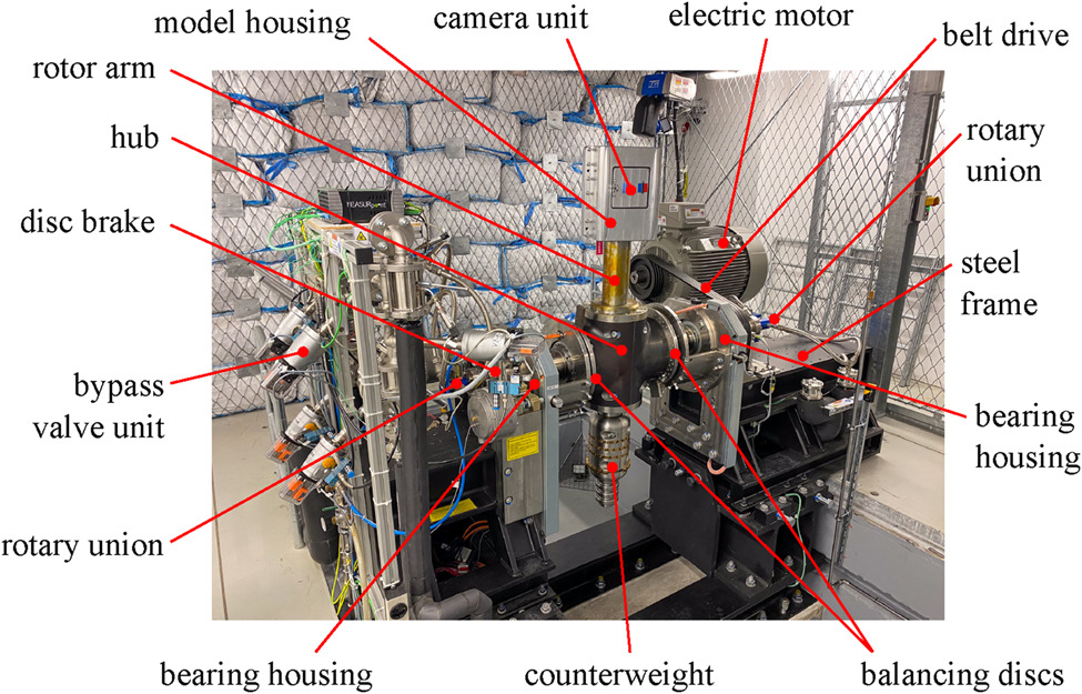
In Figure 1 an overview with the key components of the test rig, which was presented in detail in Waidmann (2020), is shown. In an effort to correctly reproduce the buoyancy effects from the real machine, transient TLC experiments are performed with test air below the ambient temperature. Fluid temperatures as low as −100°C can be achieved for the three air supplies (precool air, tempering air and test air) by means of a heat exchanger operated with liquid nitrogen. Prior to the start of the experiment, precool air (1) is driven through the rotary union at the right hand-side of Figure 1 and flows through the pipes in the hollow shaft and rotor arm. These act as a heat exchanger to the test air pipes, which need to be precooled to a certain temperature so as to minimise heat intake during the experiment, thus facilitating the fluid temperature step change. Tempering air (2) with a temperature equal to the measured test model temperature is directed through the rotary union at the left-hand side of the figure. It continuously flows through the test model in order to pressurise it and to hold constant its initial temperature level. When the rotor pipes reach the desired temperature and the model is pressurised, the electric motor drives the shaft through a belt drive at a speed of up to 900 rpm. Once the target rotating speed, pressure level and test air temperature are reached, the test air (3) is driven through the test model, marking the start of the TLC experiment. This is achieved through a bypass valve unit consisting of six valves which enables the switch between the tempering air and the test air supply. The test air finally exits the shaft through the same rotary union.

Figure 1.

Overview of the rotating rig.

The test bench was designed to enable the accurate setting of the target operating conditions. For this investigation, test cases are classified according to their Reynolds number (Re) and rotation number (Ro). The Reynolds number, determined as Re=m˙dh/Aη, is computed from the cooling air mass flow, the dynamic viscosity determined at the channel inlet location TC0102 (see Figure 3) and the channel geometry. In Ro=ρAΩdh/m˙, Ro represents the ratio of the rotational effects to the inertial forces and is evaluated based on the rotational speed, the channel geometry, the air density calculated from pressure and temperature measurements at the channel inlet (TC0102), and the cooling air mass flow. The test cases in this study are derived from engine-realistic conditions and their operating points are summarised in Table 1.

Test models

Experimental heat transfer evaluation

The experimental method is based on the transient TLC technique, as described in Poser et al. (2007, 2005) and Ireland and Jones (2000). By means of this approach, TLCs are used as temperature sensors and their response times, i.e., indication times, are determined after a sudden fluid temperature change is applied. Through analysis of the pixel-wise TLC indication times and the fluid temperatures, local heat transfer coefficients can be calculated. In the present investigation the TLC type G0C1W with a bandwidth of 1 K from Hallcrest has been applied and calibrated with the stationary calibration method proposed in Poser and von Wolfersdorf (2010), resulting in the indication temperatures presented in Table 1 for the baseline and enhanced geometries.

Heat transfer analysis is performed by means of the in-house code ProTeIn. The first steps involve wavelet-based filtering and adaptive normalisation, as presented in Poser et al. (2009). Following, the time at which the intensity of the green colour channel reaches its maximum, i.e., the TLC indication time, is determined for each pixel separately. The fluid temperature history for each channel position is determined by means of the CFD-based method presented in Gutiérrez de Arcos et al. (2022). The heat transfer coefficient h is calculated through solution of the one-dimensional Fourier heat conduction equation for a semi-infinite solid body and convective boundary condition. However, in order to approximate the actual fluid temperature history, this needs to be discretised through tiny temperature steps ΔTf(j,j−1), and the Duhamel superposition principle needs to be applied. That results in Equation 1:

The wall temperature corresponds to the temperature at the time of indication tind,i.e.Tw=Tind, and the initial temperature is given with T₀. τ_j is given by is a discrete point in time of the fluid temperature history, and ρw,cwandkw are the physical properties of acrylic glass. Heat transfer results are presented in their dimensionless form by means of the Nusselt number Nu=h⋅dh/k(Tf¯) with the local thermal conductivity k(Tf¯) evaluated for the time-averaged local fluid temperature history until the time of indication, and the hydraulic diameter of the first passage dh.

Figure 2.

Schematic view of the fluid domain (left) and test model (right) of the enhanced geometry.

Boundary conditions

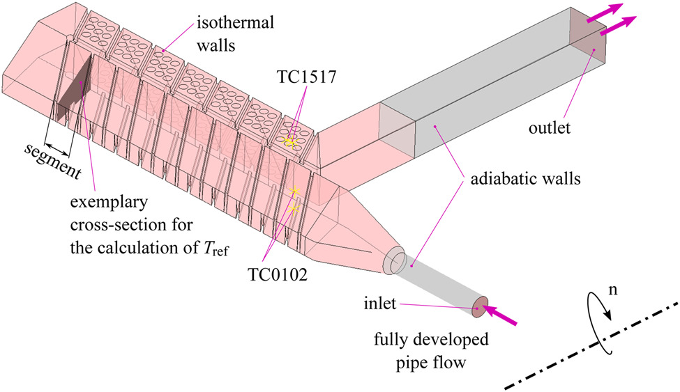
In Figure 3 an overview of the numerical domain with the applied boundary conditions is presented for the enhanced geometry exemplary. Fully developed flow conditions are present at the inlet. The three components of the velocity vector in Cartesian coordinates (X, Y, Z) are derived from a preceding calculation. Furthermore, the inlet temperature stems from the transient TLC experiment as an estimation of the average temperature for the duration of the experiment at the channel inlet, i.e., at the measurement location of the thermocouple pair TC0102. The outlet is characterised with a static pressure boundary condition equal to pout=6bar for all numerical simulations. Considering the channel walls, the no-slip condition is set and a constant temperature equal to the starting temperature of the TLC experiment is applied. Inflow and outflow regions of the channel are modelled as adiabatic walls. Furthermore, the outlet region is extended in order to avoid interference of possible recirculation regions at the boundary location. For cases with rotation, the fluid domain is set a constant rotating speed analogous to the TLC experiment.

Figure 3.

Boundary conditions and experimental TC locations at inlet and outlet of the cooling channel, i.e. TC0102 and TC1517, respectively.

Mesh generation and mesh independence study

The numerical grids were generated in ANSYS ICEM 17.1 (baseline geometry) and ANSYS ICEM 2021 R2 (enhanced geometry) following a multi-block structured approach. The different channel regions were modelled separately in order to allow for a better control of the desired target quality parameters, such as aspect ratio, grid angle and volume change, in accordance with the ANSYS ICEM CFD User’s manual (2021), and dimensionless distance of the first cell adjacent to the wall. In regard to heat transfer, high quality meshes with well-resolved near-wall regions are required. The dimensionless wall distance must not exceed y1+≈1 in order to fully resolve the wall-adjacent region. Furthermore, the cell growth rate perpendicular to the wall is carefully chosen so as to ensure a smooth transition from the walls to the core flow.

On the basis of the aforementioned constraints, a mesh independence study was conducted for the enhanced geometry, following the method proposed in Celik et al. (2008). Through this approach, the Grid Convergence Index (GCI), initially introduced by Roache (1994), is calculated and delivers an estimation for the grid discretisation error of a desired target variable. Three different grids (fine, medium, coarse) with a refinement factor of at least 1.3 are needed, while the first wall cell height is held constant. The study was performed for the area-averaged Nusselt number at the PS, SS and LE channel walls. Depending on the considered channel segment, area-averaged uncertainties can be as high as GCImax=9.7% at PS, GCImax=11.1% at SS, and GCImax=13.1% at LE for the fine grid. For the most part of the cooling channel, however, area-averaged uncertainties are below GCI=5%. The final meshes consist of 11.7 (baseline) and 19.0 million grid nodes (enhanced).

Numerical heat transfer evaluation

Convective cooling is quantified by means of the heat transfer coefficient calculated with Newton's law (Incropera et al., 2017) with

and is made dimensionless with the Nusselt number. In Equation 2 the wall temperature Tw is set as boundary condition in the numerical model and the specific wall heat flux q˙w is a direct result from the numerical simulation. In regard to the Nusselt number Nu=hdh/k(Tref), the hydraulic diameter of the first passage dh is used and is identical for both considered geometries, and the thermal conductivity k(Tref) is calculated at each PS, SS and LE segment for the corresponding reference temperature. The reference temperatures Tref for each PS, SS and LE segment are determined at the corresponding cross-sectional location, defined as the midpoint between the inlet and outlet of each channel segment (see an exemplary segment with its corresponding cross-section in Figure 3). With knowledge of the numerically-obtained bulk temperatures along the cooling channel a dimensionless temperature profile is derived, which is then used to correct the measured fluid temperatures of the TLC experiment through the procedure presented in Gutiérrez de Arcos et al. (2022).

CFD validation

Experimental (EXP) and numerical (CFD) local heat transfer rates are depicted in Figure 4 and have been obtained for the baseline geometry with and without rotation, i.e., at Ro≈0.15 and Ro=0, respectively. They show the heat transfer enhancement relative to the non-ribbed cooling channel from the Dittus-Boelter/McAdams correlation for PS, LE and SS. The flow direction is highlighted at inlet and outlet of the channel with black arrows. In case of the TLC experiment, data for LE is not available. Ribs and the inner wall separator between the first and the second passages (corresponding to a radially outward and a radially inward flow, respectively) have been blanked out.

Figure 4.

Experimental and numerical heat transfer structure (a–d) and segment-averaged heat transfer (e and f) for the baseline geometry under rotation (Ro≈0.15) and without rotation.

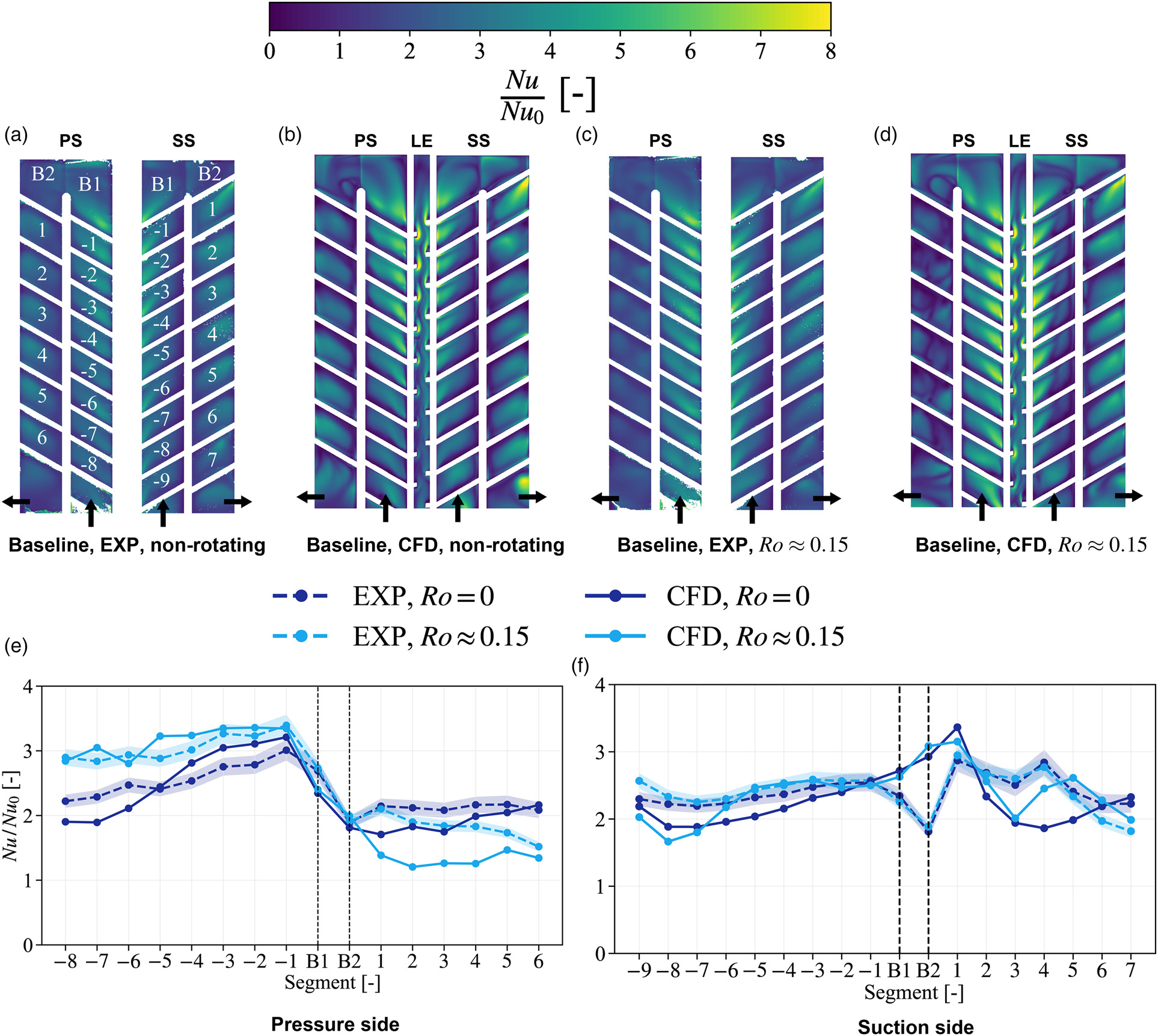
The non-rotating case, displayed in Figure 4a and b, features a heat transfer level that appears to increase towards the bend for the three considered channel regions. From inlet towards bend, a flow pattern consisting of detachment and reattachment to the wall caused by the angled ribs is repeated, as it can be appreciated from both, experimental and numerical results. Moreover, the trapezoidal shape of the first passage translates into generally higher heat transfer for PS than for SS. Directly downstream of the bend, a streak with high heat transfer rates is visible at the first segment of SS as a result of the 180°-turn, which triggers the cooling air impingement onto the SS wall. This structure is visible for both experiment and CFD simulation, however, in the experimental results the streak appears to be weaker in terms of heat transfer level. With disregard to the later point, the second passage is characterised by a monotonous heat transfer structure for PS and SS, and experimental and CFD results align qualitatively well.

As the cooling channel is set under rotation additional sources of momentum arise, altering the secondary flow field and ultimately impacting on the local heat transfer structure. In Figure 4c and d contour plots of the local heat transfer under rotating conditions (Ro≈0.15) are presented for experiment and CFD, respectively. Considering the local structures of the first passage, little change can be observed in comparison with the non-rotating case. Similar to the non-rotating case, heat transfer rates increase towards the bend for the three considered channel regions. There only appear to be changes in the heat transfer level, with a clear enhancement in the rotating case. In contrast to the first passage, the PS second passage features a distinctive pattern which is correctly reproduced by the numerical model, and displays generally lower heat transfer rates than in the non-rotating case. Overall, the qualitative agreement between experimental and numerical results is satisfactory. In order to quantify the deviations between TLC experiments and numerical simulations, data from the contour plots in Figure 4 has been segment-averaged and is displayed at the bottom of Figure 4 by means of XY-plots for PS (left) and SS (right). The flow direction is from left (−8 or −9 at the inlet, respectively) to right (6 or 7 at the outlet, respectively) and the corresponding naming for the different segments is given in Figure 4a. Whereas experimental data is plotted with dashed lines and the respective band with the uncertainty estimation, CFD data is plotted by means of solid lines. At first glance, the main trends observed in the experiment are mirrored appropriately by the CFD data. Considering both experimental and numerical results for the first passage of PS, a deviation below ±12% is reached for the majority of the segments, with the highest discrepancies of −18% for segment −7 in the non-rotating case. Considering the second passage of PS, heat transfer for the rotating case is drastically underpredicted by the CFD, yet a relatively good agreement is reached for the non-rotating case. With respect to the SS, the maximum deviation from the experimental results occurs at B2 and reaches +62% for the non-rotating and +64% for the rotating case, generally with a discrepancy bandwidth smaller than ±20%.

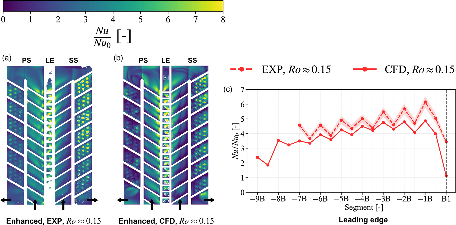
Regarding the enhanced geometry, experimental data for LE is available and can be therefore compared directly with the CFD results in Figure 5 for the rotating case Ro≈0.15, exemplary. In this case, the triangular ribs induce a pattern of diagonal streaks of increased heat transfer for all visible segments. Apparently, their particular shape result in the flow being deflected with a certain angle towards the LE wall, thereby creating a distinguishable heat transfer structure and improving the cooling effect. Analogous to PS and SS for the baseline geometry, heat transfer rates at LE increase from inlet towards bend. They do it in a particular zigzag manner, i.e., higher heat transfer rates for B-segments (e.g. −1B, −2B, −3B, etc.) than for A-segments, as indicated by the segment-averaged data in Figure 5c. A possible explanation for this phenomenon might be given by the trapezoidal cross-sectional shape of the first passage with angled ribs which, in combination with the rotational effect, deflects the flow field from PS to SS, washing the LE. The highest deviation from experimental data occurs at segment B1. In this case, however, due to optical difficulties, the experimental data covers less than half of the considered segment and must be therefore handled with caution. The same applies to segments −8A, −8B, −9A and −9B, which have been blanked out due to insufficient experimental data to draw conclusions. For most of the segments at the LE, the CFD deviation from experimental results falls within a ±15% band, which can be regarded as satisfactory.

Figure 5.

Experimental and numerical heat transfer structure (a and b) and segment-averaged heat transfer (c) for the enhanced geometry under rotation (Ro≈0.15).

Rotationally-induced heat transfer

The integration of leading edge ribs and protrusions in the second passage is expected to alter the secondary flow field and thereby result in heat transfer enhancement. In Figure 6d and e, local heat transfer is depicted in form of Nu(x,y)/Nu0 contour plots for the enhanced geometry in the non-rotating and rotating case (Ro≈0.15), respectively. For a direct comparison, results from Figure 4 for the baseline geometry are displayed again in Figure 6a and b. LE data for the baseline geometry stems from the CFD simulation results. Considering the non-rotating case, a strong increase relative to the baseline geometry is visible for the second passage of PS and SS, with pronounced peaks at the locations of the protrusions, especially at their windward surface. As a consequence of the channel symmetry, both channel sides appear to be similarly affected by the change in the secondary flow field due to protrusions. Likewise, both sides display lower heat transfer rates in the regions adjacent to the inner wall separator (A1), which increase towards the rear side of the channel with the highest peaks at the locations of the protrusions (A2). Through incorporation of LE ribs as an extension of the turbulators at PS and SS, the heat transfer structure completely changes, as observed by comparing Figure 6a and d.

Figure 6.

Experimental heat transfer structure for the baseline (top) and enhanced geometries (bottom) under rotation (Ro ≈ 0.15) and without rotation. LE data for the baseline case stems from the CFD. (a) Baseline, non-rotating (b) Baseline, Ro ≈ 0.15 (c) Baseline, Ro ≈ 0.15 (d) Enhanced, non-rotating (e) Enhanced, Ro ≈ 0.15 (f) Enhanced, Ro ≈ 0.15.

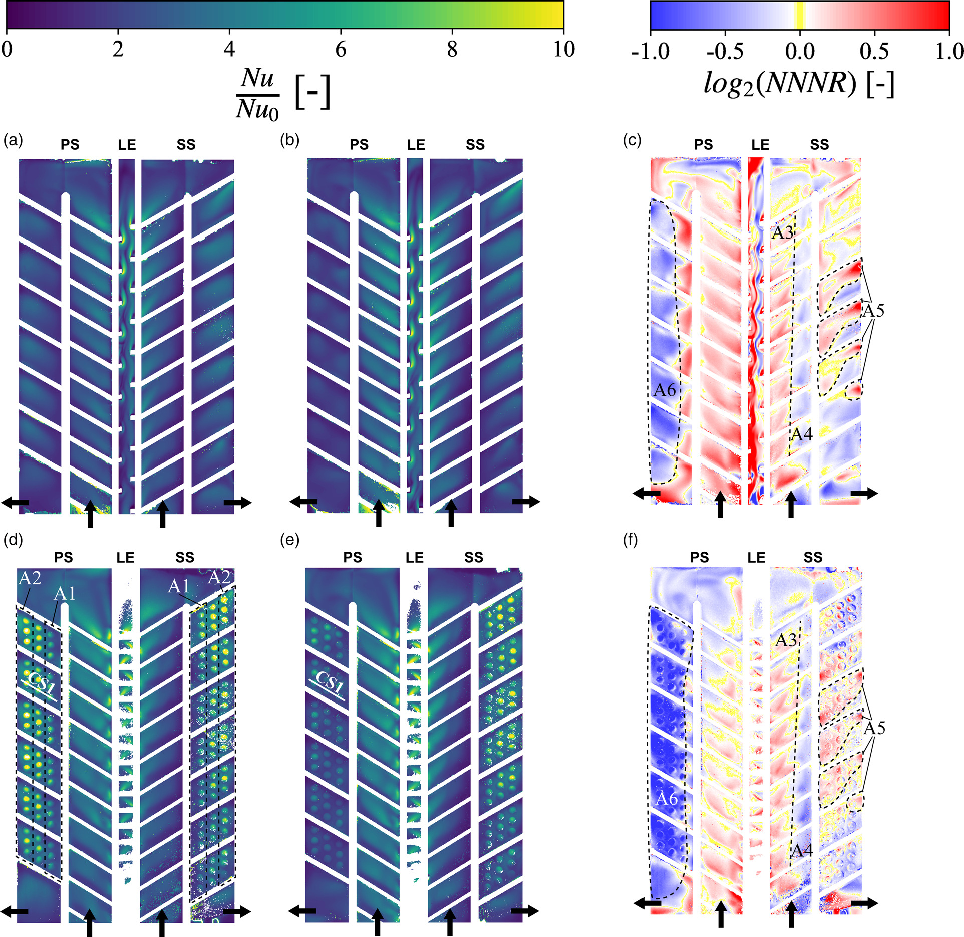
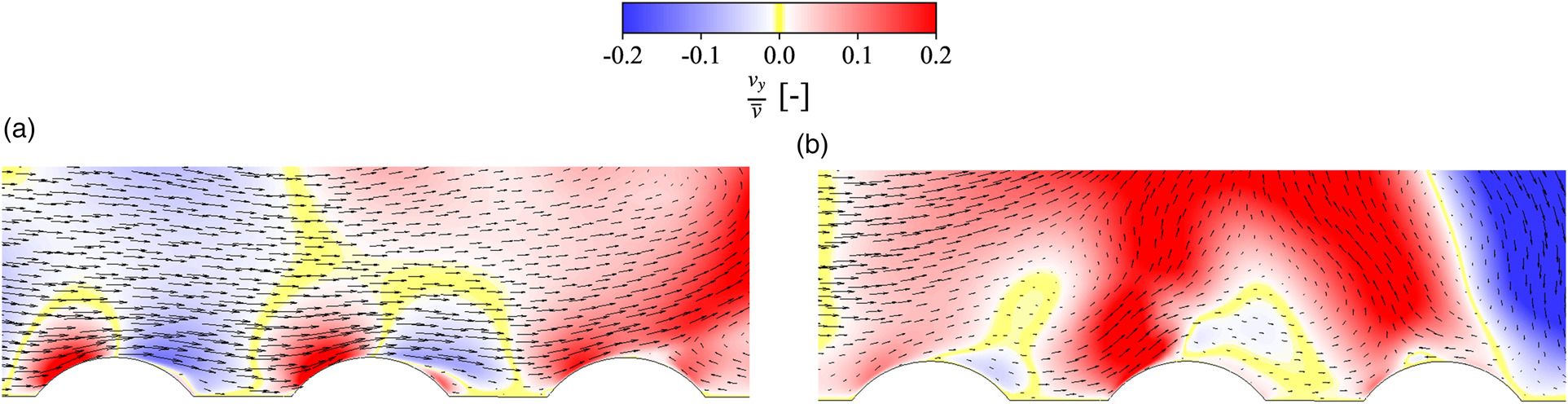
Under the presence of rotation the resemblance between PS and SS in the second passage of the enhanced geometry vanishes. Heat transfer rates remain high for SS, whereas they decrease drastically for PS. This is triggered by the governing Coriolis force direction, which deflects the cooling air from PS towards SS for the radially inward flow. The effect manifests itself in the secondary flow field visualisation from Figure 7, where in-plane velocity vectors in the PS near-wall region over the protrusions are depicted. The corresponding cross-sectional location (CS1) is indicated with a white line in Figure 6d and 6e. Additionally, the wall-perpendicular velocity component v_y has been normalised with the average velocity of the plane (same value for rotating and non-rotating cases) and is displayed as contour plot. The sign, e.g. positive for air flowing towards the protrusions at SS, and magnitude of the vertical velocity component are revealed through application of a divergent colour legend. In the rotating case, the velocity vectors show considerably lower near-wall velocity gradients than in the non-rotating case. Furthermore, in the presence of rotation the Coriolis force lifts the air from the wall, directing to towards the opposite side (SS) and contributing to a reduced heat transfer level at the PS. A similar effect can be assumed for the baseline geometry. The rotational effect can be more clearly visualised through the use of the normalised Nusselt number ratio with a logarithmic scale to the basis of 2. Thereby, the enhancing and diminishing effect of rotation on heat transfer is revealed. In Figure 6c and f contour plots of log₂(NNNR) for the baseline and enhanced geometries, respectively, are depicted. Rotationally-induced heat transfer enhancement is displayed in red; and rotationally-induced heat transfer decrease is displayed in blue. Yellow areas indicate little to no sensitivity to rotation. Whereas variation in the local heat transfer level and structure due to rotation between both geometries for SS is very limited (see A3, A4 and A5), the second passage of PS experiences a remarkable heat transfer decrease (A6), which is in agreement with the lower near-wall velocities noted previously for the rotating case. Furthermore, the rib-protrusion compound of the enhanced geometry intensifies this negative effect, as revealed by the contour plots. Considering the first passage of PS, a lower dependency on rotation exists for the enhanced geometry, as evidenced by the milder rotationally-induced heat transfer pattern. Focusing on the LE of the baseline geometry, a stream of increased heat transfer due to rotation develops from inlet towards bend, with the highest rotationally-caused increase at the channel inlet. The local structure changes completely for the enhanced geometry, where segment-wise zigzag-shaped streaks of increased heat transfer from inlet to bend are observed, with an overall milder rotational effect, compared with the baseline case.

Figure 7.

Detailed view CS1 (see Figure 6d and e) of the secondary flow field structure in the PS near-wall region for the enhanced geometry. (a) Non-rotating (b) Ro ≈ 0.15.

Latin symbols

Greek symbols

Indices

Abbreviations