Experimental setup

The Institute of Turbomachinery and Fluid Dynamics operates a rotating labyrinth seal rig first described in Kluge et al. (2019). This rig permits investigating different turbine shroud cavity geometries experimentally at rotational speeds representative of low-pressure turbines. Kluge et al. (2020), e.g., previously investigated unsteady flow phenomena in the shroud cavity.

The test rig as depicted in Figure 2 employs a rotating disk mounted on a shaft driven by an electric motor. Air enters the rig through a volute inducing pre-swirl with a flow angle derived from the turbine rig described in Henke et al. (2016). The cavity is formed by the seal fin geometry carried by the rotating disk and the outer casing. For the present investigation, two different casing rings were manufactured. Both rings differ only in the area marked Variable geometry in Figure 3 with one ring featuring a smooth rub coating similar to that of a turbine and the other featuring a honeycomb structure.

Figure 2.

Schematic depiction of the rotating labyrinth seal test rig (Rotated by 90°).

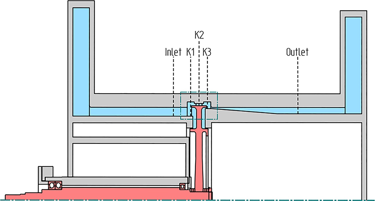
Figure 3.

Measurement positions inside cavity (left) and operating conditions of the test rig (right).

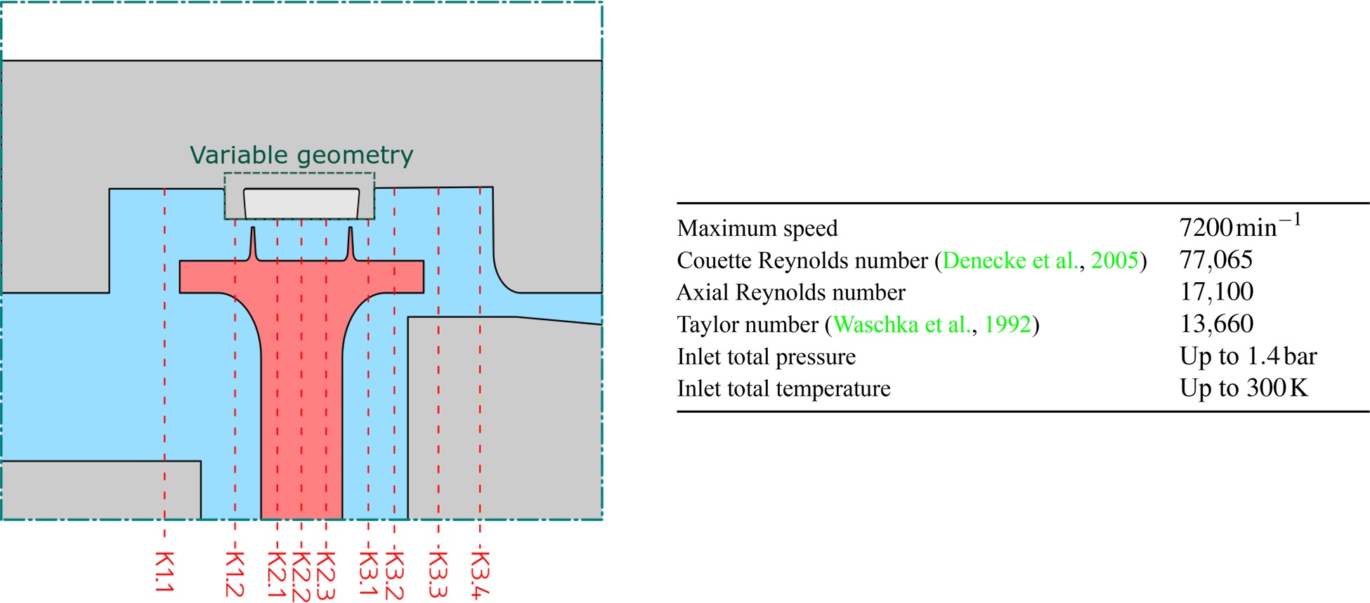
For this investigation of the honeycomb influence on seal flow characteristics, only the cavity geometry deviates from the general rig geometry first documented in Kluge et al. (2019). While the rotor is identical, the casing geometry has been modified. It comprises a constant-annulus section immediately above the rotating disk and two discontinuous changes in diameter upstream and downstream of this section (forward and backward facing steps). The configuration is shown in detail in Figure 3a. The cavity geometry can be subdivided into three sections: The cavity inlet region (K1), the swirl chamber (K2) and the cavity outlet region (K3).

At the rig inlet and outlet planes total pressure and temperature are measured using rake probes while wall taps at the hub and tip casing deliver the static pressure. The mid-span position of each rake is executed as a three-hole probe which yields the respective inlet and outlet flow angles. Additional wall taps line the casing wall at the cavity. Several axial positions—see Figure 3a—are used to obtain the axial pressure distribution, yielding not only the pressure upstream and downstream of the cavity, but also inside the swirl chamber. At K1.1, K2.2 and K3.3 six equidistant circumferential positions exist. For the configuration including the honeycomb structure, additional wall taps were introduced to obtain a more refined pressure distribution. These refinement positions comprise three equidistant circumferential positions. Both K1 and K3 also feature thermocouples near the casing, which are used to measure the change in static temperature across the swirl chamber. Uncertainties within a 95% interval of confidence were obtained for all measurements and derived variables in the experiment.

In order to isolate the honeycomb influence, a constant pressure ratio and corrected rotational speed is maintained for both configurations. Flow and test parameters are listed in Figure 3b. Rotational speeds ranging from nrel=1% to 100% and pressure ratios ranging from Πrel=80% to 100% of those at the nominal operating point were experimentally investigated.

Numerical model

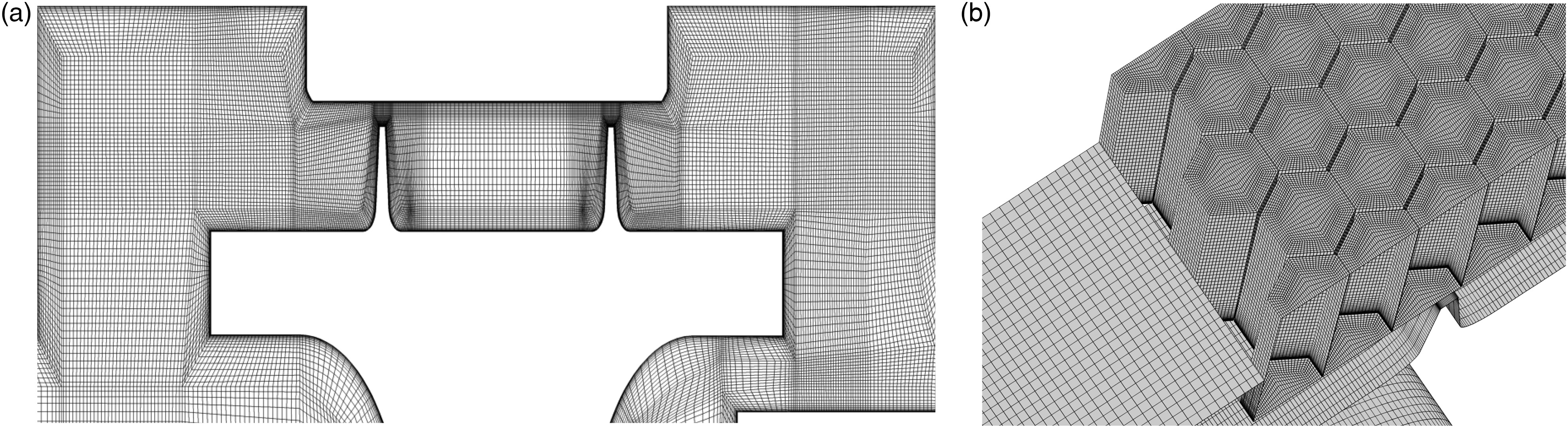
Steady-state simulations have been conducted using the TRACE solver (Franke et al., 2005), which is developed by the German Aerospace Center and MTU Aero Engines AG. The computational grid is shown (distorted for better visibility) in Figure 4. A periodic segment size of 1.5∘ has been chosen for the numerical simulations, as for the steady state simulation no periodic phenomena exceeding a honeycomb pitch (0.75∘) are expected. The segment size thus corresponds to four honeycomb cells in circumferential direction (Figure 4b). The main domain blocking consists of two O-grids wrapping around the hub and casing walls. A dimensionless wall distance of the first grid cell equalling y+<1 is adhered to at every point. A singular honeycomb is meshed using an O-grid and then duplicated to match the manufactured structure. Unlike the main flow domain, the honeycomb walls are not resolved by the grid; instead wall functions are used. The main flow domain comprises 1,770,890 cells while the honeycomb structure totals 4,478,600 cells across all combs.

Figure 4.

Computational grid. (a) Main domain (only every second node shown). (b) Honeycomb grid.

In circumferential direction, a periodic boundary condition is prescribed. The rotor is specified as a moving wall with the absolute speed of the experiment. At the inlet, radial profiles as obtained by experimental data (rake probes) are prescribed while the experimental back-pressure at the casing acts as the outlet boundary condition. The influence of centrifugal forces on the rotor diameter is accounted for by adjusting the radial gap size individually for every investigated speed on the basis of results obtained from structural simulations. For the honeycomb configuration, a fluid-fluid interface connects the main flow domain to the honeycomb domain. This interface allows for the direct transfer of information to the neighbouring domain via interpolation. In case an interface node in the main domain has no partner on the honeycomb side, a local no-slip wall treatment is prescribed instead.

A second-order accurate Fromm scheme (Darwish, 1993) with the van Albada limiter (van Albada et al., 1982) is employed for spatial discretization while a second-order central difference scheme is used to solve the viscous fluxes. The Wilcox 1988 k−ω-model (Wilcox, 1998) is used to model turbulence, using the correction by Kato and Launder (1993) to account for turbulent kinetic energy production near the stagnation points.

The mesh described has been derived by means of a grid independence study in accordance with the guidelines of the ASME V&V Committee (2009). The influence of spatial discretization is assessed by way of the grid convergence index according to Roache (1994), calculated for the discharge coefficient:

The reference grid has been both coarsened and refined by a factor of ℜ32=ℜ12=0.5, i.e. N1<N2<N3. The distance of the first cell to the wall was kept constant when altering the mesh resolution. As per the ASME V&V Committee (2009), a factor of safety FS=1.25 has been used. The relative error ea of the discharge coefficient decreases with grid refinement (Table 1), approximating a logarithmic behaviour. The error relative to the estimated Richardson result (EERE) of the reference grid is EERE32=2.6%. Indeed, the discharge coefficient only changes by 4.9×10−3 when comparing the reference and fine grids. We can thus preclude a significant grid influence on the numerical results obtained on the reference grid.

All simulations featuring a smooth casing converged to an average residual of L1<3×10−7 and a maximum residual of Lmax<1×10−5. Due to the more complex flow interaction, residuals of the honeycomb configuration are higher, equalling L1<5×10−7 and Lmax<5×10−4, respectively.

Effect of honeycomb structures on local flow field

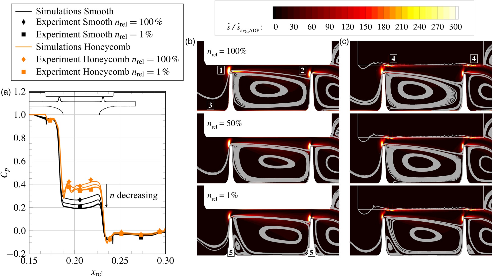
We initially consider the influence of honeycomb structures on the local flow field at the nominal operating point (ADP). The axial pressure distribution through the test rig is depicted in Figure 5 using a pressure coefficient

Figure 5.

Comparison of axial pressure distribution for nrel=100% and Πrel=100%. Error bars indicating 95% confidence interval are smaller than symbol size.

for both experiment and numerical simulation. As mentioned above, the measurement resolution has been refined for the honeycomb configuration while the smooth configuration features fewer measurement positions in axial direction. Comparing experiment and numerical simulation, we are able to demonstrate a high agreement in all measurement planes.

In the flow regions upstream of the first fin and downstream of the second fin the normalised pressure is nearly identical. As is apparent in Figure 5, the key difference is thus the pressure drop across both throttlings, i.e. how the total pressure drop is split across the geometry. For the configuration with a honeycomb structure at the casing, the drop across both sealings is almost equal, while the smooth configuration shows a larger drop over the first seal fin and a smaller drop across the second one. Within the swirl chamber, i.e. between both fins, a deviation in the trend can also be identified. While the honeycomb configuration shows the pressure rising and falling in several sections, the smooth case shows an initially falling pressure followed by a stronger increase immediately upstream of the second fin.

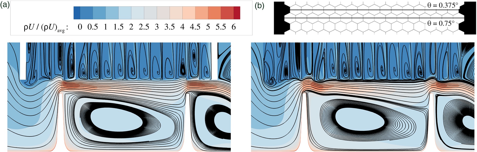
The circumferentially mass-averaged flow field of both the main flow domain and the honeycomb domain inside the swirl chamber is depicted in Figure 6. Upstream of the first fin, the flow field is accelerated due to the forward-facing step, as is evident in the initial pressure drop at xrel=0.18 in Figure 5. A small separation bubble is present at the front section of the inner casing wall. This separation region is smaller for the smooth configuration, as the manufacturing process results in a small chamfer at this location. This chamfer is not present in the honeycomb structure. The flow contraction at the first fin is apparent, resulting in a smaller effective area compared to the actual geometry. At the honeycomb casing, a more complex interaction is visible: Due to the honeycomb structure, the effective flow area is enlarged. In the smooth case, the jet remains attached to the casing wall across the entire swirl chamber. The flow is strongly accelerated across the first throttling, followed by a deceleration upstream of the second fin. The aerodynamic cross-section of the jet increases throughout the swirl chamber. Here, the jet widens considerably more than in the former case. The vortex forming inside the swirl chamber is impacted by the increasing jet area. At the second fin, a similar area increase can be observed for the honeycomb case.

Figure 6.

Comparison of circumferentially averaged flow field in the swirl chamber for nrel=100% and Πrel=100%. (a) Smooth casing. (b) Honeycomb casing.

Based on the geometry of the honeycomb structure investigated, two extreme positions are identified at θ=0.375∘ and θ=0.75∘. Discrete circumferential slices are shown in Figure 7. At θ=0.75∘, both fins are opposite of a honeycomb opening and the effective area at both fins increases. The honeycomb wall immediately downstream of the first throttling, however, radially deflects the jet towards the rotor, “cutting” into the swirl-chamber vortex before again turning towards the casing. This marks a subsequent decrease in effective flow area downstream of the fins. After four combs, the radial flow gradient is considerably diminished and the vortices inside the honeycombs almost act as a smooth boundary. At θ=0.375∘, both fin positions overlap with a honeycomb wall causing a constriction in flow area at the throttling. Since the honeycomb geometry is hexagonal, whenever a honeycomb wall is located above a fin, other circumferential positions feature the widest honeycomb area. The mean area remains constant in circumferential direction. The axial spacing only has a small influence, numerical studies showed no sensitivity to altering the axial honeycomb location. Comparing the detailed flow fields of Figure 7 to the resulting circumferential average in Figure 6, we can infer a net increase in flow area immediately at the fins and a net decrease in flow area downstream of the fins.

Figure 7.

Flow field at discrete circumferential positions of the honeycomb configuration for nrel=100% and Πrel=100%. (a) θ=0.375∘. (b) θ=0.750∘.

Influence of rotation

Additional influences on the local flow field are considered by evaluating the effect of rotation. The nominal operating point (ADP) features the maximum rotational speed investigated. In Figure 8 the axial pressure distributions at differing rotational speeds and at a constant pressure ratio of Πrel=90% are depicted as well as their corresponding circumferentially mass-averaged flow fields. Entropy production is normalized to the mean production at the ADP for the smooth configuration to establish a common reference. The axial pressure distribution in Figure 8a focuses on the section inside the swirl chamber, as no variation exists in the upstream and downstream sections. Rotational speeds considered are nrel=100%, nrel=50%, nrel=10% and nrel=1%. For clarity, only the experimental data of the highest and lowest speeds are included in the plot.

Figure 8.

Influence of rotational speed on pressure distribution and entropy production for Πrel=90%. Error bars in (a) indicating 95% confidence interval are smaller than symbol size. (a) Axial distribution. (b) Smooth casing. (c) Honeycomb casing.

Both experiment and numerical simulation agree well with regard to the axial pressure distribution. The pressure drop again occurs almost equally across both throttlings for the honeycomb case while it is higher at the first fin for the smooth case. The swirl chamber pressure is thus higher for the honeycomb configuration. For both cases, the relative (to the second fin) pressure drop across the first fin increases with a decrease in rotational speed. Additionally, a change in trend inside the swirl chamber can be observed, with the distributions becoming flatter. This effect is more pronounced in the honeycomb configuration, which can be captured by the numerical simulation as well.

Considering the circumferentially averaged flow fields in Figures 8b and c, several characteristic effects can be observed:

Integral parameters

The measured discharge coefficients for various rotational speeds and pressure ratios are depicted in Figure 9. Also included are the numerical results at nrel=100%. As is to be expected, the discharge coefficient decreases for an increase in rotational speed which may be attributed to the contraction of the throttling area at the fins and a reduction of the carry-over of kinetic energy from the first to the second fin due to increased leakage jet dispersion and higher flow losses at the rotating walls. The two lowest rotational speeds (nrel=1% and nrel=10%) almost overlap across the maps. While the numerical simulations are able to predict the pressure distribution across the seal satisfactorily, comparing the discharge coefficient shows significant discrepancies. Kluge et al. (2019) have shown that the discharge coefficient is sensitive to parallel changes in seal clearance, while the pressure distribution is mainly affected by asymmetric differences in the clearance. Thus, a difference in experimental and simulated radial clearance - even one within the measurement uncertainty of the clearance - may account for the offset.

Figure 9.

Discharge coefficient for smooth (left) and honeycomb (right) configurations. Error bars indicate 95% confidence interval.

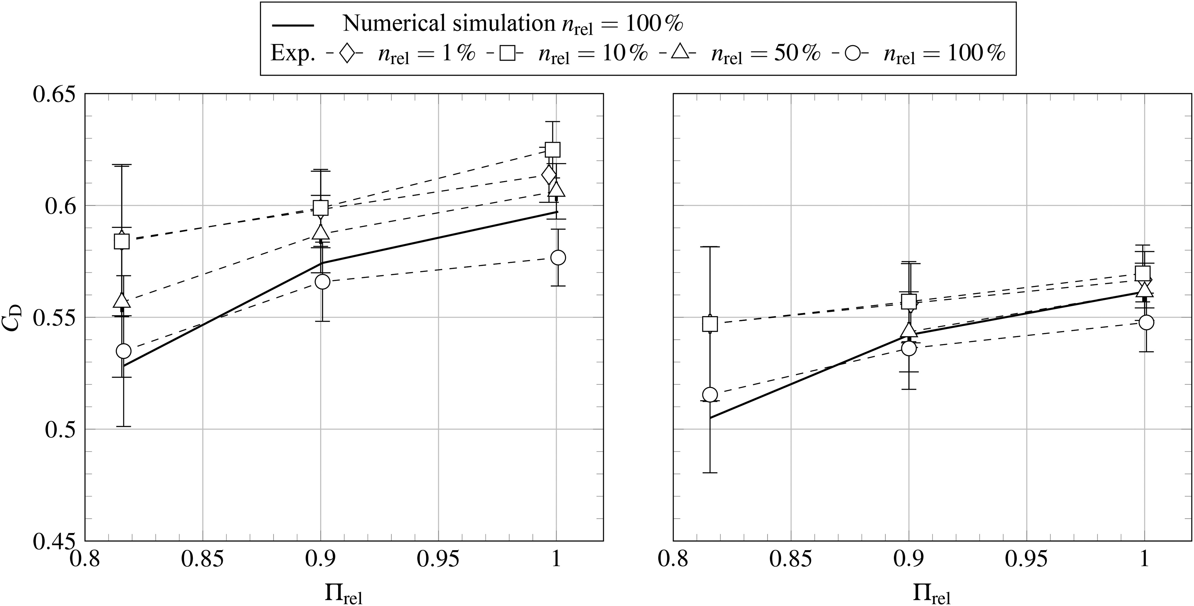
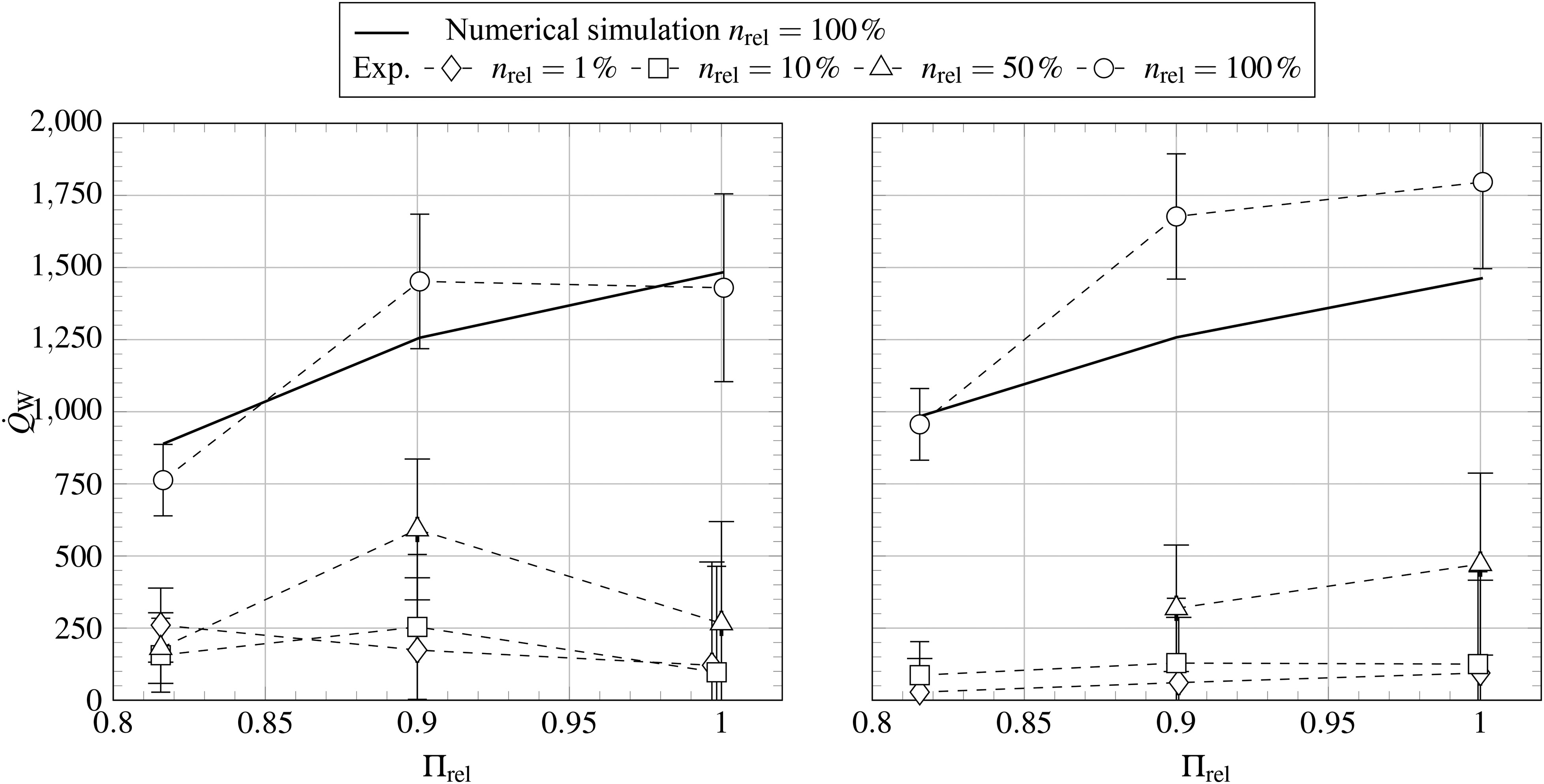
The discharge coefficient of the investigated honeycomb structure is lower than that of the smooth configuration for all speed lines investigated. While the total pressure drop remains the same, the mass flow rate through the labyrinth seal decreases, in line with the observed higher losses. Considering windage heating (Figure 10), higher dissipation of kinetic energy is apparent. At the nominal operating point, the temperature difference between the boundaries of the control domain increases by 37% in the experiment. As the mass flow rate decreases by 8%, windage heating as the product of both contributions increases. A similar trend exists for all operating points along the nominal speed line. For operating points at lower speeds, differences are considerably smaller. Since the jet inside the swirl chamber was shown to increase in size if the rotational speed increases, friction between it and the swirl-chamber vortex are likely the main driver for loss, in addition to the local dissipation at the honeycombs. The sensitivity to honeycomb structures is, however, much lower in the numerical simulation, where the calculated windage heating is almost the same for both configurations.

Figure 10.

Windage heating for smooth (left) and honeycomb (right) configurations. Error bars indicate 95% confidence interval.

Even though the numerical simulations were demonstrated to capture the pressure drop across the labyrinth seal well, the prediction of integral parameters shows considerable deficits. Only for the lowest pressure ratios of the smooth and honeycomb configurations a good agreement can be found. At the higher pressure ratios, the discharge coefficient is over-predicted by 3.6% for the smooth and 2.6% for the honeycomb configuration. Previous investigations (Kluge et al., 2019) have demonstrated a considerable impact of the gap size on the mass flow rate while RANS-models are known to mis-predict the dragging effect of the rotor (Wein et al., 2020) which becomes more pronounced for high rotational speeds.

Finally, we consider the ability of empirical correlations to predict the mass flow rate of the labyrinth seal. Figure 11 depicts the mass flow rate relative to that at the nominal operating point for the smooth-casing configuration, i.e., m˙ref=m˙ADP,smooth. Included is the mass flow rate as predicted by the correlation by Egli (1935) using the parameters introduced in the methodology section of this paper. For the smooth configuration, the predicted mass flow rate agrees well for the entire map, albeit the sensitivity to the change in rotational speed appears lower than in the experiment. The deviation to the experimental data equals 3.4% for maximum speed and pressure ratio. For the honeycomb configuration, mass flow is consistently over-predicted across the entire map as a result of not accounting for the change in the effective gap size and increased losses in the swirl chamber when using the original formulation of Egli's correlation. Using the numerical results presented in this paper, we can derive a simple a-posteriori correction for the correlation. Based on the case of nrel=1%, the effective area changes compared to the smooth configuration can be obtained by evaluating Fig. 8. Since the gap area Agap remains constant, the flow coefficient becomes a function of jet area only. We observe As the jet wides up to a higher degree for the honeycomb configurations, we obtain a factor of ξ=(αHC/αSmooth)=1.35. With the minimum flow area increasing to a lesser degree than the jet area, the contraction coefficient CC=(Am/A1) decreases, ψ=(CC,HC/CC,Smooth)=0.63. Introducing both factors to modify Egli's correlation yields

Figure 11.

Mass flow rate for smooth (left) and honeycomb (right) configurations. Error bars indicate 95% confidence interval.

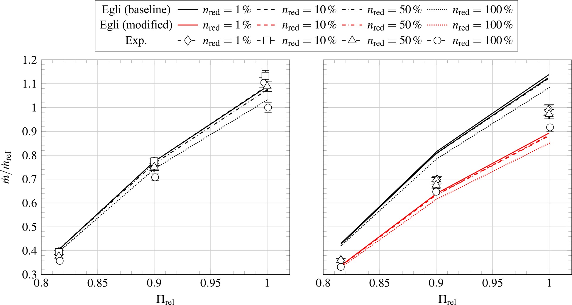
The results of this modification are included in Figure 11. For low rotational speeds, the modified correlation matches experimental results. For higher speeds, deviations increase as the correction factors were only obtained close to zero speed and prescribed for all operating points. This neglects the influence of rotation on dissipation and momentum (widening of the leakage jet) discussed previously. Obtaining correction factors in each operating point could enable a better prediction, but would require pre-existing results and thus defeat the purpose of such a correlation. It can nevertheless be demonstrated, that a correlation is possible when accounting for the effects discussed in this paper.

Latin symbols

Greek symbols

Subscripts

Abbreviations