
Introduction
Diffusers make an essential contribution to increase the efficiency of power-generating steam and gas turbines. They harvest the otherwise wasted kinetic energy of the turbine exhaust flow and convert it into pressure-volume work, i.e., an increase in static pressure. For a given static outlet pressure a diffuser enables a higher turbine pressure ratio, resulting in an increase in power output. As the heat input of the thermodynamic cycle remains constant the thermal efficiency increases as well. The primary aerodynamic design goal of an exhaust diffuser is to maximise the kinetic energy conversion of the turbine outlet flow. The effectiveness of this process can be evaluated using the dimensionless pressure recovery cp defined as
Assuming an ideal flow, it can be shown that an infinite area ratio AR of outlet to inlet area is required to convert all kinetic energy of the flow into static pressure. For such an ideal diffuser, the pressure recovery coefficient is defined as
where
The outlet flow of a real exhaust diffuser with a finite area ratio has residual kinetic energy. This kinetic energy is characterised by the kinetic energy coefficient ξ
In contrast to an ideal inviscid flow, real thermodynamic processes are not completely reversible and thus entropy is created. This creation of entropy is tantamount with a loss of total pressure. A dimensionless total pressure loss coefficient can be defined as
It can be shown per the Bernoulli equation that cp, ξ, and ζ are related via
Equation (6) shows that within the pressure budget a decrease in total pressure loss results in a change of pressure recovery and kinetic energy coefficient. Two respective examples of this interdependence shall be given:
The pressure recovery primarily depends on the diffuser geometry, see Equation (2). Shorter diffuser designs are advantageous as the shorter flow paths result in less frictional total pressure losses. Additionally, shorter diffusers yield reduced investment costs. Given a constant area ratio, as the length of a diffuser decreases, its opening angle becomes steeper and the diffuser flow becomes more prone to boundary layer separation, which is a source for total pressure loss.
The residual kinetic energy is often considered as unexploited energy when focusing solely on pressure recovery, but in context of a power plant, kinetic energy is required to drive the flow through the exhaust stack downstream of the diffuser. This is especially important if the gas turbine is operated in a combined cycle where a heat recovery steam generator follows downstream of the diffuser. This type of component introduces a considerable flow resistance within the flow path, where lots of kinetic energy is dissipated. Therefore a certain amount of residual kinetic energy is essential for the overall process.
In conclusion, there is a strong interdependence between total pressure loss, pressure recovery and residual kinetic energy: an overall reduction of total pressure losses benefits the diffuser design, in particular if the diffuser is considered as a part of a highly integrated system, like power plants. We consider a combined approach towards the design and its adjacent components to be of cardinal importance.
Stabilisation number
A basis for evaluating the pressure recovery of a diffuser design are empirical diffuser charts, e.g., Sovran and Klomp (1967) or ESDU (1990). However, these charts rely on simplified inflow conditions and require additional, semi-empirical corrections to account for non-uniform inflow conditions. For example, Vassiliev et al. (2011) showed that the diffuser performance depends on the inlet Mach number, total pressure distribution, flow angle, and turbulence characteristics.
In addition to the static inlet conditions Kluß et al. (2009) numerically investigated the effects of unsteady wakes and secondary flows shed from rotating cylindrical spokes upstream of the diffuser on the pressure recovery. In contrast to predictions made using diffuser design charts assuming static inlet conditions, the unsteady inflow caused a re-attachment of the boundary layer. This results in an increase in pressure recovery exceeding static predictions. The findings were experimentally validated by Sieker and Seume (2008). Kuschel and Seume (2011) conducted additional experiments using a NACA profile instead of cylindrical spokes. A detailed analysis of these experimental results can be found in Kuschel et al. (2015) and Drechsel et al. (2015). They conclude that the increase in pressure recovery is caused by the interaction of tip vortices of the rotor blades with the diffuser boundary layer. The origin of theses vortices in the rotor tip region is further investigated by Drechsel et al. (2016). All these findings show that a combined design methodology for the last turbine stage and the diffuser is beneficial in achieving more efficient designs.
The stabilising properties of tip leakage vortices generated in the last rotor row and their effect on the boundary layer characteristics have been examined in Mimic et al. (2018). A correlation between the pressure recovery of the diffuser and integral rotor parameters of the last stage has been established, based on analytical considerations, numerical simulations, and experimental data. Parts of the experimental data have previously been published in Kuschel (2014). These rotor parameters are loading coefficient Ψ, flow coefficient Φ, and reduced frequency fred (see Equations A1 to A3, as detailed in Appendix A).
Both experimental data and scale-resolving simulations, carried out with the SST-SAS method, showed excellent agreement with the correlation. The three parameters have been further condensed into the stabilisation number Σ which is defined as
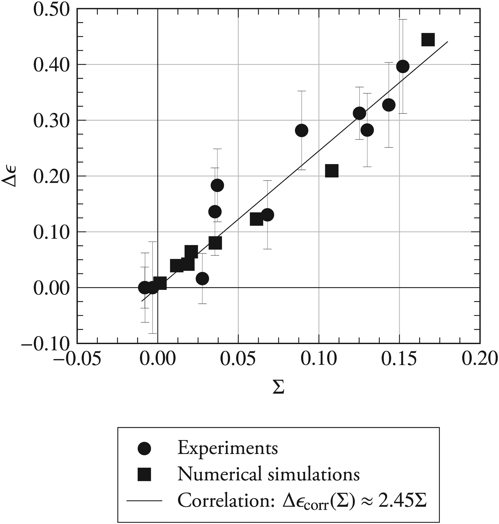
The number represents a measure for the prediction of the diffuser effectiveness
as depicted in Figure 1. The correlation shows that operating points with higher values for the stabilisation number Σ—i.e., essentially higher blade loading, more circumferential trajectories of the blade tip vortices, and more vortex passings per unit time—exhibit an increased diffuser effectivity. A change in Σ can be attributed to deliberate blade design choices regarding the last turbine stage as well as part-load operation for a given engine design.
Figure 1.
Increase in diffuser effectiveness from reference, Δ ϵ
Total pressure loss coefficient
The total pressure loss in diffusers can be attributed to several sources. From a design point of view the losses caused by struts within the flow path, especially with high incidence flow during part-load, and the losses in the Carnot diffuser between the annular and conical diffuser are of great interest. The great amount of research conducted makes this evident, see for example Hirschmann et al. (2012), Vassiliev et al. (2014), Schäfer et al. (2014) or Seume and Drechsel (2015). In this paper, however, we consider just the annular part of the diffuser without struts.
The scope of this paper comprises the total pressure losses produced in the shroud boundary layer of the annular diffuser downstream of the rotor. Babu et al. (2011) were able to demonstrate that rotor tip leakage, achieved by means of flow injection in the shroud region, allow to decrease total pressure loss in comparison to an idealised uniform inflow. In the investigation presented here, the tip jet is achieved by a rotor instead. Therefore, a trade-off can be expected between the losses introduced by the tip vortex and the loss reduction by the homogenisation of the boundary layer and its delayed separation. As flow separation can generally be linked to a decrease in pressure recovery and an increase in total pressure loss, we propose the following hypothesis:
The total pressure loss coefficient ζ decreases for increasing values of the stabilisation number Σ.
Note that because this investigation takes place immediately downstream of the rotor, additional mixing losses, that are introduced by the wakes of the rotor entering the diffuser domain, must be taken into account.
Analytical considerations
According to Denton (1993), losses in turbomachinery can be divided into three categories: profile losses, endwall losses and leakage losses. In this paper, leakage losses do not play any significant role, as the diffuser discussed is a rather simplified model. In order to give a better representation of the flow phenomena in the diffuser, the remaining loss mechanisms can be rearranged into:
The first two loss mechanisms work in conflict: the vortical structures incoming from the rotor blade tips do reduce boundary layer thickness, even preventing separation and, as such, cause a reduction of boundary-layer-related losses. However, at the same time, these vortical structures can be shown to increase the secondary flow losses. In order to present a proper budgeting of the two adverse influences, a closer look shall be taken at the underlying flow mechanisms.The third loss mechanism—the mixing of wakes incoming from the turbine—is somewhat different: because the factors, i.e., width, deficit, and shape of the wakes that determine the mixing losses are strongly dependent on the rotor geometry, the exact interactions are beyond the scope of this paper. We do, however, propose a rather simple rectification of the wake-induced losses for the given configuration later in this composition.
Boundary layer losses
For an ideal gas, the energy equation of a flow can be given in the following form:
where sij is defined as the traceless strain rate tensor, i.e.,
The last term
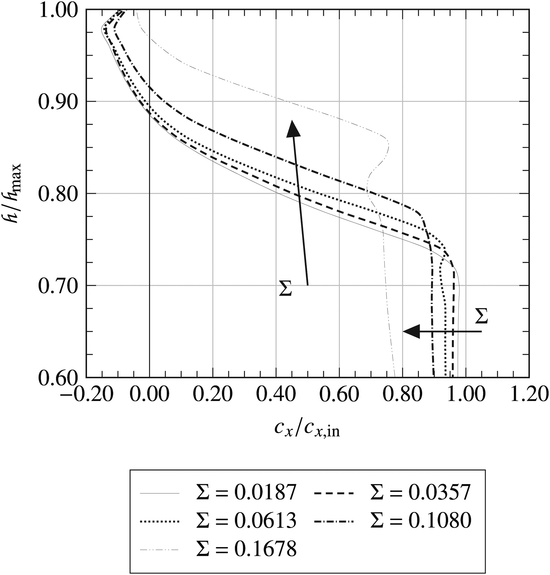
Figure 2.
Mass-flow-weighted, circumferentially averaged radial profile of non-dimensional axial velocity at 50% of diffuser length (Reproduced from Mimic et al., 2018).
Secondary flow losses
While the increased diffuser effectiveness and reduced total pressure losses in the boundary layer are certainly favourable, the effect of additional secondary flow structures in the diffuser would benefit from further examination. From the dot product of the vorticity ωi and the vorticity equation, i.e.,
follows the enstrophy equation, namely
with the enstrophy
and giving a measure for the rotational kinetic energy of the flow field. Here, the last term on the right-hand side of Equation (12),
Note, however, that dissipation of energy and dissipation of enstrophy should not be understood as two summands of some kind of total, or combined, dissipation. The same as enstrophy describes a filtered feature of the velocity field, namely its rotation, the dissipation of enstrophy gives a measure for the portion of energy dissipation that is caused by said rotation.
Because the interactions between the boundary layer in the diffuser and the blade tip vortices are complex and not necessarily linear—meaning that they cannot simply be superimposed onto each other—a mere analytical prediction would be inaccurate, at best. Therefore, we present experimental data and numerical simulations to evaluate the extent of the individual influence factors and to assess their effect on overall total pressure loss production.
Test facility
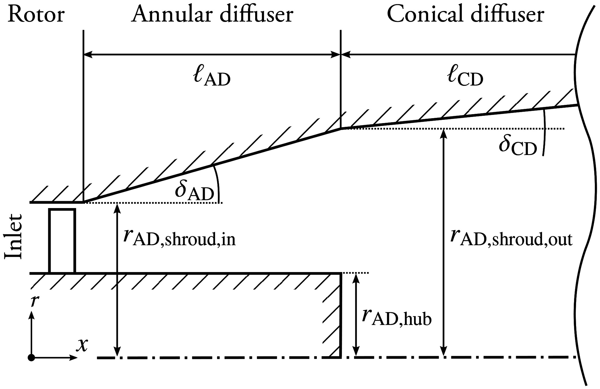
Experimental investigations were carried out on the low-speed axial diffuser test rig at the Institute of Turbomachinery and Fluid Dynamics. The test rig represents a heavy-duty exhaust diffuser at a scale of 1:10. The diffuser is divided into an annular and a conical section, as shown in Figure 3. The half-opening angle δAD of the annular section is 15°. The boundary layer of the annular diffuser is susceptible to separation for steady homogeneous inflow conditions, according to the diffuser charts of Sovran and Klomp (1967). A rotating wake generator provides inflow conditions for the diffuser, similar to the conditions at the outlet of a low-pressure turbine. Two interchangeable rotating wake generators are used, that consist of 30 and 15 symmetric NACA0020 blades, respectively. The aerodynamic blade loading equals zero at design operating conditions. Additional test rig parameters can be found in Table 1.
Numerical method
All presented simulations were carried out using the non-commercial solver TRACE 8.2 (Turbomachinery Research Aerodynamics Computational Environment). TRACE is developed by the Institute of Propulsion Technology at the German Aerospace Center (DLR). Turbulence is modelled using SST-SAS and fully turbulent boundary layer treatment at the walls. SST-SAS describes the combination of the Scale Adaptive Simulation (SAS) method by Menter and Egorov (2010), and the k–ω-SST turbulence model by Menter (1994) and is used to facilitate the formation of unsteady flow structures such as boundary layer separations and vortices. A stagnation point anomaly fix according to Kato and Launder (1993) is employed. A blending function from Strelets (2001) is used, in order to switch between a second order central differencing scheme in SAS-dominated flow regions and a second order upwind differencing scheme in RANS-dominated flow regions. The object is to reduce numerical dissipation in the former and to enhance stability in the latter. Further details concerning the numerical setup are explained in Mimic et al. (2018).
Computational domain
The numerical domain represents one pitch of the rotor. The numerical simulations feature—different than in the experiments—blade counts of 25, 30 and 40. The blade has a symmetric NACA0020 profile and is unloaded at the aerodynamic design point. The rotor domain is followed by an annular diffuser with a half-opening angle of 15° leading to a numerical outlet section that is made up of a divergent and a straight duct. The entire numerical domain, as shown in Figure 4, is in a rotating frame of reference. The numerical reference planes for the evaluation of the overall diffuser total pressure loss coefficient ζ match the experiment. They are located 15 mm downstream of the diffuser inlet and at diffuser outlet.
Figure 4.
Computational Domain (coarse mesh for display): The entire domain is simulated inside the rotating system (Reproduced from Mimic et al., 2018).
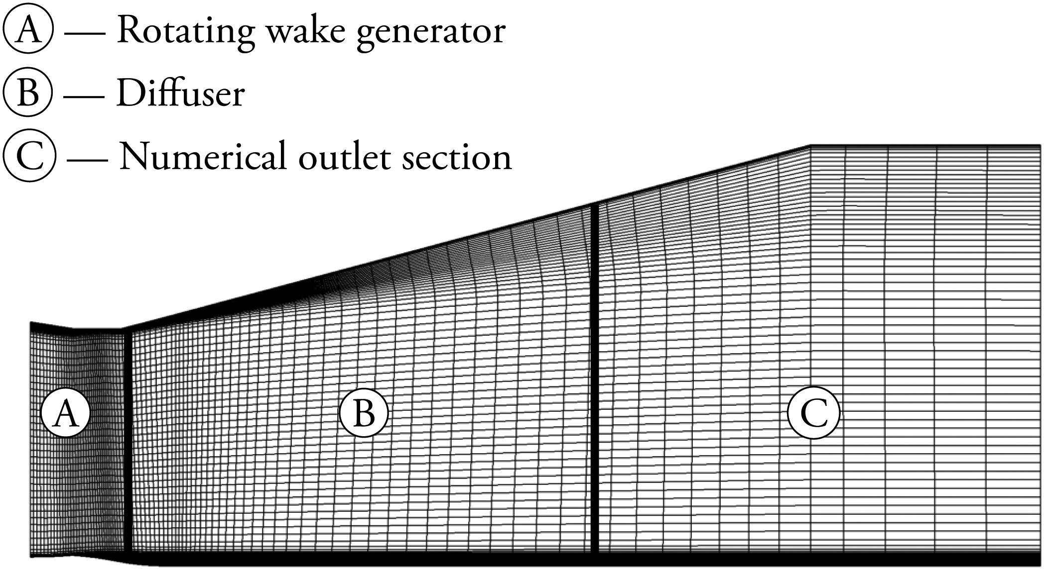
The mesh consists of 1.7–2.4 million overall cells, depending on the blade count of the respective mesh. The mesh is refined in and around the tip gap as well as in the diffuser shroud region. Here, unsteady effects are to be expected due to vortex generation and massive boundary layer separation. A numerical outlet section—downstream of the nominal diffuser outlet—coarsened in axial direction leads to locally elevated numerical dissipation. This way, eventual disturbances interacting with the outlet boundary condition are damped. Numerical convergence and stability are enhanced, as a result. Because the whole numerical domain is part of the rotating relative system, no interface is needed between rotor and diffuser. Static pressure values are given as outlet boundary conditions. The outlet pressure is adjusted to match the required mass flow rate for each individual operating point. An extensive grid convergence study with a similar grid and the SST model has been carried out by Drechsel et al. (2015).
Analysis
We present a range of operating points differing from each other in Ψ, Φ, and fred by varying the blade count n, rotor speed N, and mass flow rate
Table 2.
Test cases (Mimic et al., 2018).
Samples № 3, 6, and 11 are essentially incidence-free and exhibit no turning. The negative values listed for № 3 and 6 are most probably due to measurement inaccuracies, which are negligible. Hence, variants № 3 and 6 are used as the respective references for the experiments; sample 11 represents the reference for numerical simulations. For all cases examined, the flow coefficient is equal to or greater than the design flow coefficient at reference conditions, resulting in a change in incidence. The work coefficient is mostly greater than zero, as this would be expected for a turbine.
Rectified total pressure loss
The absolute rotor outflow angle α depends on the operating point. Thus, the fluid travels a longer distance in the diffuser with regards to a swirl-free rotor outflow. Trigonometry shows that the length of a streamline is inversely proportional to cos α. Because total pressure losses are expected to increase with the distance covered, the total pressure loss coefficients for the respective operating points are rectified to an equivalent, swirl-free pressure loss coefficient.
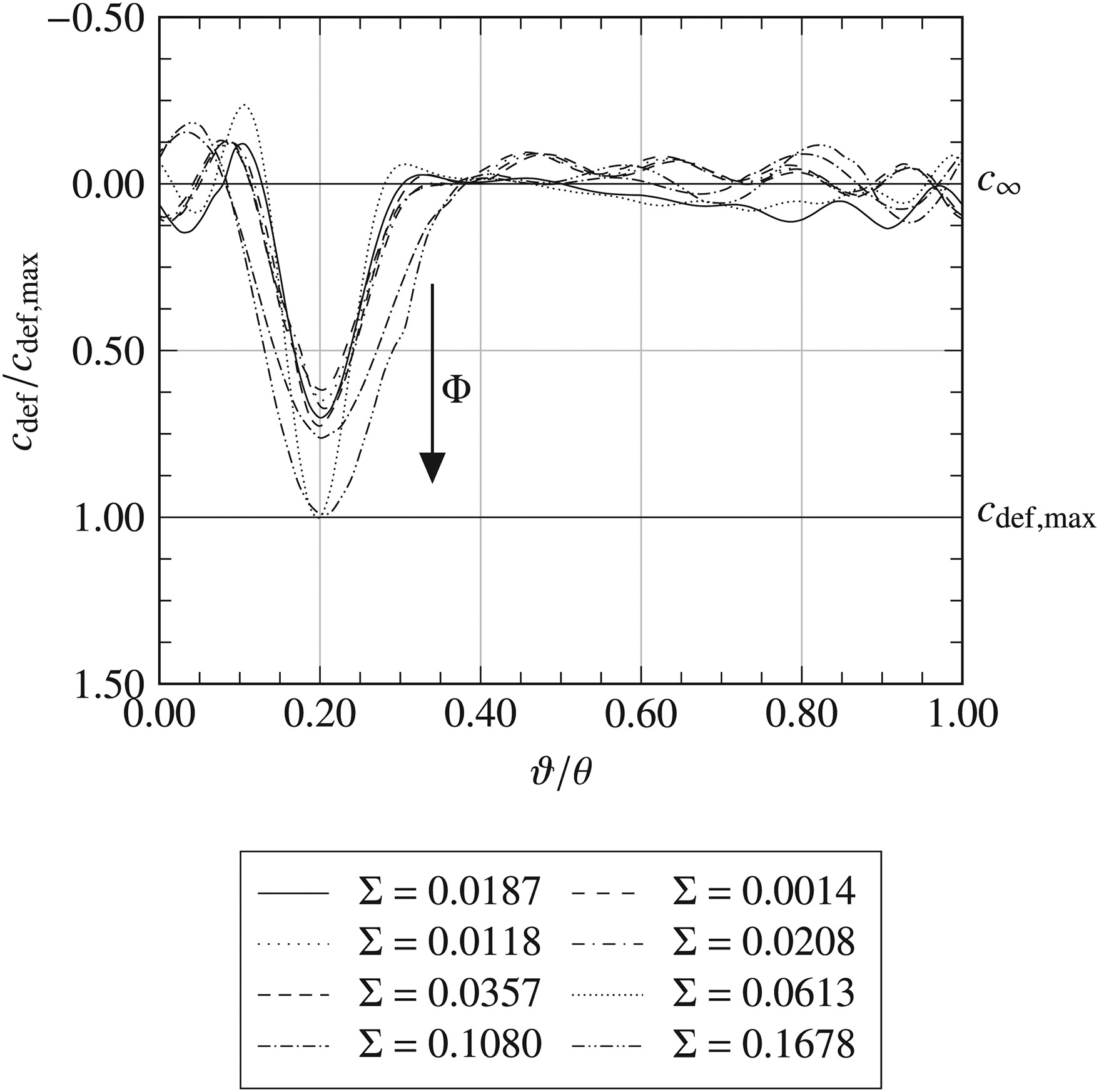
Because the definition of the stabilisation number Σ is based on the behaviour of the tip leakage vortices, it cannot account for the effect of wakes generated by the rotor. A simple numerical analysis reveals that the wakes become more accentuated for higher flow coefficients Φ—this equals a higher incidence of the rotor inflow—which manifests in greater wake velocity deficits as shown in Figure 5. As can be seen, some oscillations are present in the free-stream region. Even though they bear no significance on the overall result, this is a typical issue that arises when RANS computations are performed using central differencing schemes. It is caused by inaccuracies in the performance of the blending function from Strelets (2001).
Figure 5.
Time-averaged circumferential distribution of non-dimensional wake velocity deficit at Euler radius at 8% of diffuser length.
Additionally it is assumed that the pressure loss coefficients associated with wake mixing are roughly proportional to the square of the absolute rotor outflow velocity
where
Note that the relative rotor outflow velocity
Of course, the assessment of wake mixing losses can be done in greater detail, which is, however, beyond the scope of this paper. Examples for such calculations are given by Denton (1993) as well as Rose and Harvey (1999).
The correlation
Figure 6 shows for the numerical simulations performed that the rectified diffuser pressure loss coefficient
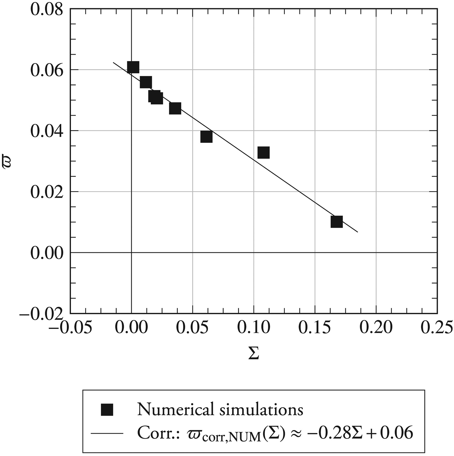
It is, however, physically impossible for
The absolute difference in rectified total pressure loss coefficient to the respective reference variants for simulations and experiments,
facilitates the comparison between record sets. The result is shown in Figure 7. Again, a linear correlation for both, experiment and numerical simulations, between
Figure 7.
Absolute difference in rectified diffuser total pressure loss from reference, Δ ϖ
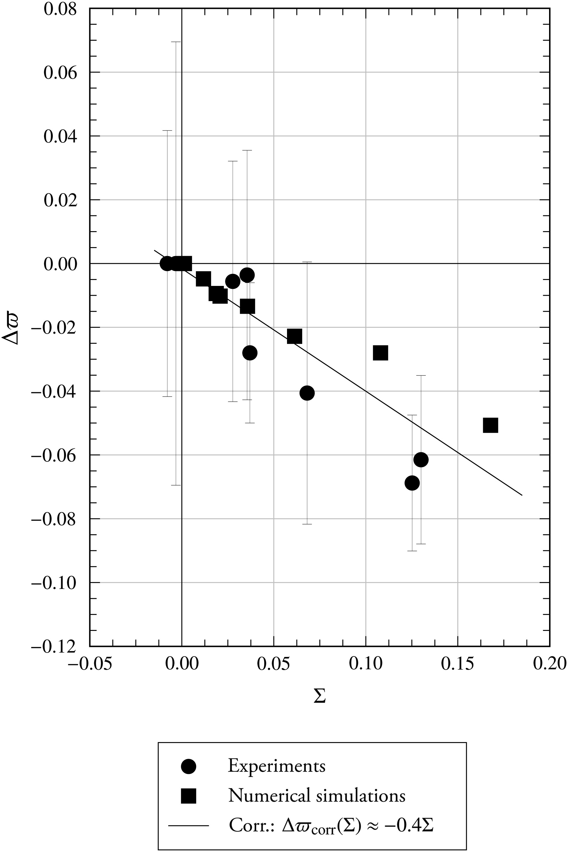
or, for a regression that goes through the point of origin
Since
Here, we introduce the loss rectification factor Λ to quantify the effect of wakes and other non-vortex-induced phenomena. For the rotor investigated, it is defined as
We suspect that the exact definition of Λ is dependent on the exact geometry of the rotor and may require additional rectification factors. Regardless, this requires further studies. While the correlation proposed in Equation (20) indicates a clear relation between total pressure losses generated in the diffuser and the degree of boundary layer stabilisation its physical underpinnings shall be further discussed.
Dissipation
As initially discussed, the dissipation terms of the energy equation and the enstrophy equation,
Unlike the term given for
shall be used in the following. In this formulation, the viscosity μ has been replaced by the sum of molecular and turbulent viscosity μ + μt to account for the influence of turbulence. Figure 8 shows the circumferentially averaged relative magnitude of
Figure 8.
Circumferentially averaged distribution of non-dimensional energy dissipation D e , t / D e , t , ref , avg
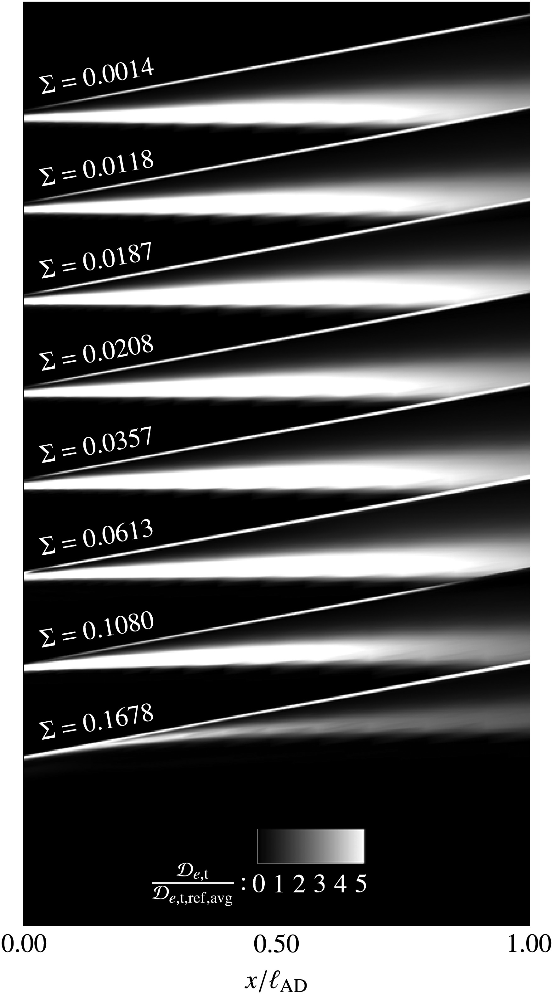
Apparently, the dissipation of energy decreases in intensity and expanse for increasing diffuser stability. This is consistent with the homogenisation of the velocity profiles seen in Figure 2. The five variants with the lowest stabilisation numbers (from bottom to top in Figure 8)—which are also located close to each other in Figure 6—are fairly similar, whereas a considerable weakening of the dissipation can be observed from Σ = 0.0613 to Σ = 0.1678.
Conversely, Figure 9 depicts the turbulent dissipation of enstrophy for different, representative operating points, that is,
Figure 9.
Meridional plane showing the time averaged distribution of non-dimensional enstrophy dissipation D E , t / D E , t , ref , avg
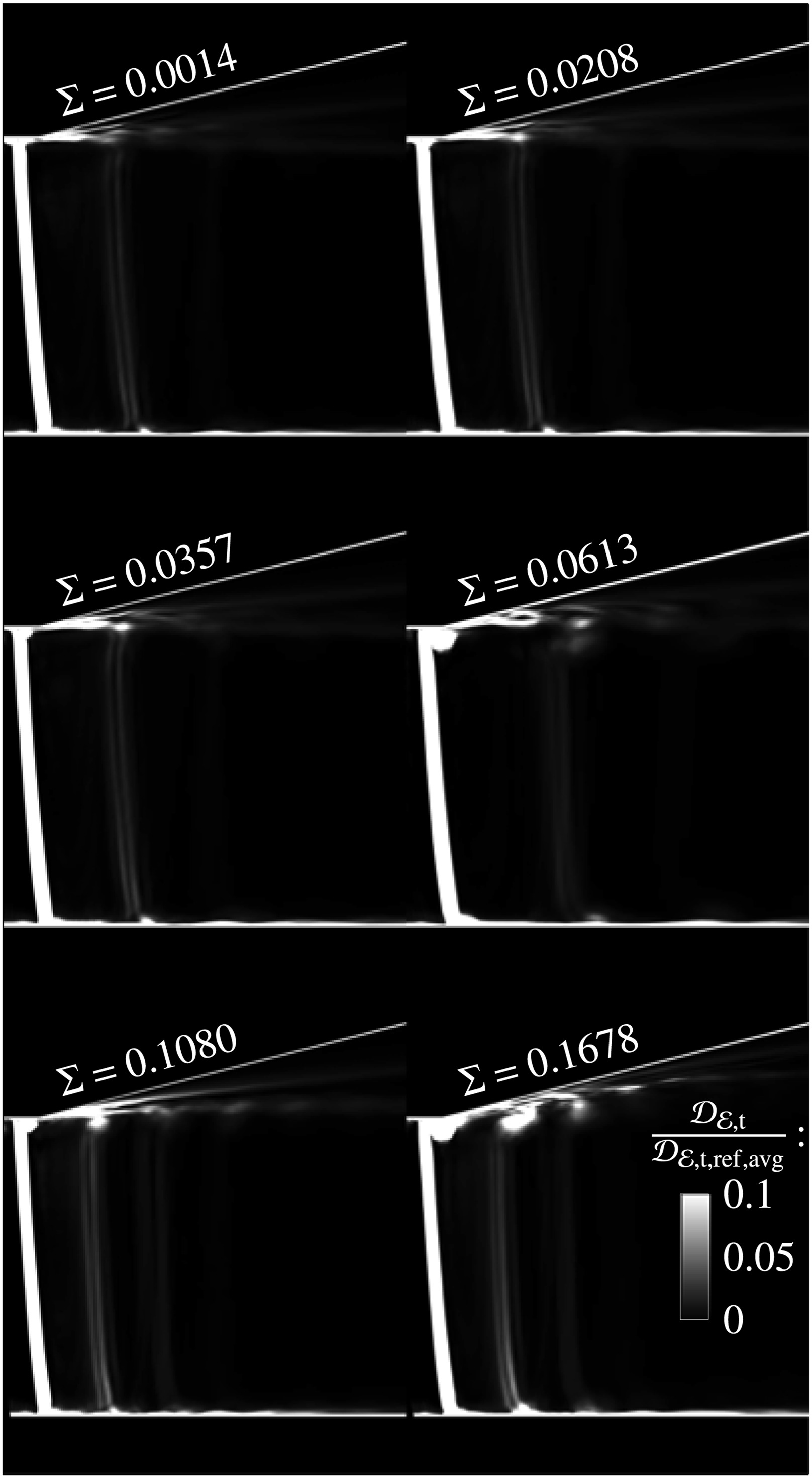
The contour plots are taken for meridional planes, which are oriented so that the trailing edge of the blade lies directly behind the plane. The slanted, white bar at the left of the individual figure frames is caused by the wakes and indicates the position of the trailing edge. One can see that the highly vortical tip leakage flow causes considerable enstrophy dissipation. An effect that becomes more accentuated for increasing values of Σ, as the tip leakage vortex becomes more powerful.
While the magnitudes of
Conclusions
The total pressure loss coefficient of the annular diffuser tends to decrease for growing stabilisation numbers. This is due to a more homogeneous radial flow profile stemming from pronounced interactions between the blade tip vortices and the boundary layer. The total pressure loss in the diffuser correlates well with the stabilisation number Σ, especially if wake mixing and swirl are accounted for in the form of a rectified total pressure loss coefficient
Therefore, we conclude that the results support the hypothesis initially stated—namely that the total pressure loss coefficient ζ decreases for increasing values of the stabilisation number Σ—if wake mixing and swirl-induced losses are accounted for.
We show that the loss mitigation is a consequence of the homogenisation of the boundary layer profile. This leads to smaller strain rates, which, in turn, reduces energy dissipation in the shroud near region of the diffuser. Even though dissipation of enstrophy contained in the wakes (which are accounted for, anyway) and the tip leakage vortices rises for growing values of Σ, this effect is locally confined and loses relative significance when unstable boundary layers and flow separations are present. Future research should emphasise further generalisation of the loss correlation presented. This includes studies on different diffuser opening angles, turbine-specific blade profiles, variations of the tip gap as well as DDES or LES of the influence of transition and flow separation happening on the blades or shocks in transonic low-pressure turbines.
Nomenclature
Unless otherwise noted only SI units are used.
Symbols
AR
area ratio of the diffuser
ci
flow velocity
cp
pressure recovery coefficient
dissipation
e
energy
ε
enstrophy
fbp
blade passing frequency
fred
reduced frequency
h
enthalpy (default: static)
height-wise coordinate
length
chord length
mass flow rate
n
blade count
N
rotational speed in revolutions per minute
p
pressure (default: static)
radius, Euler radius
R2
coefficient of determination
sij
traceless strain tensor
t
time
T
temperature (default: static)
u
rotational velocity
xi
generalised spatial coordinate
x
axial coordinate
α
flow angle, swirl angle
δ
diffuser half-opening angle
diffuser effectiveness
ζ
total pressure loss coefficient
circumferential coordinate
θ
single pitch
λ
thermal conductivity
Λ
loss rectification number
μ
dynamic viscosity
μt
turbulent eddy viscosity
ξ
kinetic energy coefficient
rectified total pressure loss coefficient
ρ
density
Σ
stabilisation number
Φ, Ψ
flow coefficient, loading coefficient
ω
vorticity