
Introduction
To reach climate goals, a social and political commitment is required to reduce carbon dioxide emissions. In the best-case scenario, CO2 emissions can be eliminated altogether. Other strategies to avoid the effects of greenhouse gas emissions include storing and recycling.
Two possible options are the Power-to-Methane concept (P2M) and the Carbon Capture and Storage concept (CCS). P2M concepts propose storing surplus renewable power through the methanization of H2 with recycled CO2 (Ghaib, 2017). In CCS processes, CO2 emitted from industrial combustion processes is separated, compressed, and then stored in geological strata (Lehner et al., 2012). To achieve large-scale reductions in CO2 emissions using the P2M and CCS concepts, compression of high CO2 and CH4 volume flows are required. Since radial compressors are not sufficient in such situations, axial compressors are needed.
Several studies have been conducted which have investigated non-conventional gases in turbomachinery. Among others, (Roberts and Sjolander, 2005) investigated the effects of the fluid properties on the aerodynamic performance of a geometrically non-adapted radial single-stage compressor, both experimentally and numerically. As a result, the isentropic exponent was revealed to be an important parameter in predicting pressure ratio, efficiency and choke mass flow. In part, empirical approaches, correlating the isentropic exponent with performance data, were compared to the experiments. In addition, (von Backstroem, 2008) dealt with the effects of the isentropic exponent on the performance of a geometrical non-adapted radial impeller for compressible flow, likewise making reference to the results of (Roberts and Sjolander, 2005). Von Backstroem presented an analytical method to scale the performance data of argon to carbon dioxide. His investigations showed a sole correlation of the isentropic exponent κ to the scaling of the density ratio. Under non-compliance of Mach number similarity, he reached the same gas performances. In contrast to (Roberts and Sjolander, 2005), the analysis carried out by (von Backstroem, 2008) indicated that the polytropic stage efficiency must be independent from the isentropic exponent.
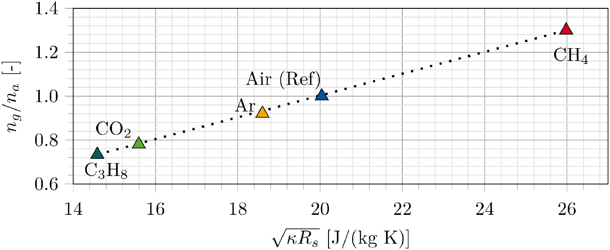
In contrast to the aforementioned studies, this paper deals with the effects of non-conventional gases in an axial compressor. While respecting the similarity of as many parameters as possible, to achieve a flow angle rematch not only a reference geometry is considered, but also a shroud adaptation applied. Multistage effects and global machine performance are evaluated both analytically and numerically. To analyse the aerodynamical influences, as well as the mismatch effects, four different gases (sorted by increasing isentropic exponent) are considered: propane (C3H8, κ = 1.13), carbon dioxide (CO2, κ = 1.29), methane (CH4, κ = 1.30) and argon (Ar, κ = 1.66). In addition to the processes for CO2 and CH4 previously mentioned, the monoatomic noble gas Ar and the polyatomic long chain hydrocarbon C3H8 are selected. With the wide range of isentropic exponents, which characterize the molecules’ degree of freedom, it is possible to gain a general understanding of mismatch and of the modifications which are required.
Similarity considerations
According to (Spurk, 1992), fluid mechanical equations with multiple parameters can be reduced to non-dimensional similarity parameters, defining the equation or problem with a reduced number of parameters.
For a given flow rate, the most important parameter characterizing the performance of a compressor is, under the constraint of preferable high efficiency, the total compression ratio Πt. To derive the dependent variables on Πt, the Euler equation provides a useful approach. An analysis of a common single compressor stage – rotor inlet, indexed by 1, and outlet by 2 – results in the following equation (adiabatic, calorically perfect gas)
(1)
Combining the two flow angles β1 and β2 in a single parameter β, the value of Πt is ultimately dependent on large extent on just five different parameters
Commonly used correlations in literature describing the Reynolds number effect have been summarized by (Wiesner, 1978). A simplified approach assumes that the total-total isentropic efficiency ηs,tt depends on the Reynolds number variation and a state of reference (ref)
According to (Wassell, 1968), the exponent n is an empirical value specific to each compressor. With respect to axial multistage compressors, (Schaeffler, 1980) collated multiple experimental results which showed a varying exponent between 0.1 and 0.15, later confirmed by (Grieb, 2009) for compressors in aircraft engines.
Using the Reynolds number correction approach according to Equation (3), the isentropic efficiency can be replaced by the inlet Reynolds number
The analysis of the stage pressure ratio underlines the importance of holding the inlet circumferential and axial Mach number, isentropic exponent, inlet Reynolds number and velocity triangles constant in order to satisfy Πt. So, in order to attain the same Πt for different working fluids in multistage compressors or to investigate the influence of certain parameters by keeping all others constant, it is necessary to first set these parameters to the same level as for the reference. However, this condition cannot be fulfilled. In part, the parameters can be adjusted to equal those for air. The isentropic exponent, in practical terms known as the ratio of specific heat capacity for constant pressure and constant volume, is a pure fluid property and not adaptable. A deviation in the pressure ratio is difficult to prevent, even though all other parameters will be set equal. Table 1 lists the parameters which define the OP and also specifies the adaptation.
Methodology
Compressor and adaptation constraints
The geometry investigated consists of the axial part of an axial/radial industrial compressor in a low-pressure section of an air separation plant. Disregarding the rear radial stage, the simulation model starts with an IGV and ends with an axial rotor, resulting in a quasi-eight-stage axial air compressor. The design point of air (reference) results in a total pressure ratio of Πt ≈ 2.2, with a volume flow of approximately 500,000 m3/h. With speed adjustments which enable Mach number equality at compressor inlet, it is possible to operate a compressor with non-conventional gases. However, the use of the non-adapted reference geometry will result to aerodynamical mismatch in downstream stages. To rematch the axial compressor stages for the design operating point (OP) with respect to air, downstream growth of unfavourable incidences should be avoided. In order to retain as many unchanged rotating parts as possible, only the shroud geometry is adapted.
Figure 1 describes this methodology, which ensures a rematch of the flow angles for the gases specified. Characteristic parameters are adapted, whilst taking into account the following constraints:
Numerical methodology
In order to examine the effect of different isentropic exponents and hence to get similarity in all other parameters specified in Table 1, iteration methods in conformity with the loops in Figure 2 are necessary. The axial Mach and Reynolds number at inlet can be set (loop I), as too can the flow coefficient φ (loop II). The circumferential Mach number is equalized by adapting the rotational speed at the inlet (not depicted in the diagram; see analytical approaches Equation 6).
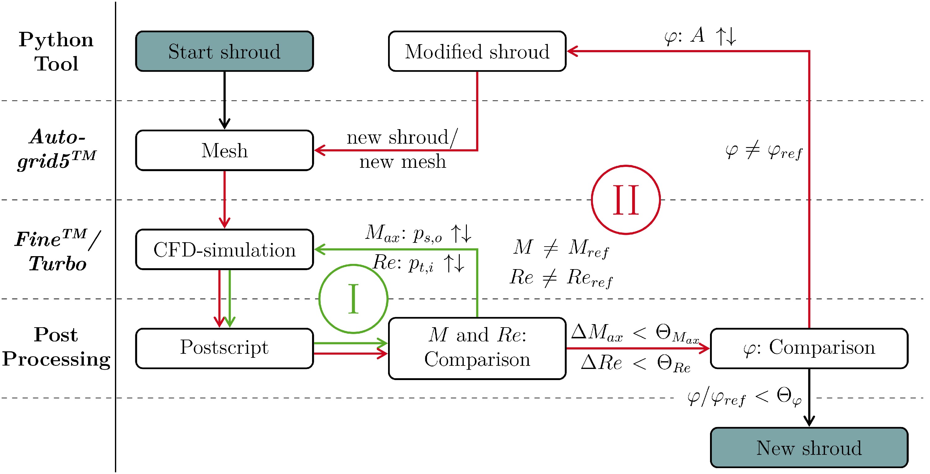
Loop I ensures the equalization of the axial inlet Mach and Reynolds number to the air reference. To set the required axial Mach number, the static outlet pressure is varied for each gas and for each new geometry. The Reynolds number is set by leveling the pressure. Factorizing the total inlet pressure and static outlet pressure only has an effect on the density. Due to the unmodified velocity and temperature field, the Mach number level is kept constant.
Loop II ensures the similarity of the velocity triangles in absolute blade span height. If the deviation in Mach and Reynolds numbers from the reference is smaller than the limit Θ, a comparison of the flow coefficient φ takes place locally. The post-processing routine evaluates 500 circumferentially averaged points in the mid-span section. If the local deviation is smaller than the limit Θφ, the new shroud geometry can be identified and the velocity triangles can be rematched.
If the limit Θφ is exceeded, loop II will start again. The cross-sectional area A is adapted by using the correlation in accordance with the continuity equation, evaluated for one gas type
The matched axial Mach number at the inlet ensures the same mass flow. Taking into consideration a blade span at a constant radius, the circumferential velocity is also kept constant. Assuming there are only small changes in density during geometry modification, it is possible to calculate the new cross-sectional area Anew with the deviation of the actual flow coefficient φact in relation to the target value of the reference φnew. By evaluating φ, a new shroud geometry can be generated. After meshing and simulating the new geometry under the constraints of loop I, the loop II starts again until all the limits Θ in Table 2 are reached.
Numerical settings
To model the axial compressor in stationary 3D CFD, the fluid domain is discretized by 27 million cells in AutoGrid5™. Constant radial gaps and fillets are used for the 16 rows. To achieve a y+ of approximately 1, the wall distance of the first cell is set to 1e-6 m. Even for C3H8, characterized by the highest Reynolds number in rear stages, the wall resolution adheres to the low Reynolds conditions.
For each gas, two simulations were conducted using the same reduced rotational speed. Firstly, using the air reference geometry to show the full aerodynamical mismatch; and secondly, by simulating an iterated shroud geometry to rematch the OP of the air reference.
The fluid is turbulently modeled with a turbulent viscosity of μtu = 0.0001 m2/s at inlet. To solve the stationary RANS equations and to model the turbulent content of the flow in FINE™/Turbo, the one-equation Spalart Almaras model according to (Spalart and Allmaras, 1992) and (Allmaras et al., 2012) is used. To combine rotating and stationary rows, a 1D-non-reflecting mixing plane interface is set. By combining the outlet static pressure with the inlet conditions for flow angle, total pressure, total temperature and turbulence, the modelled NSE can be iteratively solved.
The variation in heat capacity with rising temperature, especially for molecules with low isentropic exponents (e.g. long-chained hydrocarbons like propane), is taken into account by means of a one-dimensional heat capacity distribution over temperature (NUMECA real gas model). The ideal gas law is still valid by taking into account the effect of molecules’ frozen degrees of freedom. In this case - a temperature range of 300–450 K and pressure range of 0.5–2.5 bar - deviations from the ideal gas law model are negligible.
Results and discussion
Analytical approaches
Before examining the numerical approaches, analytical considerations are made. These introduce changes in compressor characteristics and thermodynamics, so that an understanding of the behavior of non-conventional gases can be gained. All the results relate to air as reference. For reasons of practicability, all derivations are made within the following constraints:
Geometry: Constant mid-span radii (rm,g = rm,a) and constant inlet cross-sectional area
Thermodynamics: Constant gas parameters (cp, Rs, κ), constant inlet parameters (pt,i, Tt,i), constant isentropic total-total efficiency (ηs,tt)
Aerodynamics: Similar velocity angles (equal flow angles)
Rotational speed
As a first step, the rotational speed for the different gases is deduced. In compliance with circumferential Mach number similarity for air (a) and a non-conventional gas (g) (Mu,i,a = Mu,i,g), the rotational compressor speed results in
Keeping the total inlet temperature and the inlet geometry constant for each gas, the ratio of the radii and the ratio of total temperature can be set to one. With the known inlet Mach number of the OP for air (Mi,a = Mi,g), the speed ratio can be calculated. With the given rotational speed of air of 3,000 rpm, it is possible to calculate the rotational speed for each gas (Table 3) using Equation (6).
Disregarding the small static temperature change in the speed of sound, the rotational speed is approximately linear, depending on
Total temperature
Having identified the rotational speed for each gas ng, the relative rise in specific enthalpy can be calculated. Firstly, the temperature rise in a single stage is considered. The total enthalpy ratio of a specific gas and air can link the velocity and the temperature field
(7)
Given the aim of rematching the flow angles of air and the restriction of unchanged blade geometry, the ideal similarity of velocity triangles can be assumed. The flow coefficient φ (φ = cm/u) and the flow angle alpha are therefore equal to the values of air
Using the linearity of the Equation (7), the total temperature rise of the compressor can be evaluated over the number of stages N
With the known total temperature rise of air
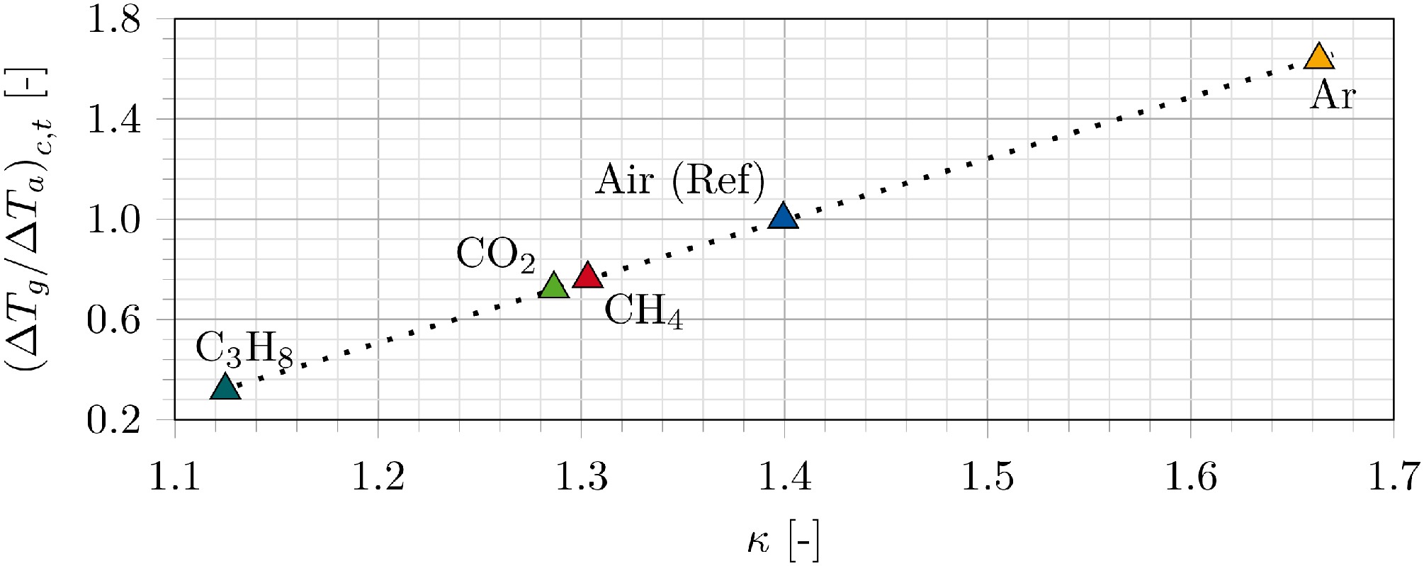
In Figure 4, the ratio of ΔTt,c,g/ΔTt,c,a is plotted against the isentropic exponent κ. The ratio of temperature rise occurs independently from deflection and stage loading. With the rotational speed calculated on the basis of Equation (6) and Table 3, the specific gas constant Rs in the product of Kgas and Kn is eliminated. It is possible to deduce an almost linear dependency on the isentropic exponent.
Pressure ratio
The total temperature rise ΔTt,c,g and the constant total inlet temperature Tt,i,g are used to calculate a new pressure ratio for the gases selected. The combination of the isentropic relation and the temperature rise leads to the total pressure ratio
An assumed constant isentropic total-total efficiency (ηs,tt,c,a = ηs,tt,c,g) results in an approximately linear dependency of Πt,c,g/Πt,c,a on the isentropic exponent κ (Figure 5).

With a minimum of −10% (C3H8) and a maximum up to +9% (Ar), the pressure ratio of air cannot be achieved, even though the flow angles are kept equal.
Changes in cross-sectional area
Using the aforementioned equations for total temperature (Equation 10) and total pressure rise (Equation 11), it is possible to calculate the change in cross-sectional area. Forming the ratio of circumferential Mach number of a gas and the reference leads to the following equation
By adapting the rotational speed, the Mach number is set to equal the Mach number of air at compressor inlet. An evaluation of Equation (12) reveals an inevitable Mach number mismatch. Figure 6 shows that the deviation in Mach number increases downstream of the compressor inlet.
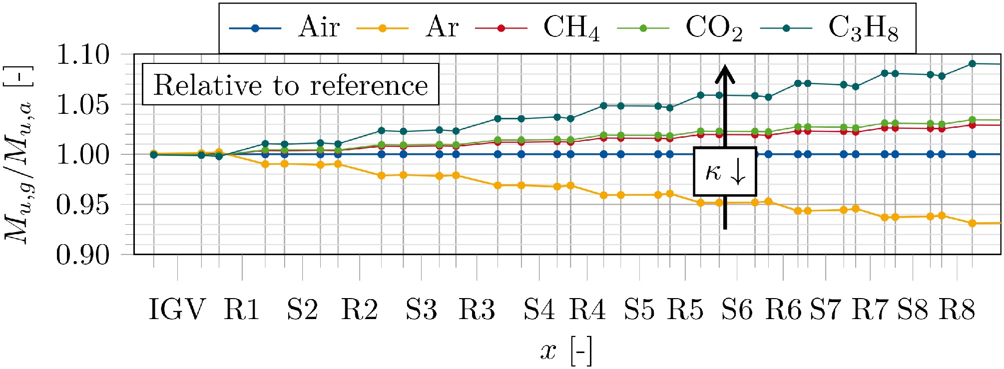
Due to a different rise in temperature, the analytical theory indicates a deviation in speed of sound, which depends on the isentropic exponent. Consequently, these differences cause a change in Mach number from −7% (Ar) up to 9% (C3H8).
According to the equations of total temperature rise (Equation 10), total pressure rise Equation 11) and change in Mach number (Equation 12), the thermodynamic deviation of the gases away from the reference state of air is known. Using the continuity equation an expression for the cross-sectional area can be derived
(13)
Equation (13) can be evaluated at every section downstream of the inlet (Figure 7), using the data of the reference simulation, given inlet boundaries and a constant isentropic total-total efficiency.
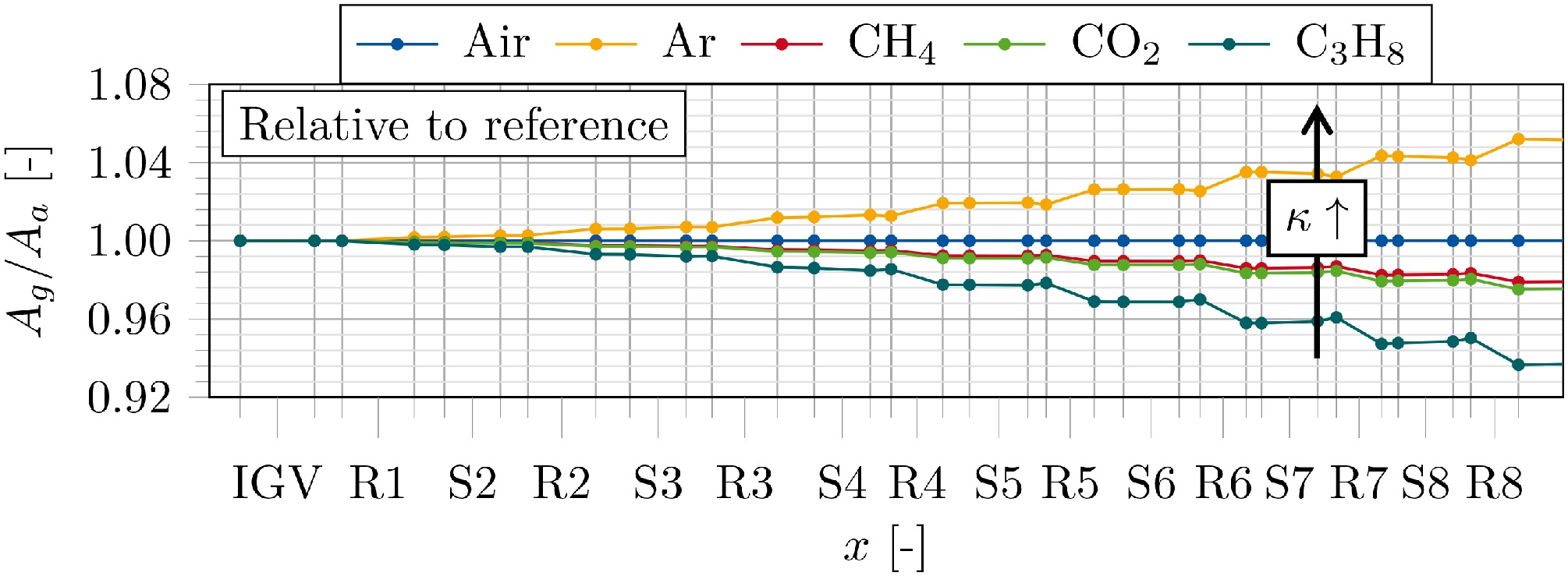
The deviation is staggered by the isentropic exponent κ. According to the simplified equations, the cross-sectional area has to be changed by up to −6.4% (Min.: C3H8, κ = 1.13) downstream of R8. In comparison to the reference annulus, the annulus cross-sectional area for gases with isentropic exponents greater than air has to be increased by up to 5.6% (Max.: Ar, κ = 1.66).
For summarizing the origin of deviation, the continuity equation can be considered. Due to the scaling of the velocity triangles with the speed ratio ng/na, the relative deviation of the meridional velocity of air remains constant downstream of inlet. But since the temperature and pressure distribution change, the relative density distribution also varies for each gas, correlating to the deviation of the isentropic exponent from air. The different gradients in density have to be compensated for by the cross-sectional area so that the same flow coefficients φ are achieved.
Numerical approaches
Numerical simulations were conducted to investigate the mismatch of the various gases using the reference annulus. In addition, the rematching of stages, employing an adapted shroud, is examined. For each simulation, the Mach and Reynolds number are adapted in conformity with Figure 2 (iteration limits: Table 2).
Non-adapted geometry
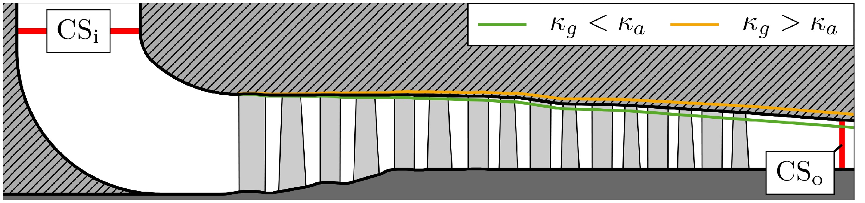
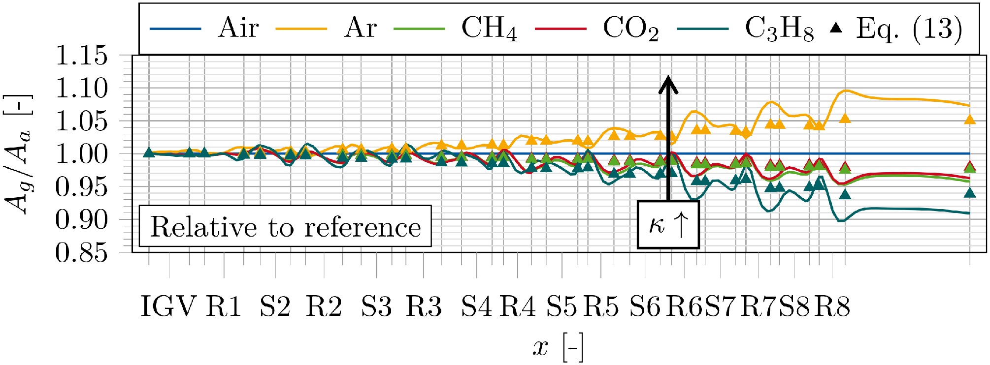
Figure 8 shows the relative deviation of the flow coefficient φ away from the reference simulation (air) for the circumferentially averaged mid-span section.
Figure 8.
Relative deviation of φ in mid-span section using the reference geometry (circumferentially averaged).
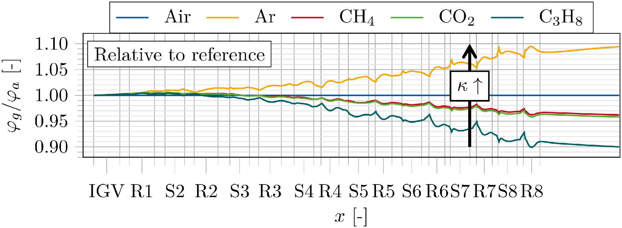
With increasing axial coordinate x and compression of the fluid, the deviation of φ increases. Staggered by the isentropic exponent κ, C3H8 indicates a deviation towards the lower end of −10% and Ar of up to +8%. In particular, in the rear second part, the reference annulus does not match the specific gas requirement for zero incidence to rematch the flow angles of air. As shown in Figure 7, the annulus size for κg > κa (e. g. Ar) is too small. The meridional velocity increases and the velocity triangles indicate a growing negative incidence. The OP for the rear stages shifts towards choke margin. The distributions for κg < κa (e. g. CO2, CH4, C3H8) indicate that the cross-sections become – staggered by κ – too large. The meridional velocity decreases continuously and positive incidence occurs in the rear stages. The OP of the rear stages shifts towards surge margin.
Taking into account the continuity equation with constant mass flow, constant mid-span radii and unchanged geometry, the product of φ and ρ also remains constant:
A changing flow coefficient φ therefore influences the density distribution and vice versa. Using the ideal gas law, the density rise can be attributed to static pressure and temperature rise. The numerics show that the gradient of the gas-dependent temperature rise has a greater influence on the compressor flow path than does the gradient of pressure rise.
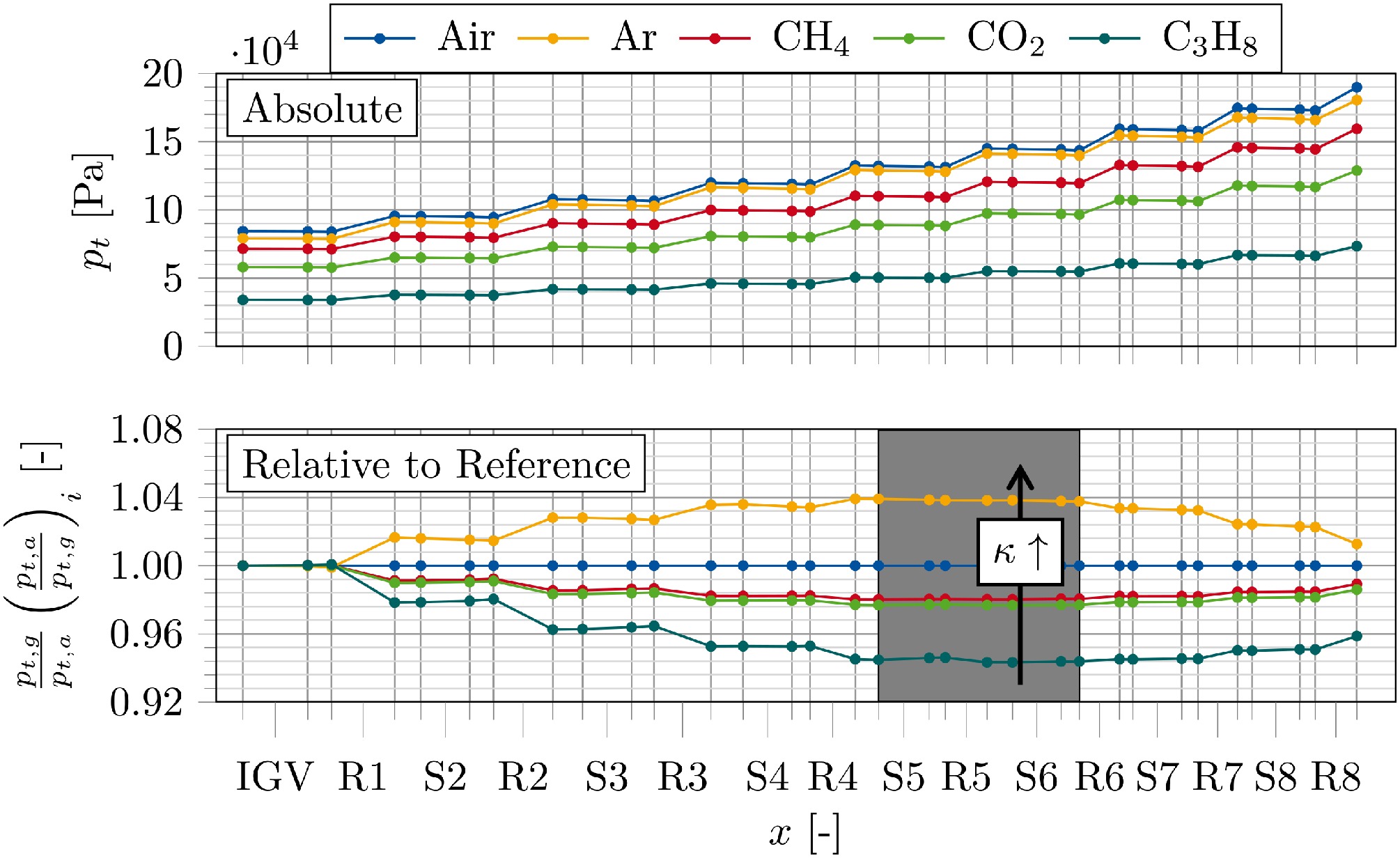
If the gradient of temperature rise is higher than that for air (e. g. Ar: κg > κa), the density increase will slow down. In conformity with Equation 14 and a constant product of φ and ρ, φ increases. The OP for the following stages shifts towards choke. Consequently, the pressure rise, depicted in Figure 9, is reduced. An inflection point occurs between stages 5 and 6 (marked area) and the relative gradient becomes negative (Figure 9, bottom). For the gases with κg < κa, the opposite effect occurs. Lower temperature gradients compared to the air reference result in an increase in density and growing positive incidence. The relative pressure gradient turns from negative to positive. The non-adapted shroud geometry does not ensure the same deflection for each gas. In rear stages especially, large incidence effects are indirectly attributable to the isentropic exponent.
The Mach number distribution shows the same trends. The circumferential Mach number depends mainly on the temperature rise and is therefore staggered by κ (Figure 10, top). The axial Mach number also reflects the incidence effects. The effect of the growing relative deviation of the meridional velocity away from the inlet condition determines the distribution in the rear part of the compressor (Figure 10, bottom).

In order to summarize the results for the non-adapted geometry, it can be stated that the adaptation of the aforementioned similarity parameters at the compressor inlet is not sufficient. Even though the reference shroud geometry of the first stages keeps deviations with respect to air on the small side, the distribution of data in the rear part of the compressor is determined by density changes. Incidence effects and OP shifts are unavoidable without a cross-sectional adaptation.
Adapted geometry
The shroud adaptation according to loop II (the diagram depicted in Figure 2) results in a new cross-sectional area distribution, as shown in Figure 11.
Compared to the analytical data (markers), the CFD results present the same trends in expansion or reduction for the cross-sectional area. In anticipation of the efficiency correction in Equation 18 (yet to be derived), the assumption of constant efficiency in Equation 11 leads to a deviation between analytics and the numerics. Furthermore, the numerical cross-sectional change turns out to have much higher gradients. In particular, in the passage flow of the rotors, the similar deflection results in a larger deviation away from the reference cross-section, increasing with coordinate x in the rear stages. If the continuity equation is taken into account, this can be explained by the following: The cross-sectional area A is dependent on the reciprocal value of the density ρ (assuming a constant gas-to-air ratio of meridional velocity)
Density changes in rotor passage flows increase in the rear rotors. Due to the increasing influence of the rise in relative temperature compared to the rise in relative pressure in the rear stages, the cross-sectional variation turns out to be larger according to Equation 15.
With respect to the evaluation of the flow coefficient for the adapted geometry, Figure 12 depicts the relative deviation of φg away from the reference φa (circumferentially averaged, mid-span section).
Figure 12.
Relative deviation of φ in mid-span section for the adapted shroud geometries (circumferentially averaged).
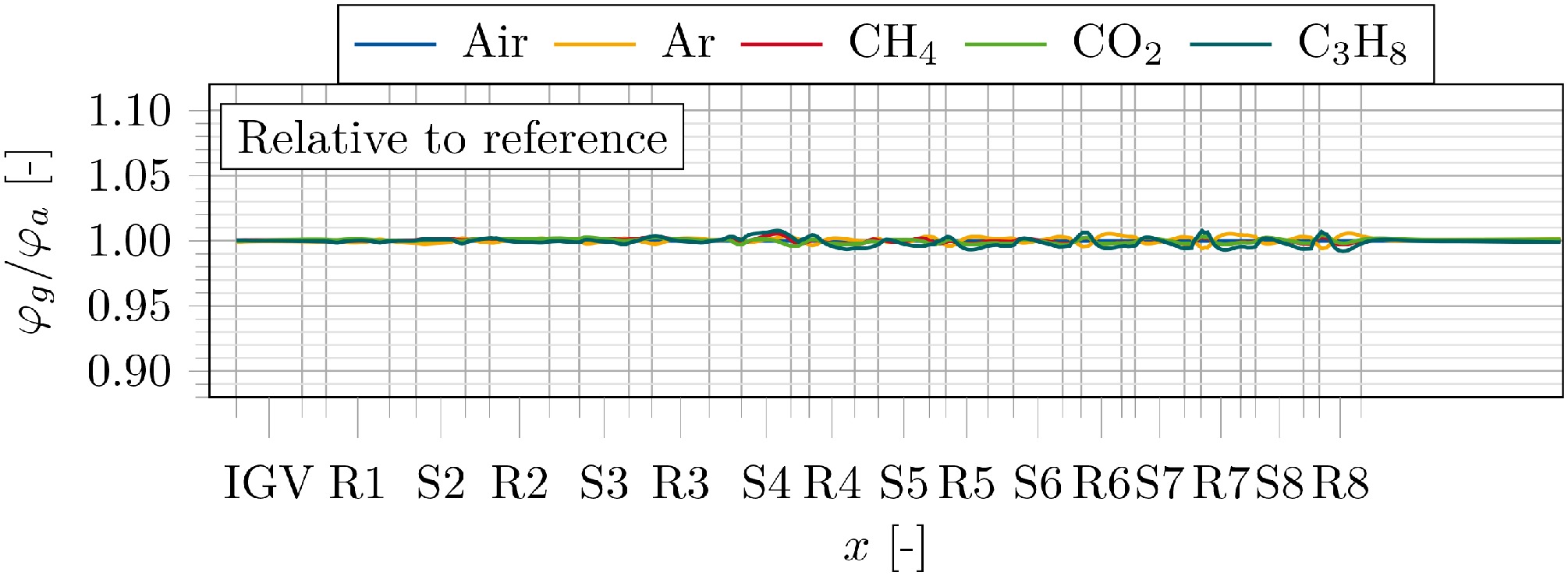
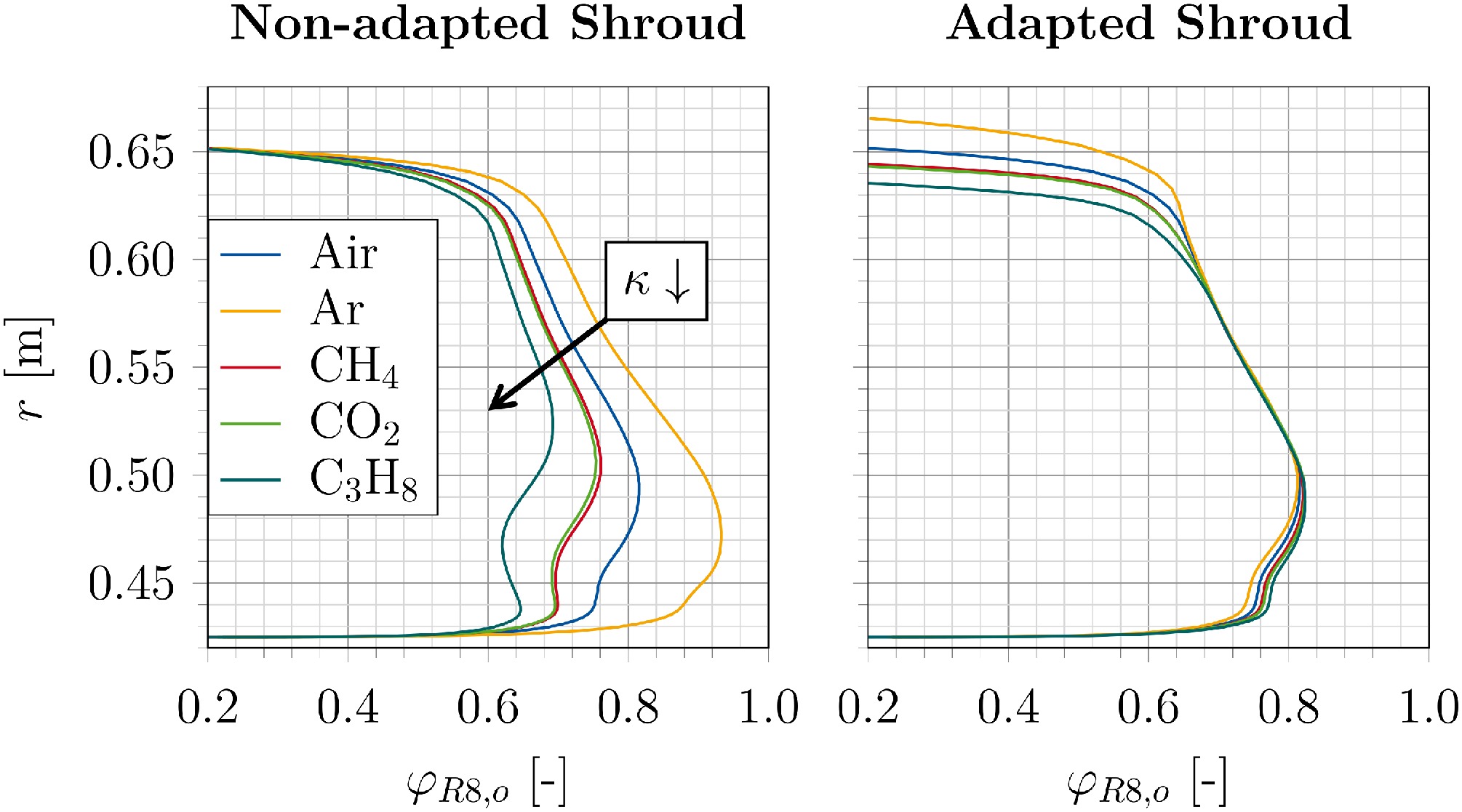
In contrast to the non-adapted geometry, the deviation of the flow coefficient diminishes to less than 0.8% compared to the previous 10%. The incidence is minimized. Also, radial distributions (circumferentially averaged) of φ show the alignment of velocity triangles. Figure 13 indicates the improvement downstream of rotor eight.
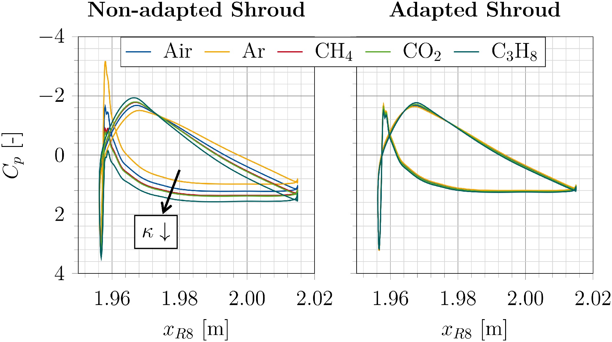
The necessary shift to rematch the air simulation aerodynamically can also be shown for the blade pressure distribution. The non-dimensional pressure coefficient Cp shows a general improvement and rematch for all rows.
Figure 14 shows the influence of the adaptation to R8 in the mid-span section. The aforementioned positive (Ar) and negative (CO2, CH4, C3H8) incidences, relative to the air distribution, are compensated for. The negative incidence flow is matched, which is typical for industrial compressors.
Comparing the temperature rise of the CFD results with the adapted shroud and the ideal analytics according to Equation 10, the conclusion can be made that the analytical approximation works reasonably effectively. A maximum deviation in temperature rise occurs for CH4 with +4% (≙ + 2.64 K). The expected small deviation in specific heat capacity for argon (monoatomic, noble gas) is approximated by the analytical model with constant heat capacity as the best among the gases investigated. That means that the smallest deviation in temperature rise is +0.25% (≙ + 0.37 K).
If the simulation with the reference annulus is taken into account, the difference in temperature rise is larger (up to 8 K for Ar). The incidence effects depicted in Figure 14 (left) cannot comply with the boundary conditions of similar velocity angles, required for analytics.
The performance data also confirms the approximate linear dependency on κ, already shown in the analytical part. Figure 15 depicts the change in total pressure ratio of the different working fluids against κ.
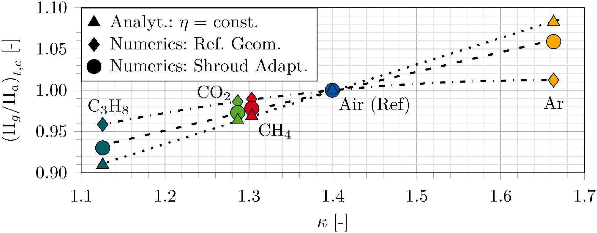
The numerically calculated pressure ratio of the gases deviates from the pressure ratio of air. Staggered by isentropic exponent, Ar (+5.9%) and C3H8 (−7.0%) diverge the most for the simulation with shroud adaptation. CO2 and CH4 have nearly the same pressure ratio, due to the same level of κ. When comparing analytical and numerical data, the analytics follow the trends, but do not reflect the CFD results exactly. A higher gradient in the trend line in Figure 15 leads to a larger deviation of the pressure ratio, up to an additional 2.3% (Ar) compared to the CFD.
The numerical results, conducted for the reference annulus (without shroud adaptation), show a smaller gradient. The incidence effects lead to a shift in the OP in the rear stages (as depicted in Figure 8), which reduces the deviation of the pressure ratio for each gas when compared to the results of the adapted geometry. The trend line (dash-dotted) shows a quadratic character. One reason for the differences in the pressure ratios between numerics with adapted shroud and analytics is the assumed constant efficiency in Equation 11. Figure 16 shows the deviation between the isentropic total-total efficiency ηs,tt,c,g of the numerics with the adapted shroud, which is staggered by κ, and the constant assumption of the efficiency for the analytics. The differences amount to up to +2.19% (C3H8) and −2.05% (Ar) for CFD. The data is similar to the pressure ratio in a linear dependency on κ.
Figure 16.
Relative change in isentropic total-total compressor efficiency for analytics and numerics against κ.

So far, the differences in efficiency cannot be assigned quantitatively to all causes and are still part of further investigation. Deviation in efficiency due to incidence effects is avoided. On the other hand however, the modified shroud geometries with accompanying different annulus heights induce a change in relative tip clearance and secondary flow characteristics. Furthermore, the thermodynamical behavior changes. Different Mach number levels in downstream stages, shown for each gas in Figures 6 and 10, influence compressibility effects, as well as changes in OP according to Equation 1.
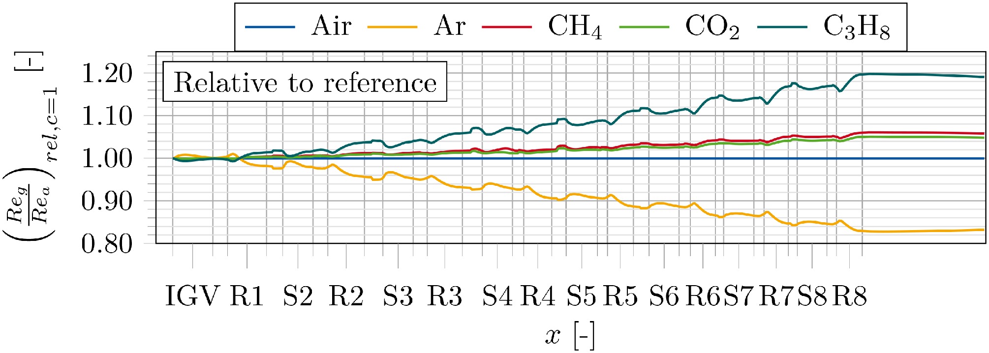
Even if the influences mentioned are difficult to separate and quantify from each other, one influence which can be highlighted here is the change in the Reynolds number and the related effect on efficiency deviation according to Equation 3. Figure 17 depicts the circumferentially averaged Reynolds number in the mid-span section of the compressor for each gas. Though the Reynolds number is equalized at the compressor inlet, Figure 17 indicates that the Reynolds number deviates downstream of the inlet up to 20% (C3H8) in rear stages. Similar to the Mach number and compressor efficiency, the Reynolds number decreases or increases with a higher or lower isentropic exponent respectively.
Figure 17.
Relative deviation of Reynolds number for the adapted shroud geometries (mid-span section).
Analyses can be deduced from the definition of the Reynolds number, converted by the ideal gas law and relative Mach number definition, to
Equation 16 shows a dependency of the Reynolds number on the parameters derived in the analytical part. The dynamic viscosity μ can be approximated using the Sutherland law (which is only a function of temperature), corresponding to (Sutherland, 1893) and for hydrocarbons to (Eakin and Ellington, 1963). Although μ is not a function of the isentropic exponent in general, the relative change of μ correlates - according to the analyses carried out - to the temperature rise and is therefore staggered by the isentropic exponent as well. The relative increase in viscosity of Ar is approximately 13.1% higher than the relative increase in air. This is in contrast to C3H8, for which the viscosity drops down to a relative −10.7%. All parameters in Equation 16 are attributed to κ. Equation 16 can be treated as roughly proportional to the isentropic exponent. The changes in Reynolds number, downstream of the inlet, can now be written as a simplified function of κ
So, at least the losses which correlate to the Reynolds number are an indirect function of the isentropic exponent and can be treated by Equation 3. Using typical exponents (n = 0.15) and the Reynolds number deviation (Figure 17) to evaluate Equation 3, the results show an underestimation in the efficiency deviation of only up to a relative 0.5% (Ar). Nevertheless, the overall isentropic total-total efficiency evaluated for the gases under investigation, depicted in Figure 16, shows a linear dependency. It should be noted that it is not only the losses affected by Reynolds number which are dependent on isentropic exponent, but the other aforementioned losses too. The overall change in isentropic efficiency can also be approximated using a new approach. Similar to Equation 3, a modified Reynolds number correction method is deduced. By correlating the inefficiency, not only in relation to the Reynolds number changes at the inlet, but also to the isentropic exponent, a new term can be conducted, representing the deviation of the isentropic exponent
As in some (experimental) cases, the distribution of the Reynolds number is not given. So the changes in the Reynolds number downstream of the inlet are referred to the deviation in the isentropic exponent. Similar to (Roberts and Sjolander, 2005), the fraction of isentropic exponent is attached to the fraction of the inlet Reynolds number.
The inlet Reynolds numbers for all gases compared are equalized and so the first ratio in Equation 18 is one and independent from exponent n. Similar to (Roberts and Sjolander, 2005) (m = 0.8) the exponent m is empirically set to 0.9 for this compressor case. According to Equation 16, the amount of change in Reynolds number downstream of the inlet, and hence part of the efficiency change, depends mainly on temperature rise (assuming a same level of efficiency). Due to the simple conversion of the reference temperature rise to the gas temperature rise according to Equation 10, the exponent m depends mainly on the reference temperature rise (here: ΔTt,c,a ≈ 90 K). The following function can be stated
With a higher temperature rise or compression, the Reynolds number change also increases and consequently the influence of κ on efficiency intensifies (m increases with temperature rise). To verify the assumption, more investigations need to be conducted, but so far the analytics are reasonable.
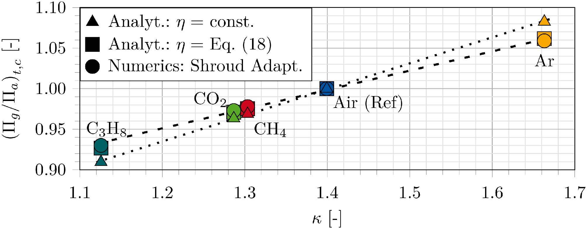
Figure 16 represents Equation 18 with m = 0.9 (black line). The analytical approach for the approximation of the isentropic total-total efficiency shows good agreement with the numerical results. Using the gas efficiencies, based on Equation 18, for a new calculation of the pressure ratio according to Equation 11, the differences to the CFD results with the adapted shroud geometry are reduced. Figure 18 shows these improvements for all gases. The semi-empirical approach for the correction of the efficiency according to Equation 18 reduces the deviation of the total pressure ratio estimation compared to the approach with assumed constant efficiency.
Compared with (Roberts and Sjolander, 2005), the difference is that the influence of the isentropic exponent is not directly attributed to the change in efficiency. Even though (Roberts and Sjolander, 2005) investigated a radial compressor and did not adapt the geometry, Figure 16 reveals that even the efficiency of a non-adapted geometry for an eight-stage axial compressor is influenced by analogous effects. Neither, for that matter, is the conclusion of (von Backstroem, 2008), entirely true, that is, that the stage efficiency of the single-stage radial compressor under investigation is independent from isentropic exponent. As has been shown for the Reynolds number deviation, the efficiency is directly or indirectly attributed to the change in isentropic exponent. Even though these calculations are based on an axial compressor, the analytics can most likely be reproduced for all other compressor cases, including multistage (larger effects) and single-stage (smaller effects) machines.
Conclusion
This paper presents analytical and numerical investigations showing aerodynamical effects and rematch methods for several gases in an eight-stage axial air compressor.
Firstly, analytical approaches based on similarity considerations were adopted. As a result of these, the isentropic exponent was revealed to be the most important parameter for the deviation of thermodynamical characteristics, such as temperature rise and pressure ratio. Consequently, derivations showed that the change in the cross-sectional area also depends on the isentropic exponent.
Secondly, 3D-CFD simulations were performed to verify and quantify the analytics. The gases Ar, CO2, CH4 and C3H8 were assessed in relation to the reference of air. In order to avoid downstream increasing incidences, as shown for rear stages of the reference geometry, a method was investigated whereby the shroud was adapted and the flow angles of air were rematched. The size of the shroud adaptation and the corresponding numerical results confirmed the analytical approximate linear dependence on κ. The more/less the isentropic exponents deviated from that of air, the higher/lower the rise in temperature, the pressure ratio and the change in cross-sectional area in the rear stages. In contrast to the assumed constant efficiency in analytics, the numerics also displayed a linear dependence of the isentropic efficiency on isentropic exponent. Analyses proved the indirect dependence of κ on the Reynolds number deviation downstream of the equalized inlet conditions. An empirical approach for correction of the efficiency was adopted using the ratio of gas and reference (air) isentropic exponent exponentiated with m = 0.9. The good concordance of the approximation of the CFD efficiency consequently leads to an improved calculation of the analytical pressure ratio.
All in all, this paper demonstrates analytically derived and numerically verified adaptation methods and inevitable mismatch prediction for non-conventional gases in an axial compressor. Even though the investigations were exclusively numerical in nature and require further experimental validation, the correlations provide reliable performance predictions and redesign methods for axial compressor used for gas processes like CCS and P2M.
Nomenclature
Roman letters
A
area
c
blade chord length
cp
heat capacity (constant pressure)
Cp
pressure coefficient
cv
heat capacity (constant volume)
h
enthalpy
i
incidence
K1
Mach number constant
K2
Mach number constant inlet
Kgas
constant (for each gas)
Kn
speed constant (for each gas)
mass flow
M
Mach number
m
exponent κ correction
n
exponent Re correction
n
rotational speed
n*
exponent Re correction inlet state
N
number of stages
p
pressure
r
radial coordinate
Rs
specific gas constant
Re
Reynolds number
T
temperature
u
circumferential speed
w
relative velocity
x
axial coordinate