
Introduction
The axial spacing between moving and stationary rows has been a major focus of research over the past years. This trend is driven by the need to optimize unsteady blade-row interaction and meeting design goals such as more compact components and reduced weight.
The axial-gap size affects the intensity of intra-row secondary flow, wake and potential interactions. Pressure fluctuations between moving and stationary rows can be subdivided into a uniformly steady component, a steady component relative to the reference frame of the stator and a steady component relative to the reference frame of the rotor. According to Jung (2000), the component which is steady relative to one frame acts as an unsteady fluctuation relative to the other component.
Praisner et al. (2006) argued that a larger axial gap would be beneficial regarding system loss, as the wakes mix out to a higher degree before they are affected by dilation resulting in higher loss. The wake impinging upon the leading edge of a downstream blade can result in increased incidence and can induce bypass transition, see, e.g., Coull and Hodson (2011); the intensity of both effects is inversely proportional to the axial-gap size.
For three-dimensional flow, however, secondary flow caused by the end-wall boundary layers has to be considered as well. As a result of the losses induced by secondary-flow vortices, as described by, e.g., Denton (1993), smaller axial gaps appear beneficial in this regard.
At the mid-span, Pichler et al. (2017) were able to identify higher losses for smaller axial gaps using quasi three-dimensional LES simulations. Because of decreasing potential-field-interaction effects and resulting lower wake dilation, the production of turbulent kinetic energy decreases, thus confirming the arguments of Praisner et al. (2006).
For a shrouded rotor with an aspect ratio of
In the studies conducted by Restemeier et al. (2013) and Gaetani et al. (2010), secondary-flow intensity was the dominant factor driving system loss. Both of the turbines investigated feature comparatively small aspect ratios and an unshrouded design, resulting in higher secondary-flow losses compared to profile losses. An optimum was found at a gap equal to 50% of the stator axial chord. Similarly, Park et al. (2003) observed higher efficiency for a smaller axial gap due to the decreasing intensity of secondary flow.
While the basic aspects of the axial-gap size effect – end-wall losses tend to increase with gap size, while profile losses typically decrease – are generally well-understood, a strong disagreement regarding the influence of axial-gap size on the total system loss can be identified in the literature. One reason for conflicting results is the general interdependency of the loss contributions as well as the axial-gap size effect correlating with secondary design parameters. Bellucci et al. (2017) found a strong interdependency of axial-gap-related losses with both aspect ratio and inlet Reynolds number. In a review of the literature, Grönman et al. (2014) were able to correlate the axial-gap size effect with secondary design parameters like the pitch-to-axial-chord ratio of the stator, circumferential Mach number, and the rotor aspect ratio. Additional dependencies, such as the rotor being shrouded or unshrouded, cavity design or blade loading, are likely to exist as well. Transonic flow and the presence of shock waves strongly affects loss generation and its dependency on gap size too (Venable et al. 1999).
Utilizing both experimental data and numerical results obtained from unsteady RANS calculations, this paper aims to show the development and sources of loss for three different axial gaps. Accounting separately for individual loss contributions in a quantitative manner forms the basis for future investigations into the interdependency of the axial-gap size effect with other design parameters and operating conditions. To this end, the present paper will answer the following three questions:
How does the total loss relate to the axial gap?
How do individual loss contributions depend on gap size?
What are the underlying physical effects?
Loss analysis
The most accurate and robust method to quantify loss is the assessment of the total amount of entropy present in a thermodynamic system.
Since the system considered is modeled using adiabatic wall boundaries, entropy as per
lends itself as the base quantifier of flow losses. In order to distinguish the losses according to their generating flow phenomena, distinct quantities for identification are needed. The distinction between different sources of entropy is based purely on phenomenological criteria and not on physical entropy-generating mechanisms, i.e., the losses are distributed amongst profile boundary layers, wakes, end-wall boundary layers (hub and tip), and secondary flow.
A common feature which all these flow phenomena share, is that they exist in flow regions where the vorticity
which is the projection of the vorticity vector onto the local velocity vector. Using the Pythagorean Theorem, the vorticity vector can be decomposed into a streamwise and a crosswise component perpendicular to the local flow direction
The crosswise vorticity is characteristic for boundary layers, wakes, and rotational shear layers in general. Based upon these considerations, the following blending factors can be formulated:
and
The subdivision between boundary layers on the end wall or profile and wakes, however, necessitates additional blending factors. To discriminate between end-wall and profile boundary layers or wakes, the vorticity in cylindrical coordinates
Here,
and
for a deviating orientation of the vorticity vector.
To further isolate the profile boundary layers from the wakes, a distinction is made, based upon the distance normal to the profile
The critical distance of
Regions, where
and
The regions between
The individual contributions to the overall entropy are, therefore, defined as follows:
The contribution of the secondary flow is given by
the profile boundary layer by
the hub boundary layer by
the tip boundary layer by
and the contribution of the wakes is determined by
Each individual loss contribution is then integrated over the main flow domain, i.e., the turbine excluding the cavities, to obtain the resulting total,
The approach shown here is also used to assess the loss contribution of shock-wave vortex interaction in Mimic et al. (2019) where it is found to produce similarly satisfactory results.
Test case
The general flow field of the present 1.5-stage turbine configuration was investigated previously by Henke et al. (2016) and Biester et al. (2013). A primary goal of this turbine design was to ensure a homogeneous flow field in the mid-span unaffected by the end walls. It is therefore suitable for quantifying losses according to the decomposition above.
Turbine configuration
The turbine is a low-pressure turbine with an aspect ratio of
Table 1.
Test conditions and stage characteristics
Detailed aerodynamic characteristics and a base verification of the overall time-averaged flow field can also be found in Henke et al. (2016).
Instrumentation
The instrumentation of the experimental setup has been devised in order to answer the questions posed in the introduction of this paper in terms of time-accurate and time-averaged measurements of the local flow conditions.
To quantify the overall efficiency, rake probes measuring total pressure and total temperature at the inlet and outlet as well as pressure instrumentation on the blade surfaces were designed during a numerical pre-test analysis, including a local optimization of measurement positions.
Figure 1 shows a sectional view of the flow path including the measurement planes (MP). MP00, which is located further upstream of the control volume and thus not shown here, features equally spaced rake probes to verify the homogeneous, swirl free inlet flow of the turbine on a grid of six circumferential rakes with six radial positions each. Rake probes in MP32 have been designed to deliver a 360 deg record of total quantities as well as the static pressure and swirl angle. In order to operate these rakes in the three-dimensional flow field downstream of stator 2, the kiel-head probes have been designed with a pre-twist in order to record accurate data of the local flow-field for all radial measurement positions.
Figure 1.
Schematic of the 1.5-stage turbine test rig. Small gap X / C ax = 20 % X / C ax = 80 %

As these rake probes provide only limited radial resolution of the flow field, additional five-hole-probe measurements have been conducted in the measurement planes MP10 (inlet section) and MP31 (outlet section). While rake probes allow continuous data acquisition, probe traverses provide better resolution in radial direction for a specific point in time. A combination of these data sources provides a set of high-resolution boundary conditions for each experiment, which are used in the present work. Within the stator-rotor and rotor-stator gap regions between the blade rows, time-averaged as well as time-resolved multi-hole-probe traverses were conducted for the medium and large axial-gap configuration. For the smallest gap investigated, the remaining gap between two blade rows is too small for probe measurements. Therefore, the blading itself has been equipped with pressure taps (time-averaged and time-accurate wall taps) on the suction and pressure sides and in the leading and trailing edges. This allows determining the wake-flow properties and unsteady flow characteristics for all three axial-gap configurations.
Numerical setup
The experimental data is supplemented by steady and unsteady RANS calculations for all three gaps using the TRACE solver, which is being developed by the German Aerospace Center (DLR) in cooperation with MTU Aero Engines AG. The general numerical setup used in this work is mostly identical to the ones described by Henke et al. (2016) and Biester et al. (2012). The following short summary will focus on modifications to the referenced setups.
For steady-state calculations, mixing planes are positioned at 50% of the axial gap. For unsteady simulations, one blade passing period (BPP) is resolved by 192 time steps; each time step is resolved using 30 sub-iterations. A Courant-Friedrichs-Levy
To assess convergence, the fluctuating pressure signal at several point probes inside the computational domain is evaluated. Convergence is reached when the maximum amplitude deviation between two periods is below a threshold of
Flow field analysis
In line with the introductory discussion, the flow field is decomposed into a quasi-two-dimensional flow at the mid-span and three-dimensional flow across the entire span. In order to obtain a better understanding of the loss evolution, axial distributions are considered as well.
Axial distributions
Figure 2 depicts the axial distribution of the circumferentially and spanwise-averaged entropy for all gaps. Four regions of interest are identified:
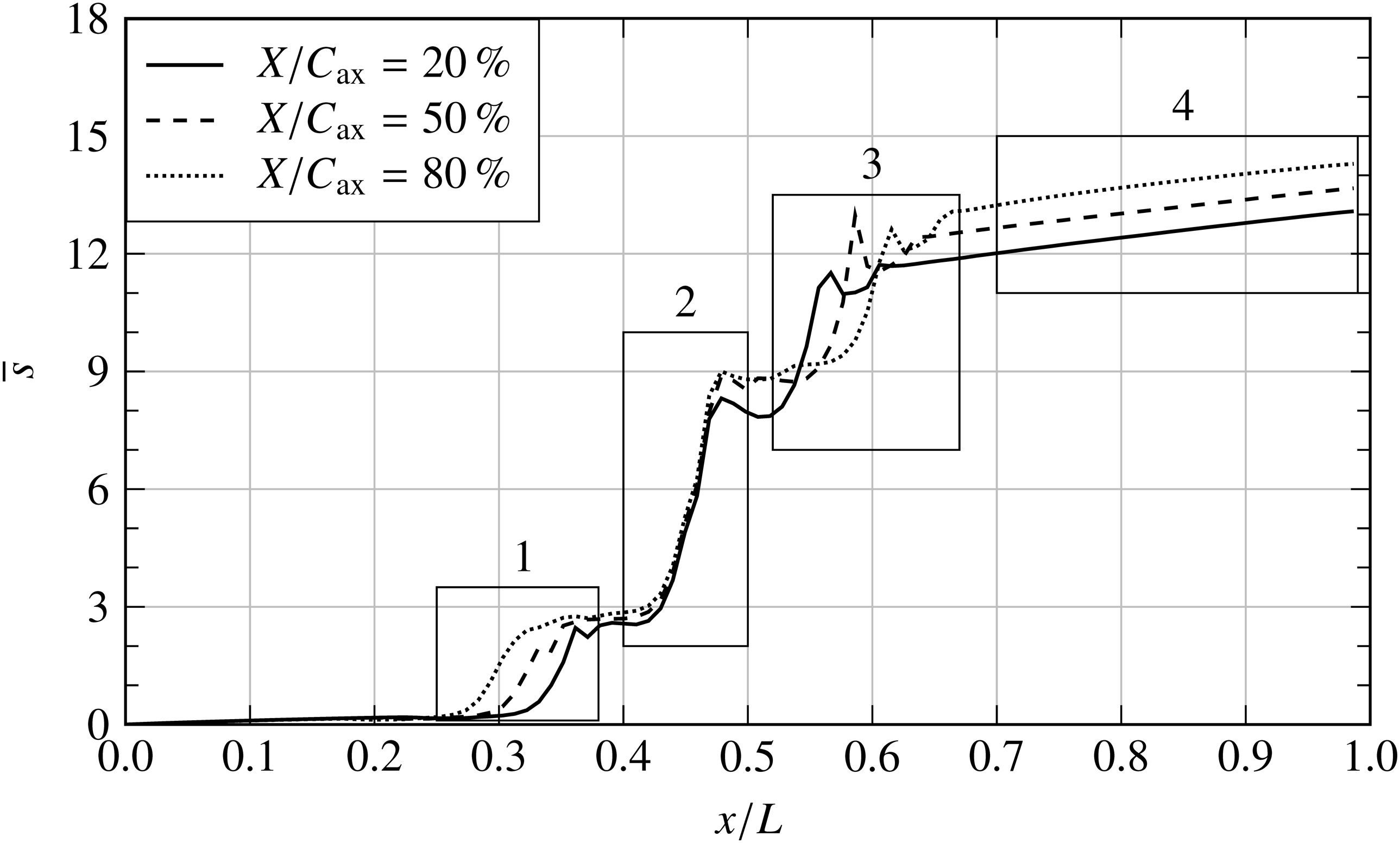
Stator 1: Losses are initially proportional to the flow path length upstream of the stator 1 leading edge. Downstream of the first stator, losses increase initially for larger axial gaps as a result of increased secondary-flow and wake-mixing losses.
Rotor: All axial gaps show a nearly identical slope in entropy increase. For the smallest gap, total losses at the rotor trailing edge are substantially lower than for the other gaps.
Stator 2: Due to the stronger wake-boundary-layer interaction at the second stator, losses increase for the smaller gaps.
Flow downstream of stator 2: Wakes and vortices mix out increasingly, resulting in linearly increasing losses. The slope is flat relative to the absolute difference between axial gaps, i.e., compensating smaller axial gaps with an outlet further upstream – as would be the case for neighboring components in a real machine – does not result in equal total system loss.
Since cavities are not included in the post-processing control volume, entropy fluctuations at the cavity inlets and outlets can be observed, which can also result in a local entropy decrease in the main flow domain. Generally speaking, the entropy increase is steepest in the rotor and stator passages, whereas it is less pronounced outside of the blading. Minimum system loss occurs for the smallest axial gap, while the losses are highest for the largest gap examined. The underlying physical effects are investigated below in further detail.
Two-dimensional flow field
For the quasi two-dimensional flow field at the mid-span, profile losses are the dominant factor. Instantaneous entropy contours at different time steps are pictured in Figure 3 to visualize the wakes for the small and large gaps. The low-momentum wakes of the first stator enter the rotor, experience dilation and are transported into the second stator frame. Because of the comparatively high turning, an increase in axial gap affects the wake mixing process disproportionately. For the large axial gap, the wake is almost entirely mixed out when entering the rotor, the same is true for the rotor wakes entering the second stator. For the small gap, wakes are deflected by the leading edge of the downstream row almost as soon as they are shed: A strong interaction of the wake with the potential field of the downstream row can be inferred. Downstream of the second stator, a highly unsteady flow field can be identified, which is caused by the comparatively strong wake-inducing periodic fluctuations on the suction side: Wakes of varying intensity are shed. As a result, entropy production at the mid-span increases considerably for the smallest axial gap. This evaluation is consistent with the two-dimensional prediction of Praisner et al. (2006).

Three-dimensional flow field
The essential aspects of the three-dimensional flow field in the form of circumferentially averaged flow variables were presented by Henke et al. (2016). Figure 4 depicts distributions of streamwise vorticity in measurement plane (MP) 12. With the distance between rotor trailing edge and MP12 remaining constant despite gap variation, both gaps show only minor differences regarding secondary flow, represented here by the streamwise vorticity and the streamwise loss component
Figure 4.
Time-averaged flow field downstream of the rotor (MP12, URANS). Dash-dotted lines denote sCW; solid lines sSW.
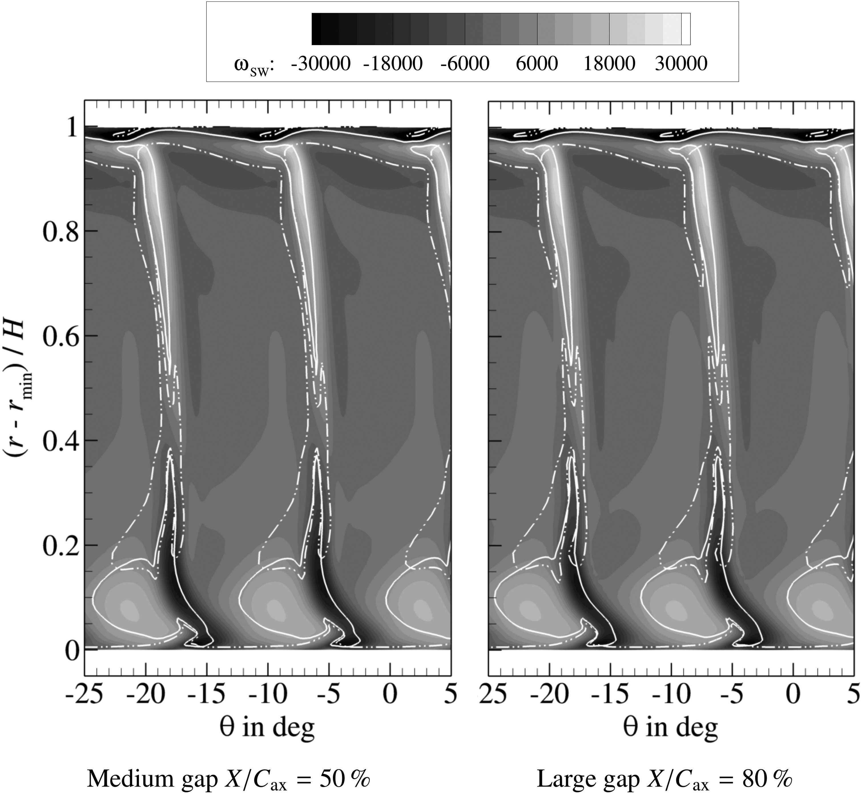
Figure 5 depicts the distribution of the circumferentially averaged streamwise vorticity downstream of the second stator. Additionally, a single contour line of the loss contribution
Figure 5.
Circumferentially and time-averaged streamwise vorticity downstream of stator 2 featuring loss contribution sCW,⌝r (URANS).
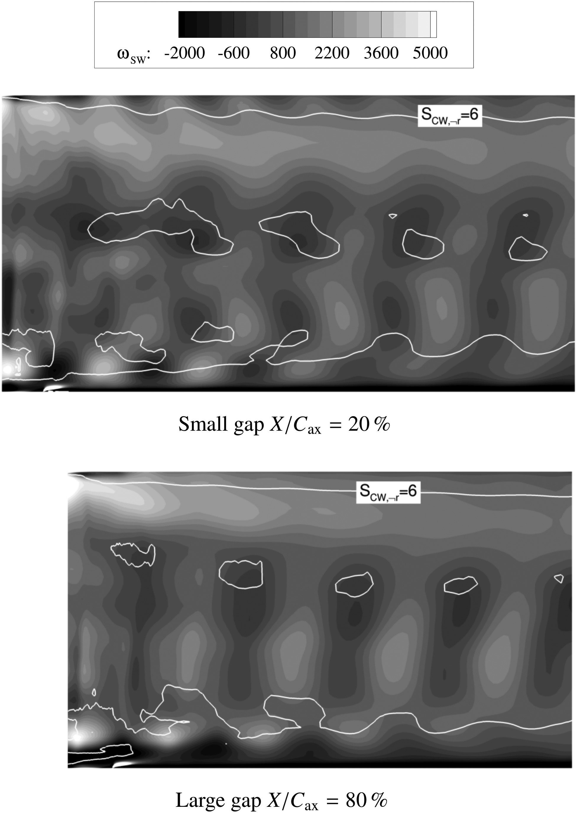
Additional spots of increased
Integral parameters
Loss analysis
Based upon the detailed flow analysis, losses are broken down in Figure 6. The present study shows that the total system loss increases with the axial-gap size. These results are consistent with Yamada et al. (2009), who investigated a similar turbine configuration. In the hub and tip regions, more pronounced boundary and shear layers from the cavity interaction increase losses for larger gaps. As is evident in Figure 5, the end-wall losses at the hub are higher than at the tip which is also reflected in Figure 6. The profile losses, i.e., the losses immediately caused by the blade boundary layers, are a negligible loss factor and remain almost constant regardless of the axial gap. Interestingly, wake losses also show little variation for a change in axial-gap size. As can be seen in the efficiency distribution in Figure 7, a greater flow-path length between the stator 2 trailing edge and the outlet – which results from a decrease in axial-gap size – leads to an increasing redistribution of total enthalpy from the mid-span into the end-wall regions. This effect is superposed by the aforementioned merging of the end-wall boundary layer and wake structures. Since wake-torsion losses are only accounted for between 15% and 90% of the channel height, as per the definition above, a redistribution into the boundary layers results in an underestimation of the wake-induced losses, i.e., wake losses are counted as end-wall losses in the loss decomposition proposed. This is due to the end-wall and wake-torsion losses being both represented by
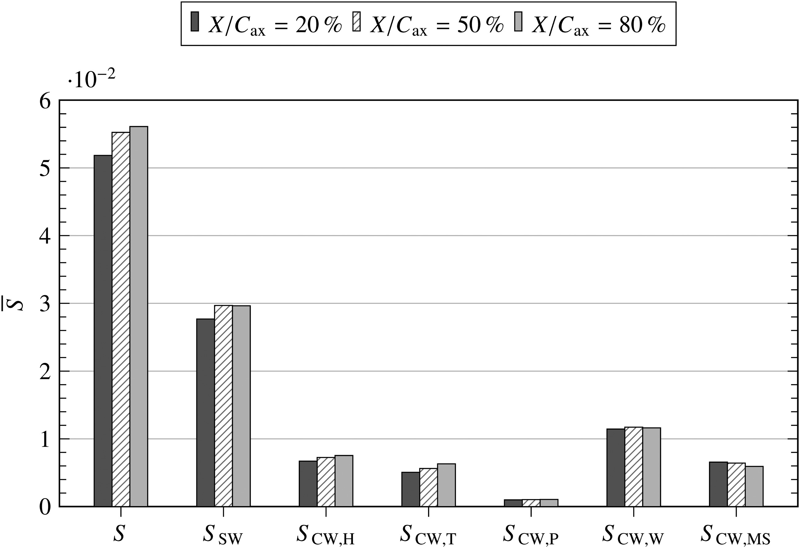

The losses observed in the mid-span region can be subdivided into direct wake-blade interaction, mixing losses and wake torsion with resulting vortex deflection downstream of the blades. As shown in Figure 3, the maximum increase in entropy actually occurs downstream of stator 2 and not inside of the blade passages, leading to the conclusion that the latter two effects are dominant with regard to wake losses.
The nearly identical secondary-flow losses for the medium and large axial gap suggest that the small axial gap inhibits the formation of secondary-flow-vortex structures disproportionally. If the gap reaches a certain threshold, the secondary-flow losses remain mostly constant, the effect of the increased flow-path length is reflected in the end-wall boundary layer losses. Considering Figure 5 and the decomposition above, it can be argued that the increase in secondary-flow losses occurs primarily in the tip region downstream of the second stator. For the investigated aspect ratio and operating conditions, end-wall related losses (secondary flow and end-wall boundary layers) account for roughly 2/3 of the total losses.
System efficiency
Figure 7 depicts the flow field at the outlet of the control volume for all axial gaps investigated. Of note is the missing total-pressure measurement at 93% of the channel height for the large gap. As the total-pressure information is missing for 2 circumferential positions, no representative average can be calculated at this position. Because of this, and a similar error for the total temperature measurement at 9% of the channel height, no efficiency information at these positions can be given for the large-gap case. For the isentropic efficiency, a clear distinction of the axial-gap size effect depending on radial location can be identified in accordance with the loss breakdown presented: In the hub and tip regions, losses increase for larger gaps. While the hub region shows higher losses in general, the variation, i.e., the influence of the axial-gap size, is higher in the tip region than at the hub. In the region between 40% and 70% of the channel height an inverse trend can be identified, i.e., losses increase for smaller gaps. Of particular note is the aforementioned redistribution from the mid-span region towards the end-wall regions. The small-gap distributions are, therefore, more uniform compared to the larger gaps. The trends discussed apply to both numerical and experimental data although different predictive trends exist at some radial positions. While the good agreement in the total pressure distribution validates the loss breakdown above, the comparatively high measurement uncertainty, however, precludes a detailed assessment of the experimental efficiency distribution.
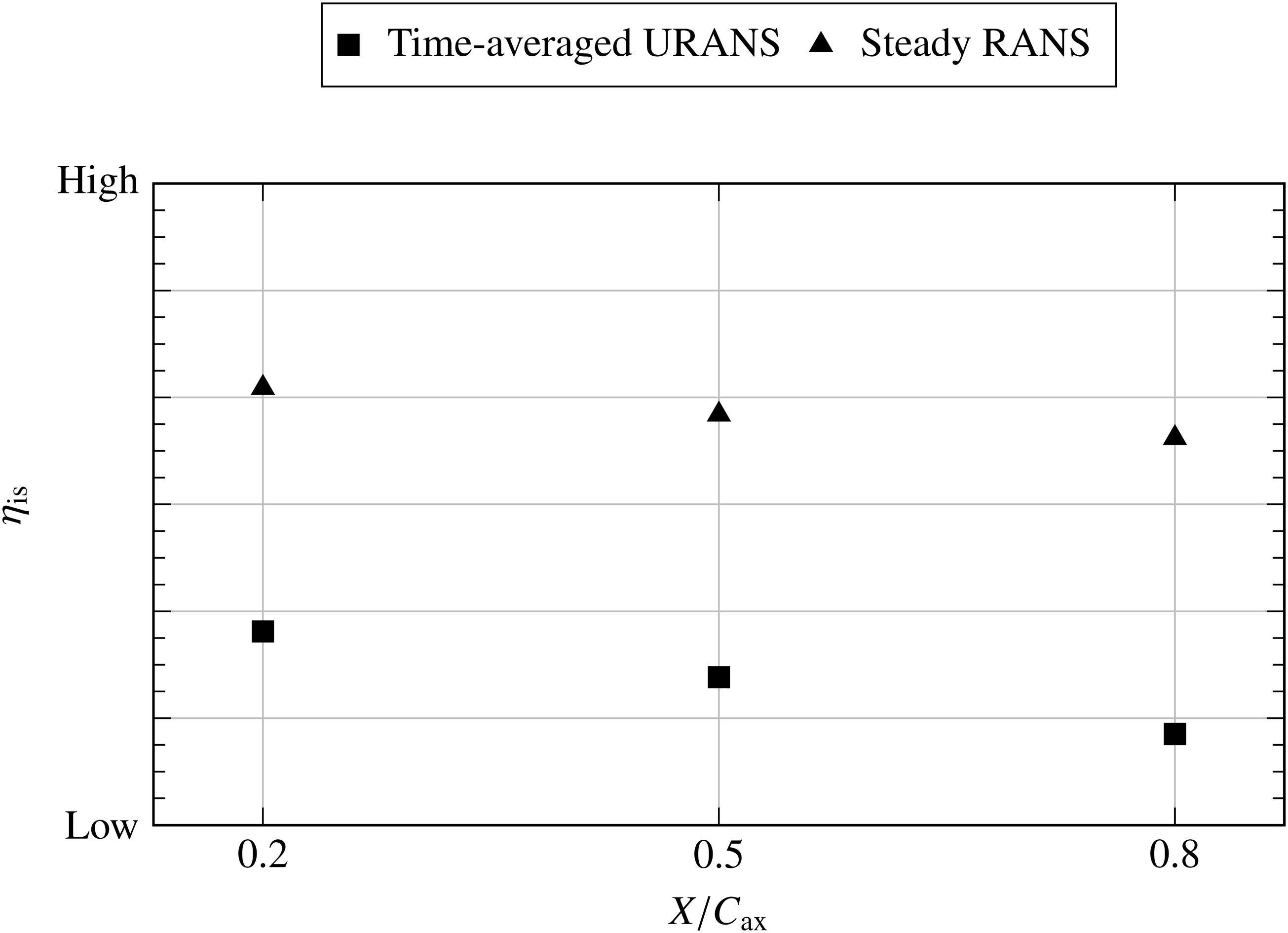
The resulting system efficiency is depicted in Figure 8. In addition to the URANS simulations, results from steady-state calculations are also considered. Despite steady-state CFD not capturing stator-rotor interaction, the overall trend does agree: The smallest gap investigated represents the optimum configuration.
Conclusions
The effect of the axial-gap size on system losses is quantified using a functional separation of different entropy sources, such as end-wall friction, profile loss, and secondary flow. For these individual terms, different trends with regard to axial-gap variation can be identified. For the quasi two-dimensional flow field in the mid-span region, larger axial gaps are beneficial due to the reduced wake dilation and associated mixing losses in the downstream row. For the smallest gap, unsteady wake-blade interaction is a major source of two-dimensional loss. A more extensive investigation of the flow region outside of the boundary layers revealed, however, that a clear distinction into two- and three-dimensional flow is valid only for a very small flow region at the mid-span. All other flow regions are afflicted by a strong interaction between – or even merging of – various phenomena, which are not just a superposition of multiple effects. In contrast to the trend immediately at the mid-span, end-wall regions show an increase in losses for larger axial gaps, due to higher friction and stronger secondary flow. End-wall related losses contribute almost 2/3 of the entire system loss: It is found to be the dominant loss contribution.
The optimal axial gap is, therefore, an ideal compromise between individual loss contributions for a given turbine configuration. For the configurations investigated, the optimal gap equals 20% of the stator axial chord length.
Based on the framework derived in the present work, the interdependency of the axial-gap size effect and secondary design parameters will be the subject of further research. It is, for example, self-evident that a higher aspect ratio would lead to profile losses becoming a more dominant factor, which would then shift the optimal gap towards a larger size. Nevertheless, a more refined distinction criterion between end-wall boundary-layer and wake flow should be derived before proceeding further.
Since the focus of this paper was the time-averaged flow field, instantaneous unsteady effects were generally neglected. Unsteady losses, therefore, remain a factor to be considered in greater detail.